Meteorological constraints on oceanic halocarbons above the Peruvian upwelling

(1)

www.atmos-chem-phys.net/16/12205/2016/

doi:10.5194/acp-16-12205-2016

Meteorological constraints on oceanic halocarbons above the Peruvian upwelling

Steffen Fuhlbrügge¹, Birgit Quack¹, Elliot Atlas², Alina Fiehn¹, Helmke Hepach¹, and Kirstin Krüger³

1GEOMAR Helmholtz Centre for Ocean Research Kiel, Kiel, Germany

2Rosenstiel School for Marine and Atmospheric Sciences, Miami, Florida, USA

3Department of Geosciences, University of Oslo, Oslo, Norway Correspondence to:Kirstin Krüger (kirstin.krueger@geo.uio.no)

Received: 23 June 2015 – Published in Atmos. Chem. Phys. Discuss.: 31 July 2015 Revised: 29 August 2016 – Accepted: 30 August 2016 – Published: 29 September 2016

Abstract. During a cruise of R/V METEOR in Decem- ber 2012 the oceanic sources and emissions of various halogenated trace gases and their mixing ratios in the marine atmospheric boundary layer (MABL) were investigated above the Peruvian upwelling. This study presents novel observations of the three very short lived substances (VSLSs) – bromoform, dibromomethane and methyl iodide – together with high-resolution meteorological measurements, Lagrangian transport and source–loss calculations. Oceanic emissions of bromoform and dibromomethane were relatively low compared to other upwelling regions, while those for methyl iodide were very high. Radiosonde launches during the cruise revealed a low, stable MABL and a distinct trade inversion above acting as strong barriers for convection and vertical transport of trace gases in this region. Observed atmospheric VSLS abundances, sea surface temperature, relative humidity and MABL height correlated well during the cruise. We used a simple source–loss estimate to quantify the contribution of oceanic emissions along the cruise track to the observed atmospheric concentrations. This analysis showed that averaged, instantaneous emissions could not support the observed atmospheric mixing ratios of VSLSs and that the marine background abundances below the trade inversion were significantly influenced by advection of regional sources. Adding to this background, the observed maximum emissions of halocarbons in the coastal upwelling could explain the high atmospheric VSLS concentrations in combination with their accumulation under the distinct MABL and trade inversions. Stronger emissions along the nearshore coastline likely added to the elevated abundances under the steady atmospheric conditions. This study underscores the

importance of oceanic upwelling and trade wind systems on the atmospheric distribution of marine VSLS emissions.

1 Introduction

Oceanic fluxes of short-lived halocarbons contribute to reactive halogens in the atmosphere, where they are subsequently involved in ozone chemistry, aerosol formation, and other chemical cycles that influence the fate of pollutants and climate (McGivern et al., 2000; Saiz-Lopez and von Glasow, 2012; Simpson et al., 2015). Recent studies have identified open-ocean upwelling areas in the Atlantic as large source regions for a number of brominated and iodinated oceanic trace gases (Quack et al., 2004, 2007; O’Brien et al., 2009;

Raimund et al., 2011; Hepach et al., 2015). Their sources are related to biological and chemical processes in the productive waters of the upwelling. Although oceanic upwelling and nearshore regions are small compared to the global ocean area, they are known to significantly contribute to the oceanic bromocarbon fluxes (Quack and Wallace, 2003; Butler et al., 2007; Ziska et al., 2013). In the upwelling regions the compounds are emitted from the ocean and are horizontally transported and vertically mixed in the marine atmospheric boundary layer (MABL) (Carpenter et al., 2010). Meteoro- logical conditions strongly influenced the atmospheric mixing ratio of the marine compounds bromoform (CHBr₃), dibromomethane (CH₂Br₂) and also methyl iodide (CH₃I) (e.g. Fuhlbrügge et al., 2013; Hepach et al., 2014). The combination of a pronounced low MABL above cold upwelling waters with high concentrations and emissions of the com-

(2)

pounds causes elevated atmospheric mixing ratios. In a negative feedback process, these high atmospheric mixing ratios reduce the marine emissions through a decrease in the sea–

air concentration gradient (Fuhlbrügge et al., 2013). Similar relationships would be expected for other oceanic upwelling areas, where not only the oceanic emissions but also meteorological conditions in the lowermost atmosphere, i.e. the height, type and structure of the boundary layer and trade inversion, determine the very short lived substance (VSLS) abundance and atmospheric distribution. The intense oceanic upwelling in the south-eastern Pacific off the coast of Peru transports large amounts of subsurface water to the ocean surface and creates one of the most productive oceanic regions worldwide (Codispoti et al., 1982). We therefore ex- pect elevated levels of short-lived halocarbons in the Pe- ruvian upwelling zone as a potential source for the atmosphere. Indeed, Schönhardt et al. (2008) detected elevated IO columns during September and November 2005 along the Peruvian coast with the SCIAMACHY satellite instrument and inferred elevated iodine source gases from the Peruvian upwelling.

Although recent studies have investigated halocarbons in the eastern Pacific (Yokouchi et al., 2008; Mahajan et al., 2012; Saiz-Lopez et al., 2012; Gómez Martin et al., 2013;

Liu et al., 2013), few have concentrated on the Peruvian upwelling in the south-eastern Pacific. Only measurements of methyl iodide exist in this region, revealing atmospheric abundances of 7 ppt (Rasmussen et al., 1982). Observations of bromocarbons above the Peruvian upwelling are currently lacking.

In this study we present a novel dataset of meteorological parameters, oceanic concentrations and atmospheric abundances of VSLSs and calculated emissions along the Peru- vian coast and in the upwelling. The goal of this study is to assess the influence of oceanic upwelling and meteorological conditions on the atmospheric VSLS abundances above the Peruvian upwelling, and to determine the contribution of the local oceanic emissions to MABL and free-tropospheric VSLS concentrations.

2 Data and methods

The Cruise M91 on R/V METEOR from 1 to 26 Decem- ber 2012 started and ended in Lima, Peru (Fig. 1a). The ship reached the northernmost position during the cruise on 3 December 2012 at 5^◦S. In the following 3 weeks the ship headed southward and reached its southernmost position at 16^◦S on 21 December 2012. During this time the track alter- nated between open-ocean sections and sections close to the Peruvian coast (up to 10 km distance) in the cold upwelling waters. A focus on diurnal variations was accomplished by 24 h sampling at six stations along the cruise track.

2.1 Meteorological observations

Meteorological observations of surface air temperature (SAT), sea surface temperature (SST), relative humidity, air pressure, wind speed and direction were taken every second at about 25 m height above sea level on R/VMETEOR and averaged to 10 min intervals for our investigations. At- mospheric profiles of temperature, wind, and humidity were obtained by 98 radiosonde launches (00:00, 06:00, 12:00, 18:00 UTC) and additionally at 3 h intervals during the diurnal stations along the cruise track, using Vaisala RS92 radiosondes. Due to permission limitations, radiosondes could not be launched within 12 nmi of the Peruvian coast. The collected radiosonde data were integrated in near-real time into the Global Telecommunication System (GTS) to improve operational weather forecast models and meteorological reanalysis for this region, which were used as input parameters for our trajectory calculations.

2.2 MABL

The radiosonde data are used to identify the height of the MABL, which is the atmospheric surface layer above the ocean in which trace gas emissions are mixed on a short timescale of an hour or less by convection and turbulence (Stull, 1988). Two different kinds of MABL can be distin- guished that are characterized by the gradient of the virtual potential temperatureθv. A negative or neutral gradient reveals an unstable convective layer, while a positive gradient reveals astableatmospheric layer. In the case of an increase in the virtual potential temperature (positive gradient) near the surface, mixing in the MABL is suppressed.

The upper limit of the convective MABL is set by a stable layer, e.g. a temperature inversion or a significant reduction in air moisture, and is typically found above open-ocean regions between 100 m and 3 km height (Stull, 1988; Seibert et al., 2000). For determining the height of this stable layer above the convective MABL, we use the practical approach described in Seibert et al. (2000) and compute the virtual potential temperature for which an increase with altitude indicates the base of a stable layer. In this study, its base is increased by half of its thickness, which is the definition for the MABL height. Over oceanic upwelling regions the stable layer can even descend to the ocean surface (e.g. Höflich et al., 1972; Fuhlbrügge et al., 2013).

Estimates for atmospheric surface stability and MABL conditions can be also obtained from variations in the surface humidity. While the absolute humidity determines the amount of water in a specific volume of air, the relative humidity is the ratio of the partial pressure of water vapour to the equilibrium vapour pressure at the observed temperature.

Variations in the SAT directly influence the relative humidity at the surface (Sect. 3.1). Elevated relative humidity in this oceanic region likely points to stable layers with suppressed mixing of surface air and to a low and stable MABL

(3)

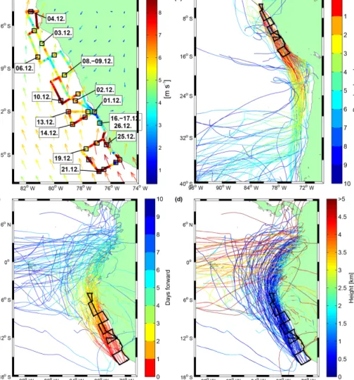
Figure 1. (a)10 min mean of wind speed observed on R/VMETEORdisplayed along the cruise track; monthly mean (December 2012) of 10 m wind speed and direction from ERA-Interim displayed as arrows.(b)Extract from 10-day FLEXPART back-trajectories coloured according to the time until they reach the specific ship position on the cruise track of R/VMETEOR (black).(c)Extract from 10-day FLEXPART forward trajectories coloured according to the time since they were released. (d)Same as(c)but coloured according to the height (km) of the trajectories.

height. Relative humidity is also used to derive the MABL height above the upwelling areas close to the coast, where radiosonde launches were not permitted (Sect. 2.1). We applied a multiple linear regression (Eq. 1), using meteorological parameters along the cruise track that had significant correlations (see Sect. 3.5) with the observed MABL height (relative humidity (x1), SAT (x2), SST (x3)and wind speed (x4)):

MABL height=b1x1+b2x2+b3x3+b4x4, (1) with b1= −0.0117, b2=0.0202, b3=0.0467, and b4= 0.0089.

Missing MABL data close to the coast were then com- pleted with the regressed MABL height (Eq. 1) at the VSLS sampling location.

2.3 Atmospheric and oceanic VSLS measurements and sea–air fluxes

A total of 198 air samples was collected at 3-hourly intervals during the cruise at about 20 m height above sea level on the fifth superstructure deck of R/VMETEORusing a port- side jib of 5–6 m. The air samples were pressurized to 2 atm in pre-cleaned stainless steel canisters with a metal bellows pump and were analysed at the Rosenstiel School for Ma- rine and Atmospheric Sciences (RSMAS, Miami, Florida) within 6 months after the cruise. Details about the analysis, the instrumental precision and the preparation of the samples are described in Schauffler et al. (1999) and Fuhlbrügge et al. (2013). The VSLS atmospheric mixing ratios were calculated with a NOAA standard (SX3573) from GEOMAR.

Starting from 9 December 2012, 102 water samples were taken at 3 h intervals at a depth of 6.8 m from a continuously

(4)

working water pump in the hydrographic shaft, an opening in the base of the hull of R/VMETEOR. The samples were then analysed for bromoform, dibromomethane, methyl iodide and other halogenated trace gases by a purge and trap system attached to a gas chromatograph combined with an ECD (electron capture detector). The analysis has a precision of 10 % (1σ) determined from duplicate samples. The approach is described in detail by Hepach et al. (2014).

The sea–air flux (F )of bromoform, dibromomethane and methyl iodide is calculated with k_w as a transfer coefficient and1c as a concentration gradient between the water and equilibrium water concentration determined from the atmospheric concentrations (Eq. 2). The transfer coefficient was determined by the air–sea gas exchange parameterization of Nightingale et al. (2000) after a Schmidt number (Sc) correction for the three gases (Eq. 3).

F =kw·1c (2)

kw=kCO₂·Sc⁻¹²

600 (3)

Details on deriving the air–sea concentration gradient and emissions are further described in Hepach et al. (2014) and references therein.

2.4 Trajectory calculations

The Lagrangian particle dispersion model FLEXPART of the Norwegian Institute for Air Research in the Department of Atmospheric and Climate Research (Stohl et al., 2005) was used for trajectory calculations to analyse the air mass origins and the transport of surface air masses along the cruise track to the free troposphere (Stohl et al., 1998; Stohl and Trickl, 1999). The model includes moist convection and turbulence parameterizations in the atmospheric boundary layer and free troposphere (Stohl and Thomson, 1999; Forster et al., 2007).

We use the ECMWF (European Centre for Medium-Range Weather Forecasts) reanalysis product ERA-Interim (Dee et al., 2011) with a horizontal resolution of 1^◦×1^◦and 60 vertical model levels as meteorological input fields, providing air temperature, horizontal and vertical winds, boundary layer height, specific humidity, and convective and large-scale pre- cipitation with a 6-hourly temporal resolution. Trajectories were released every 3 to 6 h coincident with VSLS measurements along the cruise track on R/V METEOR. At each of these release points 10 000 forward- and 50 back-trajectories with a total runtime of ∼30 days were initiated from the ocean surface within ±30 min and ∼20 m distance of the measurements. In total 98 release points for the forward- and back-trajectory calculations were analysed, determined by the spatial resolution of ERA-Interim data along the Peru- vian coast, defining the land–sea mask of our trajectory calculations.

2.5 Oceanic contribution to MABL VSLS abundances To estimate the contribution of local oceanic sources to the atmospheric mixing ratios in the lowermost atmosphere above the Peruvian upwelling, we apply a mass balance concept to the oceanic emissions, the timescales of air mass transport and the chemical loss (Fuhlbrügge et al., 2016).

First we define a box above each release event with a size of∼400 m²around the measurement location and the height of the MABL and assume steady state in the box (Fig. 2).

During each trajectory release event we assume the specific sea–air flux to be constant and the emissions to be homogeneously mixed within the box. Then the contribution of the sea–air flux is computed as the ratio of the VSLS flux from the ocean into the MABL (in moles per day) and the total amount of VSLSs in the box (in moles). This ratio is defined as the oceanic delivery (OD) and is given in percentage per day. In addition to the delivery of oceanic VSLSs to the box, the loss of VSLSs out of the box and into the free troposphere is defined as the convective loss (COL) and this quantity is derived from the mean residence time of the FLEXPART trajectories in the box during each release event. Note that the COL indicates the loss of surface air due to all kinds of vertical movement out of the box. Since this is a loss process, COL is given as a negative quantity expressed as percentage per day. The chemical degradation of VSLSs by OH and photolysis in the MABL is calculated from the chemical lifetime of each compound in the MABL. We use lifetimes of 15 days for bromoform, 94 days for dibromomethane and 4 days for methyl iodide (Carpenter et al., 2014), representative of the tropical boundary layer. The chemical loss (CL) is given as a negative quantity in percentage per day. OD, COL and CL must be balanced by an advective transport of air masses in and out of the box. The change of the VSLSs through advective transport is defined as advective delivery (AD) and is also given in percentage per day.

To estimate the relative importance of ocean emissions (OD) to the halocarbon loss through vertical mixing (COL) we define an oceanic delivery ratio (ODR) (Eq. 4) as the ratio between OD and COL:

ODR= OD[% d⁻¹] COL[% d⁻¹]

=sea–air flux contribution[% d⁻¹]

loss of box air to the FT[% d⁻¹]. (4) Similarly, the chemical loss in the box (CL) and the change in VSLSs due to advection (AD) are related to COL to get the chemical loss ratio (CLR) and the advective delivery ratio (ADR). From mass balance considerations, ODR – CLR+ADR=1. Since CL, OD and AD are divided by COL, ratios for source processes are positive and negative for loss processes (Fuhlbrügge et al., 2016).

(5)

Figure 2. Schematic summary of the components of the applied mass-balance concept from Fuhlbrügge et al. (2016): oceanic delivery (OD), the convective loss (COL), the chemical loss (CL), the advective delivery (AD), the oceanic delivery ratio (ODR), the chemical loss ratio (CLR) and the advective delivery ratio (ADR). The shaded area reflects an area of 400 m².

3 Observations on R/VMETEOR 3.1 Meteorology

The Peruvian coast is dominated by the Southern Hemi- sphere trade wind regime with predominantly south-easterly winds (Fig. 1). The Andes, which are known to act as a barrier to zonal wind in this region, affect the horizontal air mass transport along the coast (Fig. 1b–d). The steeply sloping mountains at the coast form strong winds paral- lel to the South American coastline (Garreaud and Munoz, 2005). The 10-day back-trajectories reveal a mix of open- ocean and coastal air masses (Fig. 1). The average wind direction observed on R/V METEOR during the cruise is 160^◦±34^◦(mean±σ )with a moderate average wind speed of 6.2±2.2 m s⁻¹ (Fig. 3b). ERA-Interim reveals similar winds along the cruise track with a mean wind speed of 5.6±1.8 m s⁻¹ and a mean wind direction of 168^◦±21^◦ (not shown here). The divergence of the wind-driven Ek- man transport along the Peruvian coast leads to the observed oceanic upwelling of cold waters. The most intense upwelling was observed several times near the coast, where both SST and SAT rapidly drop from 19–22^◦C to less than 18^◦C (Fig. 3a). The impact of the cold upwelling water on the air masses is also visible in the observed humidity fields (Fig. 3c). Here, the decreasing SAT reduces the amount of water vapour that the surface air is able to contain, leading to an increase in the relative humidity and indicating a stable atmospheric surface layer with suppressed vertical mixing. The absolute humidity stays constant or even decreases above the oceanic upwelling due to condensation of water vapour when surface air cools and becomes saturated, coinciding with fog observations on the ship. A decrease in the absolute humid-

SAT [oC]

(a)

14 16 18 20 22 24

SST [oC]

14 16 18 20 22 24

Rel. hum. [%]

(c)

70 75 80 85 90 95 100

Abs. hum. [g m−3]

12 13 14 15 16 17 18

Wind dir.

(b)

N E S W N

Wind spd. [m s ]

0 5 10 15 20

CHBr3 [ppt]

(e)

0 1 2 3 4 5 6

CH2Br2, CH3I [ppt]

0.5 1 1.5 2 2.5 3 3.5

CH2Br2 / CHBr3 (f)

0.3 0.4 0.5 0.6 0.7 0.8

CHBr3 [nmol m−2h−1]

(g)

−1 0 1 2 3 4 5

CH2Br2, CH3I [nmol m−2h−1]

Date [UTC 2012]

01. Dec 05. Dec 09. Dec 13. Dec 17. Dec 21. Dec 25. Dec−1 0 1 2 3 4 5 CHBr3 [pmol L−1]

(d)

0 10 20 30 40

CH2Br2, CH3I [pmol L−1]

0 10 20 30 40

−1

Figure 3.Observations during 1–25 December 2012 on R/VME- TEOR. Diurnal stations are indicated by grey background shading.

(a)10 min mean of the SAT (orange) and the SST (blue) in^◦C. Ac- cording to SST decrease, upwelling regions are marked with light- blue background shading in(b–e).(b)10 min mean of wind direction in cardinal directions (ochre) and wind speed in m s⁻¹(blue).

(c)10 min mean of relative humidity in % (dark blue) and absolute humidity in gm⁻³ (green).(d)Oceanic surface concentrations of bromoform (CHBr₃, blue), dibromomethane (CH₂Br₂, dark grey) and methyl iodide (CH₃I, red) in pmol L⁻¹.(e)Atmospheric mixing ratios of bromoform, dibromomethane and methyl iodide in ppt.

(f)Concentration ratio of atmospheric dibromomethane and bromoform.(g)Sea–air flux for bromoform, dibromomethane and methyl iodide in nmol m⁻²h⁻¹.

ity outside the upwelling points to a change in advected air masses (e.g. 9, 11, 19 December 2012; Fig. 3c).

3.2 VSLS abundances and oceanic emissions

Surface water samples of the coastal upwelling areas show elevated VSLS concentrations compared to the open ocean

(6)

Table 1.Oceanic concentrations, atmospheric mixing ratios and sea–air fluxes of bromoform (CHBr₃), dibromomethane (CH₂Br₂), the concentration ratio of bromoform and dibromomethane and methyl iodide (CH₃I) observed during the cruise. Values are given in mean±1σ. The range is given in square brackets.

CHBr₃ CH₂Br₂ CH₂Br₂/CHBr₃ CH₃I Oceanic concentration 6.6±5.5 4.3±3.4 0.9±0.8 9.8±6.3

(pmol L⁻¹) [0.2–21.5] [0.2–12.7] [0.1–4.2] [1.1–35.4]

Atmospheric mixing ratio 2.9±0.7 1.3±0.3 0.4±0.1 1.5±0.5

(ppt) [1.5–5.9] [0.8–2.0] [0.3–0.7] [0.6–3.2]

Sea–air flux 117±492 245±299 0.4±8.6 856±623

(pmol m⁻²h⁻¹) [−477–1916] [−112–1169] [−24.5–48.9] [18–4179]

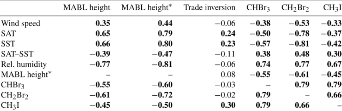
Table 2. Spearman correlation coefficients (R) of meteorological parameters, MABL height and trade inversion height correlated with atmospheric bromoform (CHBr₃), dibromomethane (CH₂Br₂)and methyl iodide (CH₃I). MABL height^∗is the determined MABL height from the radiosonde launches, complemented by the regressed MABL height (Sect. 3.3). Bold coefficients are significant with apvalue of

<0.05.

MABL height MABL height^∗ Trade inversion CHBr₃ CH₂Br₂ CH₃I

Wind speed 0.35 0.44 −0.06 −0.38 −0.53 −0.33

SAT 0.65 0.79 0.24 −0.50 −0.78 −0.37

SST 0.66 0.80 0.23 −0.57 −0.81 −0.42

SAT–SST −0.39 −0.47 −0.11 0.38 0.48 0.30

Rel. humidity −0.77 −0.81 −0.06 0.74 0.77 0.67

MABL height^∗ – – 0.08 −0.55 −0.61 −0.45

CHBr₃ −0.55 −0.60 −0.03 – 0.79 0.79

CH₂Br₂ −0.61 −0.72 −0.02 0.79 – 0.66

CH₃I −0.45 −0.50 0.30 0.79 0.66 –

for all compounds, especially for methyl iodide (Hepach et al., 2016). Atmospheric mixing ratios of bromoform were on average 2.91±0.68 ppt (Table 1). Dibromomethane mixing ratios (average 1.25±0.26 ppt) show a similar pattern and good correlation with bromoform (Table 2). Elevated mixing ratios for all three compounds are generally found above the intense cold oceanic upwelling regions close to the Peruvian coast (Fig. 3e). While the bromocarbons double above the upwelling, methyl iodide mixing ratios increase up to 5-fold, demonstrating its stronger accumulation in the low and stable boundary layer.

The concentration ratio of atmospheric dibromomethane to bromoform can be used as an indicator of bromocarbon sources along coastal areas. Low ratios of about 0.1 have been observed in coastal source regions and have been in- terpreted as the emission ratios of macro algae (Yokouchi et al., 2005; Carpenter et al., 2003). The shorter chemical lifetime of bromoform (15 days) in contrast to dibromomethane (94 days) in the boundary layer leads to an increase in the ratio during transport as long as the air mass is not newly enriched with bromoform (Carpenter et al., 2014). This concentration ratio generally decreased from the north to the south (Fig. 3f), implying an intensification of fresh bromoform sources towards the southern part of the cruise track,

which is also reflected by increasing water concentrations.

Atmospheric methyl iodide measurements along the cruise track reveal a mean mixing ratio of 1.54±0.49 ppt, which, similar to the two bromocarbons, maximizes over the coastal upwelling regions (Fig. 3e).

Oceanic emissions during the cruise were calculated from the approximately synchronous measurements of sea water concentrations and atmospheric mixing ratios, sea surface temperatures and wind speeds, measured on R/V METEOR. Oceanic concentrations and atmospheric mixing ratios of each compound were weakly or not at all correlated (Rbromoform=0.00,Rdibromomethane=0.29 and Rmethyl iodide=0.34). Mean sea–air fluxes of the bromocarbons during the cruise are low, at 117±492 pmol m⁻²h⁻¹ for bromoform and 245±299 pmol m⁻² h⁻¹ for dibromomethane compared to other oceanic regions (e.g.

Fuhlbrügge et al., 2013; Hepach et al., 2015), but for methyl iodide the fluxes were elevated at 856±623 pmol m⁻²h⁻¹ (Fig. 3g, Table 1). Further investigations of the distributions and sources of iodinated compounds during this cruise are carried out by Hepach et al. (2016).

(7)

Figure 4. (a–c)Radiosonde observations of the lower 6 km of the atmosphere between 2 and 24 December 2012 on R/VMETEOR.

Shown are(a)the relative humidity in %,(b)the meridional wind in m s⁻¹and(c)the gradient of the virtual potential temperature in 10⁻²K m⁻¹in combination with the determined MABL height (black) and the associated MABL height above the oceanic upwelling from the multiple linear regressions (blue).(d)Distribution of 10-day FLEXPART forward trajectories. The black contour lines give the amount of trajectories in percentage reaching an altitude of 0–6 km height within the 10 days. The elapsed time in days until these trajectories reach this height is reflected by the colour shading.

The white line shows the ERA-Interim MABL height at the ship’s position. Trajectory analyses gaps close to the coast are whitened (Sect. 2.4). Theyaxes are non-linear.

3.3 Lower atmosphere conditions

A strong positive vertical gradient of relative humidity at

∼1 km height (Fig. 4a) indicates an increase in the atmospheric stability. This convective barrier, known as the trade inversion (Riehl, 1954, 1979; Höflich, 1972), is also reflected in the meridional wind (Fig. 4b). Below∼1 km altitude the south-easterly trade winds create a strong positive meridional wind component, also visible in the forward trajecto-

ries (Fig. 1c–d). The flow of air masses in the Hadley cell back to the subtropics causes a predominantly northerly wind above ∼1 km height. The intense increase in θv in combination with the relative humidity decrease and the wind shear at∼1 km height identifies this level as a strong vertical transport barrier (Fig. 4c). Above the cold upwelling water, temperature inversions create additional stable layers above the surface, leading to very low MABL heights of<100 m (e.g. on 3, 8 or 17 December 2012) and a reduced vertical transport of surface air. The mean MABL height from the radiosonde observations is 370±170 m (ERA-Interim 376±169 m). The relative humidity, SAT, SST and wind speed show significant correlations with the observed MABL height (Table 2). The regressed MABL heights (Sect. 2.2) show a distinct decrease above the cold upwelling regions close to the coast with 158±79 m on average. Taking the regressed MABL height into account, the mean MABL height during the cruise decreases to 307±177 m. The stable atmospheric conditions from the surface to the trade inversion lead to strong transport barriers also visible in the accumulation of below 2-day-old air masses within the first kilometre of the atmosphere (Fig. 4d).

3.4 Contribution of oceanic emissions to VSLS abundances in the MABL

We estimate the contribution of oceanic emissions to mixing ratios within the MABL and below the trade inversion with a VSLS source–loss estimate (Table 3). The mean loss of VSLSs out of the MABL box is 351.0 % d⁻¹and equal for all compounds, since it is computed from the loss of trajectories out of the box. The loss is based on a mean residence time of the FLEXPART trajectories of 7 h in the observed in situ MABL height during the cruise. The ratio of the indi- vidual OD of each compound and the COL at this location results in the particular ODR for each compound. The ODR reveals that on average only 3 % of the observed atmospheric bromoform in the MABL originates from local oceanic emissions and 99 % are advected including a chemical loss of 2 %.

The numbers show that the observed mean atmospheric concentrations cannot be explained by the mean local oceanic emissions. While the surface air masses can leave the MABL within hours, they are restricted from entering the free troposphere through the trade inversion. FLEXPART trajectories indicate an average residence time of air 48 h below the average trade inversion height of 1.1 km. During the 48 h and the prevailing southerly mean wind speed of 6.2 m s⁻¹oceanic VSLS emissions can accumulate over a fetch of 10^◦latitude.

The impact of these conditions on VSLS emissions is discussed in Sect. 4.

(8)

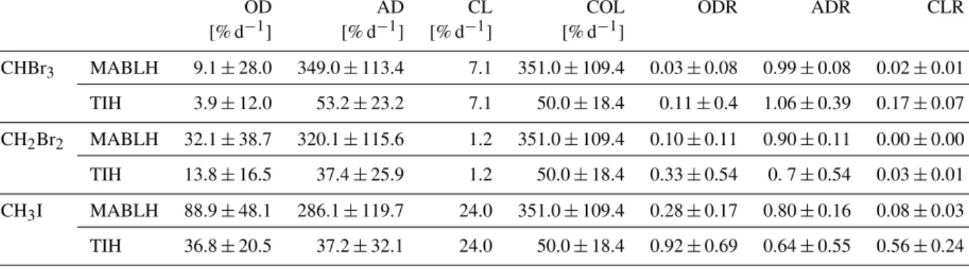
Table 3.VSLS source–loss calculations: mean±1σ of oceanic delivery (OD), advective delivery (AD), chemical loss (CL), convective loss (COL), oceanic delivery ratio (ODR), advective delivery ratio (ADR) and chemical loss ratio (CLR) of bromoform (CHBr₃), dibromomethane (CH₂Br₂)and methyl iodide (CH₃I). Parameters have been computed for a box with the vertical extension of the in situ MABL height (MABLH) and a mean trade inversion height (TIH) of 1.1 km.

OD AD CL COL ODR ADR CLR

[% d⁻¹] [% d⁻¹] [% d⁻¹] [% d⁻¹]

CHBr₃ MABLH 9.1±28.0 349.0±113.4 7.1 351.0±109.4 0.03±0.08 0.99±0.08 0.02±0.01 TIH 3.9±12.0 53.2±23.2 7.1 50.0±18.4 0.11±0.4 1.06±0.39 0.17±0.07 CH₂Br₂ MABLH 32.1±38.7 320.1±115.6 1.2 351.0±109.4 0.10±0.11 0.90±0.11 0.00±0.00 TIH 13.8±16.5 37.4±25.9 1.2 50.0±18.4 0.33±0.54 0. 7±0.54 0.03±0.01 CH₃I MABLH 88.9±48.1 286.1±119.7 24.0 351.0±109.4 0.28±0.17 0.80±0.16 0.08±0.03 TIH 36.8±20.5 37.2±32.1 24.0 50.0±18.4 0.92±0.69 0.64±0.55 0.56±0.24

3.5 Meteorological constraints on atmospheric VSLSs in the MABL

We find significantly high correlations between meteorological parameters and the abundances of bromoform, dibromomethane and methyl iodide (Table 2) along the Peruvian coast. The predominantly moderate winds during the cruise are negatively correlated with the atmospheric VSLSs and positively correlated with the MABL height. This shows that VSLS abundances tend to be elevated during periods of lower wind speeds, which lead to reduced mixing of surface air and therefore to lower MABL heights, in particular above the coastal upwelling events on 11, 15–17 and 24 Decem- ber 2012. No significant correlation is found between the oceanic emissions and the atmospheric VSLSs (not shown), revealing a stronger influence of the wind speed on the atmospheric accumulation of the VSLSs rather than the oceanic emissions. SAT and SST are both negatively correlated with atmospheric VSLSs, since elevated atmospheric VSLS mixing ratios are generally found close to the oceanic upwelling regions with low SATs and SSTs. In these regions the decrease in the SATs leads to an increase in the relative humidity (Sect. 3.1), which results in a significantly high correlation with the VSLSs. Since SAT and SST impact the MABL, which affects the relative humidity, these correlation coefficients are co-correlated. Correlation coefficients between the MABL height and the VSLSs are slightly lower (Table 2). A principal component analysis of the parameters in Table 2 also confirmed the strong connection between SAT, SST, MABL height, relative humidity and atmospheric mixing ratios of bromoform and dibromomethane (not shown here).

3.6 Comparison to other oceanic regions

Surface water concentrations of bromoform in the Peruvian upwelling during the cruise were generally lower compared to observations in other coastal upwelling regions, e.g. the Mauritanian upwelling (Carpenter et al., 2010; Fuhlbrügge

et al., 2013; Hepach et al., 2014). While dibromomethane concentrations are comparable, methyl iodide concentrations are almost 8 times higher than in the Mauritanian upwelling (Fig. 3d, Table 1; Hepach et al., 2014). Atmospheric mixing ratios of bromoform and dibromomethane are significantly lower above the Peruvian upwelling compared to observations above the Mauritanian upwelling, while methyl iodide mixing ratios are comparable (Fuhlbrügge et al., 2013).

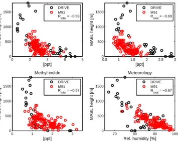
MABL properties (height and stability) reveal a stronger influence on the VSLS abundances at the marine surface during the DRIVE cruise covering the Mauritanian upwelling compared to this study (M91) covering the Peruvian upwelling (Fig. 5). Observed local oceanic bromocarbon emissions can only partly explain the atmospheric VSLS concentrations above the Peruvian upwelling, while above the Mauritanian upwelling the generally higher emissions could occasionally explain up to 100 % of the atmospheric abundances of VSLSs in very low and stable MABL conditions (Fuhlbrügge et al., 2013; Hepach et al., 2014). The predominantly southerly winds along the western coastline of Peru allowed only minor continental influence on the offshore coastal atmosphere, while the Mauritanian upwelling showed a larger variation in maritime and continental air masses. Al- though our investigations revealed low MABL heights close to the Peruvian coast, the maritime air mass origin led to less developed surface inversions compared to those observed above the Mauritanian upwelling, where the higher emissions led to a stronger and more variable enrichment in the MABL. This can lead to the observed higher correlation coefficients between the MABL height and the VSLS abundances in the Mauritanian upwelling (Fig. 5).

Compared to the two eastern boundary upwelling systems, observed VSLS sources at the coasts of the South China and Sulu seas were significantly higher (Fuhlbrügge et al., 2016). Despite the elevated emissions there, the atmospheric VSLS abundances in the West Pacific were lower, due to the presence of a convective active, well-ventilated MABL. The

(9)

0 2 4 6 8 0

500 1000 1500

Bromoform

[ppt]

MABL height [m]

DRIVE M91 R_total = −0.69

0.5 1 1.5 2 2.5 3

0 500 1000 1500

Dibromomethane

[ppt]

MABL height [m]

0 1 2 3

0 500 1000 1500

Methyl iodide

[ppt]

MABL height [m]

70 80 90 100

0 500 1000 1500

Meteorology

Rel. humidity [%]

MABL height [m]

Figure 5.Scatter plots of near-surface atmospheric mixing ratios of bromoform, dibromomethane, methyl iodide and relative humidity vs. MABL height. Black circles reflect observations from the DRIVE campaign covering the Mauritanian upwelling (Fuhlbrügge et al., 2013) and red circles from this study (M91) covering the Pe- ruvian upwelling.R_totalgives the Spearman correlation coefficients for both datasets together.

comparison between the different regions demonstrates that the atmospheric abundances of VSLSs over the ocean are significantly controlled by prevailing meteorological conditions next to their oceanic sources and emissions.

4 Discussion

Compounds emitted from the Peruvian upwelling are first homogeneously distributed within the MABL in only a few hours according to the observations during the M91 cruise.

Afterwards the emitted compounds are distributed within and transported below the trade inversion. For air masses above or close to oceanic upwelling regions, the MABL height is the first transport barrier on short timescales, while the trade inversion acts as a second, more pronounced barrier for vertical transport on longer timescales. The residence time of air masses below the trade inversion of 48 h leads to a stronger enrichment of VSLSs from the oceanic emissions, reflected in the OD (Table 3), compared to the enrichment in the MABL. For the mean wind speed of 6.2 m s⁻¹and wind direction of 160^◦observed during the cruise, air masses accumulate oceanic emissions from approximately 1.5^◦latitude distance during the residence time of 7 h in the MABL and below the trade wind inversion from approximately 10^◦latitude during 48 h, which covers the southern Peruvian as well as part of the Chilean coast.

4.1 Accumulation of background concentrations The observed near-surface atmospheric mixing ratios suggest background concentrations of the compounds which were around 2 ppt for CHBr₃, 0.8 ppt of CH₂Br₂ and 1 ppt for CH₃I (Figs. 3e and 5). The back-trajectories revealed air masses originating from the southern Peruvian and Chilean coast, which were transported along the coast for about 5 days. In combination with a stable MABL and a distinct trade inversion acting as strong barriers to the vertical mixing of trace gases, these air masses travelled close to the surface where they could be enriched during 48 h with regional emissions before they enter the free troposphere. Mean emissions of around 2000 pmol m⁻²h⁻¹for CHBr₃and for CH₃I and 800 pmol m⁻²h⁻¹for CH₂Br₂would have been needed during the residence time of 48 h of air below the trade wind inversion to reach the elevated background concentrations observed on board the ship. These emissions are close to the maximum observed during the cruise and are frequently observed in other coastal oceanic regions (Quack and Wal- lace, 2003; Carpenter and Liss, 2000; Carpenter et al., 2014;

Ziska et al., 2013). Thus, although our measurements along the cruise track did not reflect conditions that produced an average ocean emission rate sufficient to support high background VSLS abundances, we propose that higher emissions may be present at other times and locations along the coast, which were passed by the air mass trajectories (Fig. 1) and added additional VSLSs to the MABL. We suspect that waters very close to the coast, where generally elevated concentrations of the bromocarbons are found (Carpenter et al., 2005; Leedham et al., 2013; Ziska et al., 2013), might even be stronger source regions although these areas were not crossed by the cruise track.

4.2 Maximum mixing ratios in the coastal upwelling In addition to the background concentrations, Fig. 5 shows the good correlation of MABL height and the three atmospheric VSLSs. The slopes reveal approximately 0.5 ppt per 100 m MABL height for CHBr₃, 0.2 ppt for CH₂Br₂ and 0.3 ppt for CH₃I, yielding mean maximum mixing ratios of around 4.5 ppt for CHBr3, 1.8 ppt for CH2Br2 and 2.4 ppt for CH3I in the lowest observed MABL heights. The difference of 2.5 ppt for CHBr3, 1.0 ppt for CH2Br2 and 1.4 ppt for CH3I to the accumulated background concentration re- quires mean source fluxes of 2500 pmol m⁻²h⁻¹for CHBr3, 1000 pmol m⁻²h⁻¹for CH₂Br₂and 1400 pmol m⁻²h⁻¹for CH₃I into a stable MABL height of 100 m during 4 h accumulation. Although the mean fluxes during the cruise were lower, higher fluxes of 2000 pmol m⁻²h⁻¹for CHBr₃, 1000 pmol m⁻²h⁻¹for CH₂Br₂and 4000 pmol m⁻²h⁻¹for CH₃I were occasionally observed, especially near the coastline (Fig. 3, Table 1), which plays an important role as a source region for the trace gases. As an example, the same coastal upwelling region was crossed two times during the

(10)

cruise (17 and 25 December 2012). While other conditions where similar, the wind direction on the second occasion was from the coast and the air showed elevated atmospheric mixing ratios compared to the first occasion. Thus, we strongly believe that major source regions for the accumulation of the VSLSs below the stable MABL and the distinct trade wind inversion above the coastal upwelling are associated with the coastal upwelling waters and regions even closer to the coastlines, which are also under the influence of steady and stable meteorological conditions due to topography and the upwelling of cold waters along the Peruvian and Chilean coast.

Overall, we suggest that the observed high atmospheric mixing ratios above the Peruvian upwelling resulted from the close interaction between steady meteorological conditions, advection of elevated background air, increased atmospheric stability above the cold oceanic upwelling region, and VSLS sources in the coastal upwelling itself and even closer to the shore line, which we were not able to examine during our cruise.

4.3 Transport from the upwelling

After the air masses were observed on R/V METEOR, the 10-day forward trajectories revealed a near-surface transport towards the Equator (Fig. 1). These trajectories predominantly stayed below 1 km altitude due to the horizontal ex- tent of the trade inversion. A contribution of oceanic emissions from the Peruvian upwelling to the free troposphere is only achieved in the inner tropics after a transport time of 5–8 days, where the VSLS abundances were transported into higher altitudes. Since the lifetime of methyl iodide is only 4 days in the MABL, a significant contribution of methyl iodide from the Peruvian upwelling to observations made by Yokouchi et al. (2008) at San Cristóbal, Galápagos, cannot be expected. However, it can partly explain the elevated IO observed above the Peruvian upwelling (Schönhardt et al., 2008), which is further investigated by the companion study of Hepach et al. (2016). The low contribution of oceanic emissions and boundary layer air to the free troposphere in this region is representative for the prevalent neutral El Niño–Southern Oscillation (ENSO) conditions as were observed during December 2012 (ENSO Diagnostic Discus- sion, NCEP/CPC issue, November 2012). Different ENSO conditions can be expected to influence VSLS air–sea inter- actions above the Peruvian upwelling and should be investigated in future studies.

4.4 Uncertainties

Uncertainties in our study may result from the applied method, which takes in situ observations during the cruise and close to the ship’s position into account. Although the cruise track covered a significant area of the Peruvian upwelling between 5 and 16^◦S, elevated sea surface concentrations and emissions, especially closer to coastlines, may have

contributed to the observed VSLS abundances, which were not sampled during the cruise. In regions with low MABL heights very close to the coast, where the source–loss estimate could not be applied due to trajectory analysis gaps (Sect. 2.4), potentially high emissions in combination with the stable atmospheric stratification could significantly increase the oceanic contribution to the MABL. Different parameterizations for the wind-based transfer coefficient k_w, as discussed in Lennartz et al. (2015) and Fuhlbrügge et al. (2016), lead only to an overall difference of 34 % in the calculated oceanic emissions during M91, due to the relatively low prevailing winds. Additional uncertainties in our source–loss estimate may arise from deficiencies in the meteorological input fields from ERA-Interim reanalysis as well as from the air mass transport simulated by FLEXPART, but these uncertainties are difficult to quantify. Both could lead to either a shorter or longer residence time of the surface air masses within the MABL or below the trade inversion. How- ever, Fuhlbrügge et al. (2016) showed that differences in the MABL height of ERA-Interim and radiosonde observations affect the computed ODR only marginally. Further uncertainties may arise from spatial variations in the VSLS lifetimes and thus the chemical degradation of the compounds we used in this study. These effects are expected to be small for bromoform and dibromomethane since the overall impact of photochemical loss rates is only a few percent of the total budget. The uncertainty in chemical loss rates for methyl iodide is larger, and more detailed photolysis rate calculations and actinic flux measurements would be useful to bet- ter constrain this process for compounds whose main loss is through photolysis. Finally, future studies need to investigate in particular the near-coastal processes and sources to estimate their contribution to the air–sea gas exchange and lower atmospheric VSLS abundances above the Peruvian upwelling.

5 Summary

This study investigated the contribution of oceanic emissions to VSLS abundances in the lowermost atmosphere above coastal upwelling and open-ocean regions along the Peruvian coast during December 2012. Meteorological data were obtained on R/VMETEORand by radiosondes up to the stratosphere. Oceanic VSLS emissions along the cruise track were determined from air and surface water measurements. The transport of air masses was calculated with FLEXPART trajectories using ERA-Interim reanalysis. All data were syn- thesized in a source–loss model, investigating the influences of VSLS emissions and atmospheric transport on the observed VSLS abundances.

Oceanic upwelling was observed close to the Peruvian coast, which strongly impacted meteorological conditions in this region. On average a low, stable MABL height of 307±177 m was encountered during the cruise, decreasing

(11)

to about 100 m above the upwelling. A distinct trade inversion at 1.1±0.3 km height was identified as the dom- inant transport barrier for MABL air into the free troposphere during the cruise. The halogenated VSLSs bromoform and dibromomethane showed low average oceanic emissions of 117±492 pmol m⁻²h⁻¹ for bromoform and 245±299 pmol m⁻²h⁻¹for dibromomethane, while methyl iodide emissions were elevated at 856±623 pmol m⁻²h⁻¹. In contrast, the atmospheric mixing ratios of the compounds were elevated compared to average open-ocean regions with 2.9±0.7 ppt (bromoform), 1.3±0.3 ppt (dibromomethane) and 1.5±0.5 ppt (methyl iodide). The mean oceanic emissions along the cruise track explained on average 3 % (−8 to 33 %) of bromoform, 10 % (−5 to 45 %) of dibromomethane, and 28 % (3 to 80 %) of methyl iodide abundances in the MABL. Thus, the significant contribution of local oceanic VSLS emissions to the overlying atmosphere that we expected was not captured during the time and location of our sample collection, showing the need for a separation of transported and local signals. The elevated atmospheric VSLS background concentrations in the region appear largely advected and enriched below the trade wind inversion during 2 days of transport from further south. The pronounced stable and steady atmospheric conditions close to the Peruvian and Chilean coast led, during a few hours, to an additional accumulation and increase in the atmospheric VSLS mixing ratios above the coastal upwelling, where stronger source regions are likely to exist close to the coastline, which were not sampled during the cruise.

Our study demonstrates the close linkage between VSLS abundances and stability of the MABL. Additionally, a pronounced trade inversion can lead to a near-surface accumulation of the VSLSs and thus also impacts oceanic emissions. Further studies are necessary to investigate the coastal and nearshore source regions of the elevated atmospheric VSLSs in the Peruvian upwelling during different seasons and ENSO conditions.

6 Data availability

The underlying data are available at the open-access library Pangaea (http://www.pangaea.de). Model outputs can be ac- quired from the corresponding author.

Acknowledgements. This study was supported by BMBF grant SOPRAN II FKZ 03F0611A. We acknowledge the authorities of Peru for the permissions to work in their territorial waters. We thank the European Centre for Medium-Range Weather Forecasts (ECMWF) for the provision of ERA-Interim reanalysis data and the Lagrangian particle dispersion model FLEXPART used in this publication. We would also like to thank the captain and crew of R/V METEOR, and the Deutscher Wetterdienst (DWD) for the support. E. Atlas acknowledges financial support of his work through the Upper Atmosphere Research Program of the US

NASA. Additional thanks go to the editor, H. Bange, for leading the review process, as well as to the two anonymous reviewers for their helpful comments to improve the manuscript.

Edited by: H. Bange

Reviewed by: two anonymous referees

References

Butler, J. H., King, D. B., Lobert, J. M., Montzka, S. A., Yvon- Lewis, S. A., Hall, B. D., Warwick, N. J., Mondeel, D. J., Ay- din, M., and Elkins, J. W.: Oceanic distributions and emissions of short-lived halocarbons, Global Biogeochem. Cy., 21, GB1023, doi:10.1029/2006GB002732, 2007.

Carpenter, L., Liss, P., and Penkett, S.: Marine organohalogens in the atmosphere over the Atlantic and Southern Oceans, J.

Geophys. Res.-Atmos., 108, 4256, doi:10.1029/2002JD002769, 2003.

Carpenter, L., Fleming, Z., Read, K., Lee, J., Moller, S., Hopkins, J., Purvis, R., Lewis, A., Muller, K., Heinold, B., Herrmann, H., Fomba, K., van Pinxteren, D., Muller, C., Tegen, I., Wieden- sohler, A., Muller, T., Niedermeier, N., Achterberg, E., Patey, M., Kozlova, E., Heimann, M., Heard, D., Plane, J., Mahajan, A., Oetjen, H., Ingham, T., Stone, D., Whalley, L., Evans, M., Pilling, M., Leigh, R., Monks, P., Karunaharan, A., Vaughan, S., Arnold, S., Tschritter, J., Pohler, D., Friess, U., Holla, R., Mendes, L., Lopez, H., Faria, B., Manning, A., and Wallace, D.: Seasonal characteristics of tropical marine boundary layer air measured at the Cape Verde Atmospheric Observatory, J. Atmos.

Chem., 67, 87–140, 2010.

Carpenter, L. J. and Liss, P. S.: On temperate sources of bromoform and other reactive organic bromine gases, J. Geophys. Res., 105, 20539–20547, 2000.

Carpenter, L. J., Wevill, D. J., O’Doherty, S., Spain, G., and Sim- monds, P. G.: Atmospheric bromoform at Mace Head, Ireland:

seasonality and evidence for a peatland source, Atmos. Chem.

Phys., 5, 2927–2934, doi:10.5194/acp-5-2927-2005, 2005.

Carpenter, L. J., Reimann, S., Burkholder, J. B., Clerbaux, C., Hall, B. D., Hossaini, R., Laube, J. C., and Yvon-Lewis, S. A.: Up- date on Ozone-Depleting Substances (ODSs) and Other Gases of Interest to the Montreal Protocol, in: Scientific Assessment of Ozone Depletion: 2014, edited by: Engel, A. and Montzka, S. A., World Meteorological Organization, Geneva, 2014.

Codispoti, L. A., Dugdale, R. C., and Minas, H. J.: A comparison of the nutrient regimes off Northwest Africa, Peru and Baja Califor- nia, Rapports et Proces-Verbaux Reunions, International Council for the Exploration of the Sea, Copenhagen, Vol. 180, 184–201, 1982.

Dee, D. P., Uppala, S. M., Simmons, A. J., Berrisford, P., Poli, P., Kobayashi, S., Andrae, U., Balmaseda, M. A., Balsamo, G., Bauer, P., Bechtold, P., Beljaars, A. C. M., van de Berg, L., Bid- lot, J., Bormann, N., Delsol, C., Dragani, R., Fuentes, M., Geer, A. J., Haimberger, L., Healy, S. B., Hersbach, H., Hólm, E. V., Isaksen, L., Kållberg, P., Köhler, M., Matricardi, M., McNally, A. P., Monge-Sanz, B. M., Morcrette, J.-J., Park, B.-K., Peubey, C., de Rosnay, P., Tavolato, C., Thépaut, J.-N. and Vitart, F.: The ERA-Interim reanalysis: configuration and performance of the

(12)

data assimilation system, Q. J. Roy. Meteor. Soc., 137, 553–597, doi:10.1002/qj.828, 2011.

Forster, C., Stohl, A., and Seibert, P.: Parameterization of convective transport in a Lagrangian particle dispersion model and its evaluation, J. Appl. Meteorol. Clim., 46, 403–422, 2007.

Fuhlbrügge, S., Krüger, K., Quack, B., Atlas, E., Hepach, H., and Ziska, F.: Impact of the marine atmospheric boundary layer conditions on VSLS abundances in the eastern tropical and subtropical North Atlantic Ocean, Atmos. Chem. Phys., 13, 6345–6357, doi:10.5194/acp-13-6345-2013, 2013.

Fuhlbrügge, S., Quack, B., Tegtmeier, S., Atlas, E., Hepach, H., Shi, Q., Raimund, S., and Krüger, K.: The contribution of oceanic halocarbons to marine and free tropospheric air over the tropical West Pacific, Atmos. Chem. Phys., 16, 7569–7585, doi:10.5194/acp-16-7569-2016, 2016.

Garreaud, R. and Munoz, R.: The low-level jet off the west coast of subtropical South America: Structure and variability, Mon.

Weather Rev., 133, 2246–2261, 2005.

Gómez Martin, J., Mahajan, A., Hay, T., Prados-Roman, C., Or- donez, C., MacDonald, S., Plane, J., Sorribas, M., Gil, M., Mora, J., Reyes, M., Oram, D., Leedham, E., and Saiz-Lopez, A.: Io- dine chemistry in the eastern Pacific marine boundary layer, J.

Geophys. Res.-Atmos., 118, 887–904, 2013.

Hepach, H., Quack, B., Ziska, F., Fuhlbrügge, S., Atlas, E. L., Krüger, K., Peeken, I., and Wallace, D. W. R.: Drivers of diel and regional variations of halocarbon emissions from the tropical North East Atlantic, Atmos. Chem. Phys., 14, 1255–1275, doi:10.5194/acp-14-1255-2014, 2014.

Hepach, H., Quack, B., Raimund, S., Fischer, T., Atlas, E. L., and Bracher, A.: Halocarbon emissions and sources in the equa- torial Atlantic Cold Tongue, Biogeosciences, 12, 6369–6387, doi:10.5194/bg-12-6369-2015, 2015.

Hepach, H., Quack, B., Tegtmeier, S., Engel, A., Bracher, A., Fuhlbrügge, S., Galgani, L., Atlas, E. L., Lampel, J., Frieß, U., and Krüger, K.: Biogenic halocarbons from the Peruvian upwelling region as tropospheric halogen source, Atmos. Chem.

Phys., 16, 12219–12237, doi:10.5194/acp-16-12219-2016, 2016.

Höflich, O.: The meteorological effects of cold upwelling water areas, Geoforum, 3, 35–46, 1972.

Leedham, E. C., Hughes, C., Keng, F. S. L., Phang, S.-M., Malin, G., and Sturges, W. T.: Emission of atmospherically significant halocarbons by naturally occurring and farmed tropical macroal- gae, Biogeosciences, 10, 3615–3633, doi:10.5194/bg-10-3615- 2013, 2013.

Lennartz, S. T., Krysztofiak, G., Marandino, C. A., Sinnhuber, B.- M., Tegtmeier, S., Ziska, F., Hossaini, R., Krüger, K., Montzka, S. A., Atlas, E., Oram, D. E., Keber, T., Bönisch, H., and Quack, B.: Modelling marine emissions and atmospheric distributions of halocarbons and dimethyl sulfide: the influence of prescribed water concentration vs. prescribed emissions, Atmos. Chem. Phys., 15, 11753–11772, doi:10.5194/acp-15-11753-2015, 2015.

Liu, Y., Yvon-Lewis, S., Thornton, D., Butler, J., Bianchi, T., Camp- bell, L., Hu, L., and Smith, R.: Spatial and temporal distributions of bromoform and dibromomethane in the Atlantic Ocean and their relationship with photosynthetic biomass, J. Geophys. Res.- Oceans, 118, 3950–3965, 2013.

Mahajan, A. S., Gómez Martín, J. C., Hay, T. D., Royer, S.-J., Yvon-Lewis, S., Liu, Y., Hu, L., Prados-Roman, C., Ordóñez, C., Plane, J. M. C., and Saiz-Lopez, A.: Latitudinal distribu-

tion of reactive iodine in the Eastern Pacific and its link to open ocean sources, Atmos. Chem. Phys., 12, 11609–11617, doi:10.5194/acp-12-11609-2012, 2012.

McGivern, W., Sorkhabi, O., Suits, A., Derecskei-Kovacs, A., and North, S.: Primary and secondary processes in the photodissoci- ation of CHBr₃, J. Phys. Chem. A, 104, 10085–10091, 2000.

Nightingale, P., Malin, G., Law, C., Watson, A., Liss, P., Liddicoat, M., Boutin, J., and Upstill-Goddard, R.: In situ evaluation of air- sea gas exchange parameterizations using novel conservative and volatile tracers, Global Biogeochem. Cy., 14, 373–387, 2000.

O’Brien, L. M., Harris, N. R. P., Robinson, A. D., Gostlow, B., War- wick, N., Yang, X., and Pyle, J. A.: Bromocarbons in the tropical marine boundary layer at the Cape Verde Observatory – measurements and modelling, Atmos. Chem. Phys., 9, 9083–9099, doi:10.5194/acp-9-9083-2009, 2009.

Quack, B. and Wallace, D. W. R.: Air-sea flux of bromoform: Con- trols, rates, and implications, Global Biogeochem. Cy., 17, 1023, doi:10.1029/2002GB001890, 2003.

Quack, B., Atlas, E., Petrick, G., Stroud, V., Schauffler, S., and Wallace, D.: Oceanic bromoform sources for the tropical atmosphere, Geophys. Res. Lett., 31, L23S05, doi:10.1029/2004GL020597, 2004.

Quack, B., Atlas, E., Petrick, G., and Wallace, D.: Bromoform and dibromomethane above the Mauritanian upwelling: Atmospheric distributions and oceanic emissions, J. Geophys. Res.-Atmos., 112, D09312, doi:10.1029/2006JD007614, 2007.

Raimund, S., Quack, B., Bozec, Y., Vernet, M., Rossi, V., Garçon, V., Morel, Y., and Morin, P.: Sources of short-lived bromocarbons in the Iberian upwelling system, Biogeosciences, 8, 1551–

1564, doi:10.5194/bg-8-1551-2011, 2011.

Rasmussen, R., Khalil, M., Gunawardena, R., and Hoyt, S.: Atmo- spheric methyl-iodide (CH3I), J. Geophys. Res.-Oc. Atm., 87, 3086–3090, 1982.

Riehl, H.: Tropical meteorology, McGraw-Hill, New York-London, 1954.

Riehl, H.: Climate and Weather in the Tropics, Academic Press, London, 1979.

Saiz-Lopez, A. and von Glasow, R.: Reactive halogen chemistry in the troposphere, Chem. Soc. Rev., 41, 6448–6472, 2012.

Saiz-Lopez, A., Lamarque, J.-F., Kinnison, D. E., Tilmes, S., Or- dóñez, C., Orlando, J. J., Conley, A. J., Plane, J. M. C., Mahajan, A. S., Sousa Santos, G., Atlas, E. L., Blake, D. R., Sander, S. P., Schauffler, S., Thompson, A. M., and Brasseur, G.: Estimating the climate significance of halogen-driven ozone loss in the tropical marine troposphere, Atmos. Chem. Phys., 12, 3939–3949, doi:10.5194/acp-12-3939-2012, 2012.

Schauffler, S., Atlas, E., Blake, D., Flocke, F., Lueb, R., Lee-Taylor, J., Stroud, V., and Travnicek, W.: Distributions of brominated organic compounds in the troposphere and lower stratosphere, J.

Geophys. Res.-Atmos., 104, 21513–21535, 1999.

Schönhardt, A., Richter, A., Wittrock, F., Kirk, H., Oetjen, H., Roscoe, H. K., and Burrows, J. P.: Observations of iodine monox- ide columns from satellite, Atmos. Chem. Phys., 8, 637–653, doi:10.5194/acp-8-637-2008, 2008.

Seibert, P., Beyrich, F., Gryning, S., Joffre, S., Rasmussen, A., and Tercier, P.: Review and intercomparison of operational methods for the determination of the mixing height, Atmos. Environ., 34, 1001–1027, 2000.

(13)

Simpson, W., Brown, S., Saiz-Lopez, A., Thornton, J., and von Glasow, R.: Tropospheric Halogen Chemistry: Sources, Cycling, and Impacts, Chemical Reviews Article ASAP, 115, 4035–4062, doi:10.1021/cr5006638, 2015.

Stohl, A. and Thomson, D.: A density correction for Lagrangian particle dispersion models, Bound.-Lay. Meteorol., 90, 155–167, 1999.

Stohl, A. and Trickl, T.: A textbook example of long-range transport: Simultaneous observation of ozone maxima of stratospheric and North American origin in the free troposphere over Europe, J. Geophys. Res.-Atmos., 104, 30445–30462, 1999.

Stohl, A., Hittenberger, M., and Wotawa, G.: Validation of the La- grangian particle dispersion model FLEXPART against large- scale tracer experiment data, Atmos. Environ., 32, 4245–4264, 1998.

Stohl, A., Forster, C., Frank, A., Seibert, P., and Wotawa, G.:

Technical note: The Lagrangian particle dispersion model FLEXPART version 6.2, Atmos. Chem. Phys., 5, 2461–2474, doi:10.5194/acp-5-2461-2005, 2005.

Stull, R.: An Introduction to Boundary Layer Meteorology, Kluwer Academic Publishers, Dordrecht, 1988.

Yokouchi, Y., Hasebe, F., Fujiwara, M., Takashima, H., Shiotani, M., Nishi, N., Kanaya, Y., Hashimoto, S., Fraser, P., Toom- Sauntry, D., Mukai, H., and Nojiri, Y.: Correlations and emission ratios among bromoform, dibromochloromethane, and dibromomethane in the atmosphere, J. Geophys. Res.-Atmos., 110, D23309, doi:10.1029/2005JD006303, 2005.

Yokouchi, Y., Osada, K., Wada, M., Hasebe, F., Agama, M., Mu- rakami, R., Mukai, H., Nojiri, Y., Inuzuka, Y., Toom-Sauntry, D., and Fraser, P.: Global distribution and seasonal concentration change of methyl iodide in the atmosphere, J. Geophys. Res.- Atmos., 113, D18311, doi:10.1029/2008JD009861, 2008.

Ziska, F., Quack, B., Abrahamsson, K., Archer, S. D., Atlas, E., Bell, T., Butler, J. H., Carpenter, L. J., Jones, C. E., Harris, N. R.

P., Hepach, H., Heumann, K. G., Hughes, C., Kuss, J., Krüger, K., Liss, P., Moore, R. M., Orlikowska, A., Raimund, S., Reeves, C. E., Reifenhäuser, W., Robinson, A. D., Schall, C., Tanhua, T., Tegtmeier, S., Turner, S., Wang, L., Wallace, D., Williams, J., Yamamoto, H., Yvon-Lewis, S., and Yokouchi, Y.: Global sea-to- air flux climatology for bromoform, dibromomethane and methyl iodide, Atmos. Chem. Phys., 13, 8915–8934, doi:10.5194/acp- 13-8915-2013, 2013.