Gas exchange estimates in the Peruvian upwelling regime biased by multi-day near-surface stratification

(1)

https://doi.org/10.5194/bg-16-2307-2019

Gas exchange estimates in the Peruvian upwelling regime biased by multi-day near-surface stratification

Tim Fischer¹, Annette Kock², Damian L. Arévalo-Martínez², Marcus Dengler¹, Peter Brandt^1,3, and Hermann W. Bange²

1GEOMAR Helmholtz Centre for Ocean Research Kiel, Physical Oceanography, Kiel, Germany

2GEOMAR Helmholtz Centre for Ocean Research Kiel, Chemical Oceanography, Kiel, Germany

3Faculty of Mathematics and Natural Sciences, Kiel University, Kiel, Germany Correspondence:Tim Fischer (tfischer@geomar.de)

Received: 3 September 2018 – Discussion started: 4 October 2018 Revised: 6 May 2019 – Accepted: 8 May 2019 – Published: 5 June 2019

Abstract.The coastal upwelling regime off Peru in Decem- ber 2012 showed considerable vertical concentration gradients of dissolved nitrous oxide (N₂O) across the top few meters of the ocean. The gradients were predominantly downward, i.e., concentrations decreased toward the surface. Ig- noring these gradients causes a systematic error in regionally integrated gas exchange estimates, when using observed concentrations at several meters below the surface as input for bulk flux parameterizations – as is routinely practiced. Here we propose that multi-day near-surface stratification events are responsible for the observed near-surface N2O gradients, and that the gradients induce the strongest bias in gas exchange estimates at winds of about 3 to 6 m s⁻¹. Glider hydrographic time series reveal that events of multi-day near- surface stratification are a common feature in the study region. In the same way as shorter events of near-surface stratification (e.g., the diurnal warm layer cycle), they preferen- tially exist under calm to moderate wind conditions, suppress turbulent mixing, and thus lead to isolation of the top layer from the waters below (surface trapping). Our observational data in combination with a simple gas-transfer model of the surface trapping mechanism show that multi-day near- surface stratification can produce near-surface N2O gradients comparable to observations. They further indicate that N2O gradients created by diurnal or shorter stratification cycles are weaker and do not substantially impact bulk emission estimates. Quantitatively, we estimate that the integrated bias for the entire Peruvian upwelling region in December 2012 represents an overestimation of the total N₂O emission by about a third, if concentrations at 5 or 10 m depth are

used as surrogate for bulk water N₂O concentration. Locally, gradients exist which would lead to emission rates overestimated by a factor of two or more. As the Peruvian upwelling region is an N₂O source of global importance, and other strong N₂O source regions could tend to develop multi- day near-surface stratification as well, the bias resulting from multi-day near-surface stratification may also impact global oceanic N2O emission estimates.

1 Introduction

This study develops its results and conclusions for the ex- emplary case of dissolved nitrous oxide (N₂O), but many aspects will also be valid for other dissolved gases, particularly for gases with similar solubility in seawater. Oceanic upwelling regimes have been increasingly recognized as strong emitters of N2O, particularly if they are in the vicinity of oxygen-deficient waters (Codispoti et al., 1992; Bange et al., 1996; Nevison et al., 2004; Naqvi et al., 2010; Arévalo- Martínez et al., 2015). N2O is of global importance mainly after its emission to the atmosphere, due to its strong global warming potential (Wang et al., 1976; Myhre et al., 2013) and its involvement in the depletion of stratospheric ozone (Hahn and Crutzen, 1982; Ravishankara et al., 2009). Al- though oceanic N₂O emissions very likely constitute a major fraction of the atmospheric N₂O budget, they are not well constrained (Ciais et al., 2013). This is particularly the case for upwelling regions (Nevison et al., 2004; Naqvi et al., 2010). In order to better quantify oceanic N₂O emissions,

(2)

there have been several studies, e.g., with a global perspec- tive (Elkins et al., 1978; Nevison et al., 1995; Suntharalingam and Sarmiento, 2000; Bianchi et al., 2012), and with particular focus on upwelling regions (Law and Owens, 1990;

Nevison et al., 2004; Cornejo et al., 2007; Naqvi et al., 2010;

Kock et al., 2012; Arévalo-Martínez et al., 2015) because of their anticipated role as emission hotspots. The causes of strong N₂O emissions in upwelling regimes are the transport of intermediate and central waters with accumulated N₂O toward the surface, and the usually locally enhanced biolog- ical production and remineralization. The elevated biologi- cal activity also includes microorganisms participating in the nitrogen cycle, which can provide an additional local N2O source (Nevison et al., 2004). The local N2O source can in- tensify tremendously under low oxygen conditions. Partic- ularly strong net accumulation of N2O is observed at locations in the periphery of anoxic waters (Codispoti and Chris- tensen, 1985; Codispoti et al., 1992; Naqvi et al., 2010; Ji et al., 2015; Kock et al., 2016). This is probably due to three interacting effects of the particular oxygen conditions here:

(i) enhanced N₂O production by nitrifiers and denitrifiers both working increasingly imperfectly when about to pass the oxygen limits of their respective metabolism (Codispoti et al., 1992; Babbin et al., 2015), (ii) co-existence of oxida- tive and reductive metabolic pathways that would exclude each other in higher or lower oxygen conditions (Kalvelage et al., 2011; Lam and Kuypers, 2011) thus enabling a fast nitrogen turnover (Ward et al., 1989) including a fast N2O turnover (Codispoti and Christensen, 1985; Babbin et al., 2015), and (iii) sharp oxygen gradients and strong short- term variations of ambient oxygen conditions which guaran- tee that the oxygen level of optimum N₂O production is met at some fraction of time (Naqvi et al., 2000). The Peruvian upwelling regime intersects a pronounced oxygen minimum zone (OMZ) with a large anoxic volume fraction and a typically sharp oxycline and thus offers ideal conditions for such peripheral hotspot N₂O production (Kock et al., 2016).

To date, most studies that estimate regional oceanic N₂O emissions from observations are based on dissolved N₂O concentrations some meters below the surface (e.g., Law and Owens, 1990; Weiss et al., 1992; Rees et al., 1997; Rhee et al., 2009; Kock et al., 2012; Farías et al., 2015; Arévalo- Martínez et al., 2015, 2017). Similarly, air–sea gas exchange estimates of other gas species are also often based on measurements some meters below the surface, or “near-surface”

measurements. Usually the chosen sample depths lie within the top 10 m of the water column. Thus, for the course of this paper we define the near-surface layer to be the top 10 m range, even if usually “near-surface” is a qualitative label for the upper few meters, without fixed limits. The measured concentrations are then used to calculate local air–sea gas exchange according to

8=k_w·1c. (1)

The flux density8across the surface is determined by the concentration difference between water and air (1c) and a transfer velocity (k_w). 1cis assumed to be well described by a measured concentration somewhere in the near-surface layer (c_ns) and the concentration at the immediate water surface in equilibrium with the atmosphere (c_eq, controlled by atmospheric mole fraction and solubility). Thus it is assumed that8is well estimated by

8ns=kw·1cns=kw·(cns−ceq). (2) This measurement strategy is inspired by the formulation of bulk flux parameterizations, with

8_bulk=k_w·1c_bulk=k_w·(c_bulk−c_eq), (3) requiring the concentration in the “bulk water” (cbulk) instead ofcns. The term “bulk” suggests constancy of prop- erties across a not-too-thin layer.cbulkis conventionally understood as the concentration within a layer of homogeneous concentration that immediately adjoins to the viscous boundary layer (Garbe et al., 2014). As this paper focuses on near- surface concentration gradients, we do not want to assume the guaranteed existence of a homogeneous layer down to a certain depth. Nevertheless, we keep the termc_bulk for the concentration below the viscous boundary layer, even for the limiting case of an infinitesimally thin homogeneous layer.

k_win Eq. (2) is assumed to be identical tok_win Eq. (3). This includes the assumptions that (i) either concentrations are expected to be homogeneous from measurement depth up to the bulk level, so thatcns=cbulkeverywhere, or (ii)cnsandcbulk

are expected to differ unsystematically in space and time, so that treating measurements as ifcns=cbulkwould not result in a systematic error in regionally averaged8.

Here we challenge these assumptions by showing that N₂O gradients exist in the topmost meters of the Peruvian upwelling region, which are both considerable and systematic. The observed gradients are predominantly downward, i.e., N₂O concentrations decrease toward the surface. This evokes a principal systematic measurement issue when as- sumingc_ns=c_bulk(the “1csampling issue” with the use of bulk flux parameterizations). We propose a process, namely the formation of multi-day near-surface stratification, to be responsible for substantial N2O gradients in conditions typical for upwelling regions, and further support this by observations and simple model calculations. Finally, we estimate the total emission bias for the Peruvian upwelling region in December 2012.

This study was initially motivated by an apparent mismatch between N₂O emission and N₂O supply to the mixed layer in the Mauritanian upwelling region (Kock et al., 2012).

One of several hypotheses to reconcile this was to assume that the mismatch is caused by overestimated emissions due to the1csampling issue in downward near-surface N₂O gradients. Could – in principle – very shallow stratified layers that were encountered before in upwelling regions ac-

(3)

count for substantial vertical N2O gradients and overestimated emission rates? Temporal near-surface stratification above the seasonal pycnocline has been observed over the last few decades (e.g., Stommel and Woodcock, 1951; Bruce and Firing, 1974; Soloviev and Vershinsky, 1982). Obser- vations mainly from the open ocean revealed a diurnal cycle of near-surface temperature which is associated with the buildup of shallow stratification during daytime and its de- struction during nighttime. This picture has become more and more detailed, as time series of high-resolution profiles in the undisturbed surface ocean have become available, from buoys (Prytherch et al., 2013; Wenegrat and McPhaden, 2015) and a free-rising profiler (Sutherland et al., 2014, 2016). The buildup of near-surface stratification is due to so- lar differential heating of the top few meters of the ocean, with high insolation and weak wind as important prereq- uisites for strong effects (e.g., Soloviev and Lukas, 1997;

Gentemann et al., 2008). This diurnal cycle of near-surface temperature and stratification (“diurnal warm layer cycle”) has been extensively modeled and observed (e.g., Imberger, 1985; Price et al., 1986; Fairall et al., 1996a; Gentemann et al., 2003, 2009; Prytherch et al., 2013; Wenegrat and McPhaden, 2015; Sutherland et al., 2016). The strong stratification dampens turbulence and isolates a surface homogeneous layer from the water below (“surface trapping” of Price et al., 1986; “capping layer” of McNeil and Merlivat, 1996; Soloviev and Lukas, 1997), such that vertical gradients of any water property can develop if supply–source and loss–sink terms differ between above and below the isolating interface. For dissolved gases, vertical gradients in the top meters due to surface trapping had been predicted (McNeil and Merlivat, 1996) and later were indeed observed for oxygen and carbon dioxide (Soloviev et al., 2002; Calleja et al., 2013; Miller et al., 2019). Vertical concentration gradients due to surface trapping cause an additional bias in gas exchange estimates, independent of issues with solubility estimates which are caused by temperature gradients and which have been studied to quantify CO₂exchange bias in particular (e.g., Ward et al., 2004; Woolf et al., 2016). Concerning the surface trapping, the studies of Soloviev et al. (2002) and Calleja et al. (2013) showed that vertical concentration differences in oxygen and carbon dioxide exist across the top meters of several open-ocean regions, albeit with little average effect on gas exchange estimates. Miller et al. (2019) found CO2concentration gradients across the top meters of the Arctic ocean, and diagnosed substantial errors in CO2

exchange estimates if sampling below the surface layer. This may be rather a case of a very shallow seasonal mixed layer than a case of temporal surface trapping, but still underlines the practical importance of near-surface stratification and the 1csampling issue. In coastal upwelling regions, there have been no reports of near-surface gas gradients so far. How- ever, the conditions here for near-surface stratification and gradients should be more favorable than in the oligotrophic open ocean, because of stronger near-surface light absorp-

tion in the chlorophyll-enriched water, and because of the tendency of wind decreasing toward the coast (Chavez and Messié, 2009).

Typically, it is assumed that the near-surface stratification that has formed during daytime is completely eroded during nighttime through convective and shear-driven mixing, gen- erating a diurnal cycle of near-surface stratification. Night survival of near-surface stratification would prolong the surface trapping tremendously, more than just by the additional night hours, because the preexisting stratification on the following morning eases surface trapping of heat during the following daylight insolation. It thus amplifies and stabilizes near-surface stratification in a positive feedback, and makes it more unlikely that this stratification is destroyed before the following evening. Such events extending beyond the diurnal timescale have not been explicitly investigated before, but hints for their existence can be found in reported observations of Stommel and Woodcock (1951), Stramma et al. (1986), and Prytherch et al. (2013). Multi-day near-surface stratification showed up prominently during our field observations in the Peruvian upwelling region and will be discussed as major factor responsible for substantial vertical gas gradients in Sect. 4. The Peruvian upwelling region was chosen as a suitable study site because very high N₂O concentrations had been found here already before the campaign in 2012–

2013 (Nevison et al., 2003; Kock et al., 2016), which then expectedly cause large vertical concentration differences that should be more easily detected with statistical significance than elsewhere.

2 Data and methods 2.1 Data overview

In the context of a ship-based survey campaign from De- cember 2012 to February 2013 in the Peruvian upwelling region, the Meteor cruise 91 (M91, carried out within the scope of BMBF project SOPRAN, Surface Ocean PRocesses in the ANthropocene, http://sopran.pangaea.de/, last access:

28 May 2019) in December 2012 was dedicated to studying biogeochemistry and emissions of various climate-relevant atmospheric trace gases. It yielded several observational pa- rameters that serve this study’s purpose to explore the magnitude, causes, and impacts of near-surface N2O concentration gradients. The data set is complemented by near- surface hydrographic time series from a campaign using several ocean gliders during the subsequentMeteorcruises M92 and M93, carried out as part of the German collaborative research center SFB754, https://www.sfb754.de/ (last access:

28 May 2019) (Dengler and Krahmann, 2017a, b; Kanzow and Krahmann, 2017a, b, c, d, e, 2018). For cruise reports see Bange (2013), Lavik (2013), and Sommer et al. (2014).

On most of the ship stations during the December 2012 cruise, simultaneous profiles of conductivity–temperature–

(4)

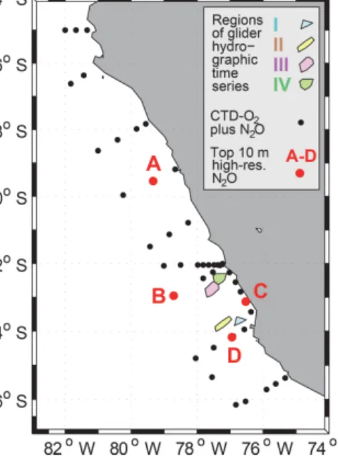
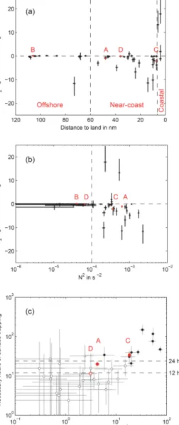
Figure 1.Locations of sample stations and glider time series off the coast of Peru, December 2012 to February 2013. Black dots: simultaneous CTD−O₂and N₂O sampling, comprising 5 and 10 m depth samples, during M91 (3–23 December 2012). Red dots: Zodiac- based high-resolution N₂O profiles of topmost 10 m; A: 8 Decem- ber 2012 at 16:30 local time; B: 13 December 2012 at 10:00 local time; C: 16 December 2012 at 14:30 local time; D: 17 Decem- ber 2012 at 14:00 local time. Colored areas: regions where time series of glider near-surface hydrography were obtained; I: 10 days from 17 to 27 February 2013; II: 22 days from 23 January to 22 February 2013; III: 31 days from 15 January to 15 February 2013;

IV: 37 days from 11 January to 17 February 2013.

depth–oxygen (CTD−O₂, Krahmann and Bange, 2016) and discrete samples of N₂O (Kock and Bange, 2016) were collected (Fig. 1). These data were used to estimate the near- surface vertical N₂O gradient, the stratification between 10 and 5 m, the thickness of the top layer (see Sect. 2.2.3), and the depth of the OMZ upper boundary – here defined by a 20 µmol kg⁻¹oxygen threshold. The latter served to approxi- mately locate the periphery to anoxic conditions, with a sharp oxygen gradient and with expected strong local N₂O production, henceforth referred to as the “oxygen interface”. Four vertically high resolution N2O profiles of the top 10 m were measured from a drifting Zodiac positioned at least 1 km away from the research vessel (Fig. 1). The Zodiac sampling aimed at identifying near-surface N2O gradients not affected by ship-induced turbulence. The top 1 m was sampled by a submersible centrifugal pump with radial intake, providing water at a rate of about 0.5 L min⁻¹. For the water column from 1 to 10 m a manually triggered 5 L Niskin bottle was used, accompanied by a MicroCat to record pressure, temperature, and salinity.

During December 2012, N₂O concentrations at 5.5 m were measured continuously from the ship’s moon pool and are used in this study to complement the Zodiac high-resolution

N2O profiles. In order to estimate N2O 5.5 m concentrations on the station, only values obtained near the station were considered when the vessel was steaming, to avoid disturbances of the water column by the ship’s maneuvering and dynamic positioning. The water temperature at the thermosalinograph intake at the ship’s hull (at 3 m depth) together with the vertical displacement of the intake was used to create an along- track time series of estimated near-surface stratification, in order to explore the link between strong near-surface stratification events and N₂O gradients. Further, a campaign with seven gliders in January and February 2013 (Thomsen et al., 2016) provided undisturbed near-surface hydrographic data with high temporal coverage for four local areas (Fig. 1). For these areas which are characterized by different wind conditions and different distances to land, 1 h resolution time series of stratification in the top 12 m could be composed. These time series served to estimate the occurrence and characteristics of multi-day near-surface stratification, and to force a simple one-dimensional gas-transfer model of the top 12 m of the water column, aimed at producing time series of N₂O distribution and outgassing for different stratifications and wind conditions.

2.2 Sample and data processing 2.2.1 N₂O concentrations

For the discrete N2O measurements, 20 mL water samples were taken (three replicates per depth during CTD−O2casts, six replicates per depth during high-resolution profiles). Fol- lowing Kock et al. (2016), the samples were analyzed on board by gas chromatography with an electron capture de- tector (GC-ECD) after bringing a helium headspace to static equilibrium. The measurement uncertainty was estimated for each profile separately, from the distribution of residuals around the average profile, and lay typically in the range of 0.5 to 1 nmol kg⁻¹(95 % level) for the high-resolution profiles and in the range of 0.5 to 4 nmol kg⁻¹(95 % level) for the CTD profiles. N₂O was also measured from a continuous seawater supply (pumped from 5.5 m depth) with a cav- ity enhanced absorption spectrometer coupled to a seawater and gas equilibrator (Arévalo-Martínez et al., 2013). The re- sponse time of the equilibrator was 2.5 min (translating to a space scale of 750 m at a ship speed of 10 knots). The accuracy of 3 min averages is<0.5 nmol kg⁻¹. A possible in- strument drift, which is typically lower than 1 % per week, was corrected by a 6-hourly calibration of the measurement system (Arévalo-Martínez et al., 2013).

2.2.2 CTD−O₂

Salinity, temperature, and oxygen profiles were obtained from a lowered SeaBird 911plus CTD with dual conductivity and temperature sensors, plus added membrane-type oxygen sensors. Salinity was calibrated against water sam-

(5)

ples analyzed with a Guildline AutoSal salinometer. Oxy- gen was calibrated against water samples using a Winkler titration stand. No further calibration of temperature sensors was performed. Accuracies are 0.002 K in temperature, 0.002 in salinity, and 1 µmol kg⁻¹in oxygen for concentrations≥5 µmol kg⁻¹. We also used temperature profiles derived from a microstructure probe which was equipped with a Pt100 temperature sensor and a thermistor. The gliders carried unpumped CTDs that required a special treatment. Fol- lowing Thomsen et al. (2016), the flow through their conductivity cells was derived from a glider flight model, a thermal lag hysteresis correction was applied, and derived temperature and salinity values were further calibrated against shipboard CTD data from stations close to the glider position.

Accuracy (rms) is 0.01 K in temperature and 0.01 in salinity.

2.2.3 Thickness of the top layer

We will use the term “top layer” (TL) to refer to that layer which ranges from the ocean surface down to a layer of strong stratification, and whose interior is characterized by a relatively weak stratification or even homogeneity. In ex- treme cases when strong stratification extends to the surface, a TL will not exist. Using a new term instead of “mixed layer” or “mixing layer” avoids misunderstandings, as the va- rieties of definitions and criteria for the latter terms are am- ple: sometimes the TL might rather match the mixed layer, and sometimes the TL might better match a temporal mixing layer within the mixed layer. We use the top layer to describe the layer of trapped water, and its thickness or “top-layer depth” (TLD) to describe the depth below which turbulent mixing is suppressed. Therefore we define the TLD based on a criterion relevant for the trapping process. The TLD is at the transition from the TL to the layer of suppressed mixing, and matches the “trapping depth” of Price et al.

(1986), Fairall et al. (1996a), and Prytherch et al. (2013), who considered surface trapping by the diurnal warm layer cycle. Reported criteria are based on the argument that the trapping depth is set by self-regulation between the compet- ing effects of stratification and shear instability and comes to sit where the gradient Richardson number (Ri) is about critical (Price et al., 1986; Fairall et al., 1996a; Prytherch et al., 2013; Soloviev and Lukas, 2014). Reported Ricrite- ria are 0.25 and 0.65, typical shear at trapping depth is 0.5 to 2×10⁻²s⁻¹(Prytherch et al., 2013) or 1×10⁻²s⁻¹(Wene- grat and McPhaden, 2015), both derived from observations of diurnal warm layers. These values correspond to an N² range of 10⁻⁵ to 10⁻⁴s⁻² and match theN²range at trapping depth observed by Wenegrat and McPhaden (2015). We define TLD as the minimum depth where N² ≥10⁻⁴s⁻², in order not to underestimate the trapping depth, and not to overestimate the resulting effects. Calculating TLD this way requires reliable density profiles up to the surface, which are provided by the glider hydrographic surveys during January–

February 2013. In contrast, the shipboard CTD profiles taken

in December 2012 are much less reliable in the top 10 m, because the ship’s engines and maneuvering before and during CTD stations causes overturns and turbulence. This is also the reason why shipboard CTD data usually do not show near-surface density gradients of the same strength as we found in the glider data. Due to the lack of reliable density data, for the ship CTD data we use an auxiliary but more ro- bust criterion. It is based on the temperature difference to the surface and was originally intended for mixed layer detec- tion; cf. Schlundt et al. (2014). The temperature profiles from the shipboard CTD were complemented by collocated temperature profiles from the microstructure probe to reduce uncertainty. To reduce the effect of ship-induced turbulence and under the assumption that any unstable stratification is artifi- cially generated, the measured temperatures of the top 10 m were sorted, with the highest temperatures at the surface.

The depth criterion applied is a density increase compared to the surface which is equivalent to a temperature decrease of 0.5^◦C, while salinity is kept constant (Schlundt et al., 2014).

This alternative top-layer thickness estimate will be referred to as surface layer depth, to illustrate that it is methodically different from TLD.

2.2.4 Estimate of stratification at 3 m depth

We used the water temperature measured at the thermosalinograph inlet near the ship’s bow at nominal 3 m depth, and the vertical movement of the inlet position relative to the water column, in order to derive estimates of the stratification at about 3 m depth while the ship was cruising. This was inspired by the strategy of scanning the near-surface range with bow-mounted sensors by Soloviev and Lukas (1997). As the actual wave height and phase time series are unknown, the inlet position is calculated relative to the mean sea level, defined as average water level relative to the ship in the immediate vicinity of the ship. The vertical distance of the inlet relative to the mean sea level was estimated by rotating the vector of distance of the inlet relative to the ship’s center of mass – first rotating around the ship’s pitch axis, then around the ship’s roll axis, resulting in

dinlet/sealevel ≈ −x_inlet/com·sinπ+ y_inlet/com·sinρ (4)

−zinlet/com·cosρ)·cosπ+dcom/sealevel, with(x, y, z)inlet/comas inlet position relative to the center of mass in ship coordinates,xpositive to bow,ypositive to starboard,zpositive up,ρroll angle positive for starboard down, π pitch angle positive for bow up, anddcom/sealeveldistance of center of mass to sea level. Heave is not part of the transformation because it is assumed that the ship’s center of mass moves only negligibly relative to the mean sea level. The transformation is further only approximate because vertical displacement of the water column at 3 m from wave orbitals or a possible correlation ofdinlet/sealeveland actual sea level at the inlet position could not be taken into account. As the

(6)

time series of recorded data of temperature and vertical position are not reliably synchronous, the vertical temperature gradient is estimated by the square root of the temperature variance divided by the square root of the vertical distance variance. The used variances are variances of residuals relative to a 200 s low pass. The entire procedure assumes that the temperature variance is dominated by the vertical temperature gradient. However, horizontal temperature variability on short scales, vertical movements of the water column, and sensor noise add to temperature variance. The salinity required to convert the temperature gradient into stratification is taken from the thermosalinograph record, using the average salinity during the respective time bin, i.e., assuming a vertical salinity gradient of zero. After having calculatedN² at 3 m depth for the entire cruise, we find an apparent lower limit for N² of about 10⁻⁵s⁻², which is probably caused by the temperature variance which is not due to the vertical temperature gradient. The derived N² time series is not used quantitatively due to the described limitations, but al- lows spatiotemporal variations in near-surface stratification to be qualitatively identified.

2.2.5 Wind speed at 10 m and cloud radiation

Wind speed at 10 m height was needed to estimate gas exchange fluxes. The 10 m wind speed during the ship cruise was derived by converting the wind speed measured at 34 m height at the ship using the COARE algorithm for non- neutral atmospheric conditions (Fairall et al., 1996b). The 10 m wind is the wind speed that exerts the same wind stress on the water surface as the measured 34 m wind, under the measured atmospheric conditions. In order to account for the integrated effect of the varying wind in the gas exchange estimates, wind speed was rms averaged using a cutoff radius in time and space of 6 h and 5 nm, respectively, around the time and position of N₂O sampling. The averaging scales had been chosen after inspecting the continuous N₂O record for typical spatial scales of variability during cruising and for typical scales of temporal variability at the station. Av- eraging was quadratic in order to estimate an effective wind speed that induces the same transfer velocity as the integrated time series of varying transfer velocities, acknowledging that transfer velocities can be well described as proportional to wind speed squared in the lower to medium wind speed range (Garbe et al., 2014), a range that was encountered during most of the cruise (Fig. 2). For the glider time series we used (1) daily wind fields from Metop/ASCAT scatterometer retrievals (http://cersat.ifremer.fr, last access: 28 May 2019;

Bentamy and Croize-Fillon, 2012) that were interpolated to the positions of the gliders, and (2) wind speed from collocated ship records (distance<0.3^◦) that was allocated to parts of the glider hydrographic time series, i.e., only when the ship was nearby. For the latter positions, the long wave radiation (LWR) attributable to cloud cover was also calculated, from incoming LWR minus clear-sky LWR. These

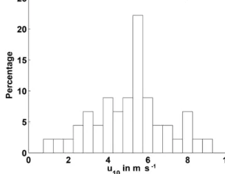
Figure 2.Histogram of rms averaged wind speed in December 2012 at stations where CTD−O₂and N₂O were sampled simultaneously.

Averaging at maximum during 6 h and in a radius of 5 nm around the CTD location.

ship-based observations of wind and cloud-caused LWR will serve to investigate conditions for multi-day near-surface stratification, but due to the gaps in the data they cannot serve to force the N₂O gas-transfer model of Sect. 2.2.7.

2.2.6 N₂O flux densities by air–sea gas exchange, and relative flux error

In order to estimate the N2O flux density (nmol m⁻²s⁻¹) from or to the ocean, the bulk flux parameterization of Nightingale et al. (2000) was used with a Schmidt number exponent ofn= −0.5. The transfer velocity here only de- pends on wind speed with a quadratic law, and is of medium range within the multitude of transfer velocity parameterizations (Garbe et al., 2014). We also calculate a relative flux error (similar to Soloviev et al., 2002) which quantifies the bias that emerges when the flux density is not calculated based on a proper bulk concentration but instead on a differing concentration somewhere in the near-surface layer:

R=8_ns−8_bulk 8bulk

= 8_ns 8bulk

−1= c_ns−c_eq cbulk−ceq

−1, (5) with8bulkthe flux density based on bulk concentrationcbulk, 8nsthe flux density based on concentrationcns, andceqthe concentration in equilibrium with the atmosphere.ceq was calculated following Weiss and Price (1980), using an N₂O mole fraction in dry air of 325 ppb.R can be interpreted as the overestimation percentage of the gas exchange rate if the estimate is based on a concentrationc_ns. The advantage of this relative measure of bias is that it shows the impact of the 1c sampling issue in a clear way independent of the actual value of the transfer velocity and its issues, and ab- stracting from the actual concentration level of the local N₂O profile. Certainly, transfer velocities and N₂O concentrations

(7)

will have to be taken into account when estimating the integrated effect of near-surface stratification on regional emission rates.

2.2.7 One-dimensional gas-transfer model of the surface trapping mechanism

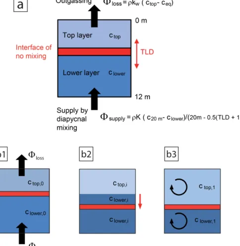
Here we investigate whether the observed vertical near- surface N₂O gradients can principally be caused by near- surface stratification alone. Further, we want to compare the impact of multi-day near-surface stratification versus the impact of just diurnal episodes of near-surface stratification. For these purposes, a model is used which simulates the surface trapping mechanism in a straightforward and simplified manner by vertical one-dimensional transport processes (Fig. 3). The model represents the top 12 m of the water column and takes into account N₂O supply from below, air–sea gas exchange at the surface, and the suppressed mixing that is caused by a thin near-surface stratified layer. That thin stratified layer is simplified to be an interface of complete mixing inhibition, which divides the water column into two separate layers. The two layers (top layer and lower layer) are idealized to be each immediately and completely mixed.

The interface of complete mixing inhibition represents the TLD and can shift up and down in the water column, independent of water movements. That means that the top and lower layers can change thicknesses and entrain water of each other, which leads to the exchange of N2O between the layers (Fig. 3b1–b3). For our purposes, the model needs to be constrained by realistic fluxes and high-resolution time series of TLD data, representative for the conditions in the Peruvian upwelling regime. In particular the TLD time series require attention, as on the one hand locating the TLD needs undisturbed high-resolution information on the top meters of the water column, and on the other hand the temporal resolution must be fine enough to catch the principal TLD shifts through the hours of the day. In particular the expected TLD maximum in the morning and the TLD minimum in the after- noon should be reliably resolved. We use observational data from four locations in the upwelling regime (regions I, II, III, IV in Fig. 1). The locations represent different grades of near-surface stratification, from domination by diurnal episodes to domination by multi-day events. The corresponding four time series of TLD are obtained from glider hydrographic near-surface profiles in January–February 2013 (see Sects. 2.1, 2.2.2, and Thomsen et al., 2016), as they represent undisturbed near-surface data of high spatiotemporal resolution. Time series of hourly density profiles in the top 12 m were assembled from shorter time series of different gliders that were passing through regions I to IV. The density time series were then low-pass-filtered (12 h half power, 3 h cut off) to remove density changes that are only caused by vertical movements of the water column due to internal waves and would otherwise cause spurious exchange between the two layers. TLD was determined as the shallowest

depth where stratification was stronger thanN²=10⁻⁴s⁻² (see Sect. 2.2.3). Air–sea gas exchange was calculated via the Nightingale et al. (2000) parameterization from the actual simulated N₂O concentration of the top layer, fromc_eq based on surface temperature and salinity of the glider hydrographic data, and from transfer velocity calculated from wind speed (see Sect. 2.2.5). N₂O supply from below was determined based on the assumptions that observed N₂O concentrations at 20 m depth can be treated as steady-state and thus are understood as constant boundary values, and that N₂O transport into the lower layer is by turbulent mixing. Actual 20 m concentrations were taken from discrete N2O profiles of December 2012 that were both near regions I to IV and situ- ated at land distances that corresponded to those of region I to IV. Chosen values were 50, 30, 40, and 60 nmol kg⁻¹, respectively. The supply flux density was then calculated as 8=ρ·K· ∇N₂O withρwater density,Kvertical exchange coefficient, and∇N₂O vertical gradient of N₂O concentration. The N₂O gradient is the difference between 20 m concentration and the concentration in the lower layer, divided by the distance between 20 m and the temporary center depth of the lower layer. In order to get an estimate of the range of the vertical exchange coefficientK, K was determined from microstructure measurements at stations where strong shallow stratification between two weakly stratified layers was clearly present. There, vertically averagedKwas determined for the depth range from below the TLD down to 20 m.

For details ofKestimation from velocity microstructure see Fischer et al. (2013). The observed K values ranged from 10⁻⁵m²s⁻¹to near 10⁻²m²s⁻¹with median 10⁻⁴m²s⁻¹ and mean 10⁻³m²s⁻¹. After having chosen a value forK and which region (I to IV) was to be simulated, the model is forced by cyclic application of according wind and TLD time series until cyclic equilibrium. As a result, the model produces time series of N₂O concentration vs. depth, so that time series of measurement biasRvs. depth can be obtained and compared to observations.

3 Results

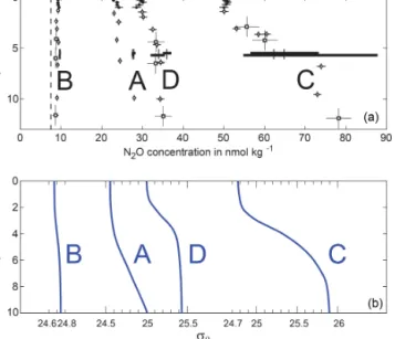
The four off-ship high-resolution N2O profiles (A to D) that were unaffected by ship-induced stirring show that near- surface N2O gradients do generally exist in the Peruvian upwelling region (Fig. 4). The N2O gradients, which are of vari- able strength but all downward or zero, are located below a thin homogeneous top layer of 1 to 5 m thickness. The N₂O gradients strengthen with decreasing distance to the coastline and weakening winds. They are very similar in shape to the corresponding density profiles, i.e., a stronger N₂O gradient is also associated with stronger stratification.

Discrete N₂O samples from the closest shipboard CTD profiles are consistent with the off-ship profiles, despite some distance in space and time. The N₂O data – taken while ap- proaching or leaving a station – are from a distinctly larger

(8)

Figure 3. (a)The one-dimensional gas-transfer model to simulate the surface trapping mechanism. The interface of complete mixing inhibition shifts up and down according to the high-resolution time series of observed TLD without instantaneously affecting local N₂O concentrations. Vertical N₂O transport is achieved by mixing within the two layers after the shifting interface has left a portion ofc_lower water in the top layer, or vice versa. Panels(b1–b3)demonstrate the processing sequence during a model time step.(b1)For the duration of the time step, supply flux and outgassing flux changec_topandc_lower, resulting in intermediate concentrationsc_top,iandc_lower,i.(b2)After the time step, the TLD is shifted, in the example to a greater depth.(b3)Instantaneous linear mixing within the new top and lower layers results in concentrationsc_top,1andc_lower,1, which serve as start values for the next model time step.

distance in space and time than the discrete N₂O samples and vary more, though still match the general pattern. Par- ticularly at site C the data based on continuous sampling span the entire concentration range of the top 10 m of the off- ship high-resolution profile. The consistency of off-ship, discrete, and mean N2O concentrations from continuous sampling suggests larger regions of at least some nautical miles’

extent to be basically horizontally homogeneous in the top 10 m, while the variability of the continuous N₂O concentrations particularly at site C suggests that vertical motions (most likely due to internal waves) are superposed, transfer- ring water from different nominal depths to the sample inlet at 5.5 m. Such variability is not visible in the discrete N₂O samples of profile C, because these were projected onto the mean density profile which was observed during the off-ship sampling. So profile C does explicitly not show variability

caused by internal wave motion, which was strong in the top meters at that site.

In order to further explore the spatial distribution and the conditions that lead to near-surface N₂O gradients, the data set was complemented by the topmost ship-based N2O samples collected during December 2012. By taking into account these data, we accept the enhanced uncertainty in allocat- ing N2O concentrations to depths which arises from ship- induced disturbances in the top 10 m of the water column.

On the other hand we have shown a consistent behavior of off-ship and shipboard N₂O samples at sites A to D. The ship-based data allow the N₂O difference between about 5 and 10 m depth to be examined. This provides a data set of 45 near-surface N₂O gradient estimates, as plotted in Fig. 5a as a function of distance to land. The encountered N₂O gradients are mostly downward, i.e., negative with the convention of thezaxis pointing upward, but occasional upward (positive)

(9)

Figure 4.N₂O and density profiles at the off-ship high-resolution stations A to D, complemented by shipboard observations at adja- cent positions and times. For positions and times of station A to D see Fig. 1. Distances to land – B: 106 nm; A: 48 nm; D: 36 nm;

C: 7 nm. 95 % limits of 10 m wind distribution in meters per sec- ond (m s⁻¹): B [4.3 6.6], A [3.1 6.0], D [2.6 5.9], C [3.3 5.4].

(a)N₂O measurements with 95 % confidence limits from measurement uncertainty; black dots in top 1 m: samples from centrifugal pump off-ship; black circles below 1 m: samples from Niskin bottles off-ship; black squares: samples from shipboard CTD; thick black lines: 95 % limits of distribution of continuous ship samples during approach and departure of the station, median values are marked.

(b) Density profiles derived from MicroCat temperature and conductivity profiles at stations A to D.

gradients occur very close to the coast. Far off the coast, gradients are mostly insignificant. The compilation shows that even stronger N₂O gradients exist than observed at the off- ship high-resolution stations and suggests a zoning into neutral (“no”) gradients off 60 nm, downward gradients between 60 and 6 nm, and upward gradients inland of 6 nm. These zone limits are peculiar for the sampling depth between 5 and 10 m and would probably take different values for gradients at other sampling depths. Note that the profiles’ behavior at depths shallower than 5 m is unknown here, so we cannot exclude that profiles of upward gradient between 5 and 10 m still exhibit a downward gradient in the top meters. Note as well that the high-resolution profiles tended to not exhibit their strongest gradients between 10 and 5 m, suggesting that stronger gradients than those shown in Fig. 5a may exist. The single occurrence of a strong N₂O gradient 70 nm offshore coincides with a shallower mixed layer and less oxygen below the mixed layer than expected at that open-ocean location. The sea surface temperature field at the time of sampling shows a filament reaching from the coast to the station position. Those aspects suggest that coastal water with

a downward N2O gradient has been transported to the open ocean.

Elevated N₂O gradients (downward and upward) are con- fined to strong stratification (Fig. 5b), with a threshold buoyancy frequency of aboutN² =10⁻⁴s⁻². Following the argu- ments in Sect. 2.2.3 that during surface trapping the trapped top layer is isolated from waters below by already somewhat weaker stratifications ofN²between 10⁻⁵and 10⁻⁴s⁻², this indicates that the strong N₂O gradients are associated with surface trapping.

A question to address here is how much time would be needed to form the observed N2O gradients by surface trapping and air–sea gas exchange. The shipboard discrete N2O data allow a rough estimate for the majority of profiles with significant gradients, namely the downward ones, with 5 m concentration<10 m concentration (Fig. 5c). The calcula- tion assumes an initially homogeneous N₂O distribution in the upper 10 m. Then, the top 5 m are trapped and get de- pleted by air–sea gas exchange, until the observed 5 m concentrations are reached. Horizontal N₂O transport and N₂O supply from below are not accounted for. Thus, the N₂O concentration difference between 5 and 10 m is an N₂O deficit that developed during the hours of isolation of the top 5 m, assuming the wind conditions encountered during station sampling. Taking into account that we expect the top 5 m to exhibit a downward or neutral gradient (cf. Fig. 4), the N2O deficit calculated in this simple approach is actually expected to be a lower bound to the real amount of N2O that has been emitted. Together with the assumption of no-N2O supply from below, the calculated time spans represent an underestimate of the necessary duration of surface trapping.

The strongest quarter of N₂O gradients in Fig. 5c needs isolation periods of distinctly more than 24 h, i.e., multi-day near- surface stratification, and there are some other strong gradients with isolation periods shorter than 24 h that nevertheless still comprise the entire previous night. Profiles of upward gradient between 10 and 5 m will be discussed in Sect. 4.3.

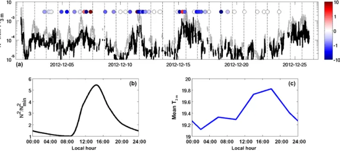
The suggestion that multi-day near-surface stratification exists and is not rare, and that it is associated with the strongest near-surface N₂O gradients, is further supported by additional observations. Figure 6 aligns the shipborne along-track time series of estimated N² at 3 m depth during December 2012 with the observed N2O gradients. The time series of 3 m stratification shows a distinct diurnal cycle with maximum stratification around 15:00 local time. We aimed to subtract that diurnal cycle of near-surface stratification, in order to mimic a time series of the local nighttime N² minimum, and in this way detect locations where near- surface stratification probably survived the previous night and can be called multi-day near-surface stratification. Inter- estingly, the diurnal cycle is much better removed in logarith- mic space than in linear space; so we calculated a mean diurnal cycle of log₁₀N², scaled it with an offset such that the minimum of (log₁₀N²+offset) equals zero, and then subtracted this scaled mean diurnal cycle from the time series of

(10)

Figure 5.Characteristics of shallow N₂O gradients derived from shipboard samples. The N₂O gradient is calculated from bottle samples at about 5 m and about 10 m depth; negative gradients are defined as concentration decreasing with vertical coordinatezor increasing with depth. Error bars are 95 % confidence limits based on measurement uncertainty. Red symbols are high-resolution stations A to D (see Figs. 1 and 4).(a)N₂O gradient vs. distance to land, calculated as shortest distance to coast. Dashed vertical lines separate three zones (offshore, near-coast, coastal), dominated by neutral, downward, and upward gradients, respectively.(b)N₂O gradient vs. buoyancy frequency squared,N², calculated from densities of the corresponding N₂O bottle samples. The dashed vertical line atN²=10⁻⁴s⁻²marks the approximate threshold below which no strong N₂O gradients occur.(c)N₂O deficit vs. estimated necessary time span of surface trapping, N₂O deficit is concentration difference between 10 and 5 m; hours of isolation are the time needed to deplete a 5 m water column from the 10 m concentration down to the 5 m concentration. Filled circles are stations where the necessary isolation time includes minimum one entire night, even for the lower confidence limit. Open circles are stations where night mixing cannot be excluded. Station B showed no negative gradient and is not part of the plot.

log10N². The nonlinearity of the diurnal evolution of near- surface stratification might be due to the fact that preexisting stratification will suppress turbulent mixing and increasingly promote surface trapping of heat during the daytime, thus acting to self-perpetuate. The presence of surface trapping is also revealed by the mean diurnal cycle of temperature at 3 m (Fig. 6), with a mean amplitude of 0.6 K. Figure 6 shows that the strongest N₂O gradients come in three clusters (i.e., around 5, 10, and 15 December, respectively), and they are associated with minimum nighttime stratification on the order ofN² =10⁻⁴s⁻², which is strong enough to assume surface trapping (Sect. 2.2.3). The clusters suggest the existence of larger regions of multi-day near-surface stratification that have been crossed during the cruise. Direct observational evidence for multi-day near-surface stratification in the form of stratification time series in fixed regions comes from four local hydrographic time series obtained during the glider campaign in January–February 2013 (Fig. 7). The time series in regions I to IV (see Fig. 1) show different grades of persistence of near-surface stratification, ranging from a classic diurnal warm layer periodicity with regular nighttime mixing (I) to a strong stratification layer not retreating deeper than 2 m from the surface for several days in a row (IV).

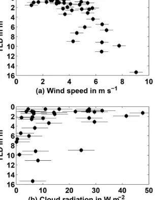
Conditions that promote the occurrence of multi-day near- surface stratification were examined for the glider data on nights when glider positions and ship positions were collocated (distance≤0.3^◦ in latitude and longitude), so that wind speed and long wave radiation from clouds could be as- signed to thicknesses of the homogeneous top layer (Fig. 8).

The data show that at low to moderate wind (0 to 6 m s⁻¹) it is possible to find near-surface stratification persisting all night, the main prerequisite of multi-day near-surface stratification. Below wind speeds of 3 to 4 m s⁻¹multi-day near- surface stratification even seems certain. Additional cloud cover supports the persistence of near-surface stratification.

Unfortunately the glider time series could not be accompanied by N₂O measurements, so that a co-occurrence of the glider-observed periods of multi-day near-surface stratification with a progressing formation of strong N₂O gradients can only be tested in a modeling framework. We use the 1- D gas-transfer model introduced in Sect. 2.2.7, simulating within its simple setup the surface trapping mechanism and the formation of N2O gradients. The model is forced with the glider time series of TLD and with ASCAT daily winds. Fig- ure 9 shows N2O distributions as a function of depth which result from the model runs with applied forcings of region I to IV, displayed as distributions of relative flux errorR or flux overestimation (Sect. 2.2.6).Ris insensitive to the actual N₂O supply from below, both for the range of assumed 20 m concentrations and for the range of vertical turbulent diffu- sivity from 10⁻⁵ to 10⁻²m²s⁻¹. This insensitivity is plau- sible, becauseR can be expressed as ^c_c^ns^−c^bulk

bulk−ceq,(c_ns−c_bulk) is proportional to the N2O flux from the lower layer (with cns) to the top layer (withcbulk),(cbulk−ceq)is proportional

(11)

Figure 6. (a)Observed near-surface N₂O gradients vs. stratification at 3 m, in December 2012. Grey line:N²at 3 m estimated from hull temperature variance and ship motion variance; data gaps are during ship stations. Diurnal periodicity is visible most days. Black line: same with mean diurnal cycle subtracted, by that mimicking the expected minimum nighttime stratification at each location. Colored dots: N₂O gradient between about 10 and 5 m depth from ship-based discrete sampling. Dashed lines mark 15:00 h local time.(b)Mean diurnal cycle of stratification at 3 m, relative to minimum nighttime stratificationN_min² .(c)Mean diurnal cycle of temperature at 3 m.

Figure 7. Near-surface stratification in composite glider hydrographic time series, sorted by increasing grade of persistence, from that dominated by the diurnal cycle to that dominated by multi-day events. I, II, III, IV: regions of glider time series (Fig. 1). Black line:

minimum depth ofN²≥10⁻⁴s⁻², as base of the top layer (TLD, Sect. 2.2.3). Time series are composites of different, partly overlapping glider sections in respective regions. All four time series are from January–February 2013; their exact dates can be obtained from Fig. 1.N² processed in 0.5 m vertical bins, after low-pass-filtering the hydrographic time series (half powerk=(12 h)⁻¹, cutoff (3 h)⁻¹) to eliminate spurious variations of TLD caused by internal wave vertical motions.

(12)

Figure 8.Influence of wind speed(a)and cloud radiation(b)on nighttime near-surface stratification. Night TLD is the night average from glider hydrographic time series (Fig. 7). Wind speed is the night rms average of ship wind from collocated positions (distance

≤0.3^◦lat. and long.), converted to 10 m wind under non-neutral conditions using the COARE algorithm. Cloud radiation is the night average of long wave radiation minus clear-sky long wave radiation.

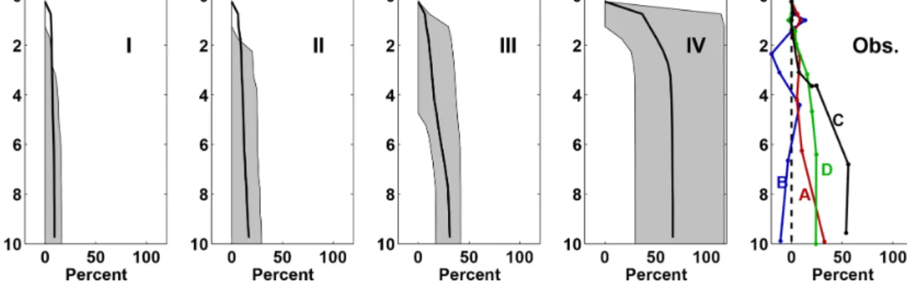
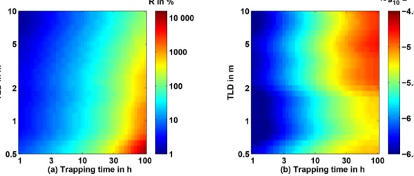
to the N2O flux from the top layer to the atmosphere, and in the model equilibrium both fluxes are equal on average. This way, expressed asR, modeled N2O gradients can be advan- tageously compared to observed gradients without consider- ing the magnitude of supply flux. It is just the impact of surface trapping on gradient formation that is compared between model and observed N₂O profiles. The results in Fig. 9 show that the model produces distributions ofRthat comprise the observedR of the high-resolution N₂O profiles; i.e., the observed N₂O gradients during December 2012 are within the range that was modeled in accordance with observed surface trapping scenarios. An increase in the number of multi-day events in the TLD time series I to IV leads to increasingly higherRvalues; i.e., increasingly stronger N2O gradients are expected on average.

4 Discussion

4.1 The role of multi-day near-surface stratification for near-surface gas gradients

We will argue here that multi-day persistence of near-surface stratification is able to explain the formation of strong near-

surface gas gradients, and furthermore that it is unlikely to achieve strong gas gradients through near-surface stratification on shorter timescales. The basic linkage of near- surface stratification and vertical gradients of any property in the near-surface ocean has been established (particularly plainly stated by Soloviev and Lukas, 2014) and is attributed to turbulence suppression in the temporally stratified layer, i.e., to surface trapping. However, studies dealing with consequences of near-surface stratification generally focus on short timescales, usually on the diurnal warm layer cycle (Soloviev et al., 2002; Kawai and Wada, 2007; Gentemann et al., 2009; Wenegrat and McPhaden, 2015). Prytherch et al.

(2013) mention the possibility of preexisting stratification at sunrise (i.e., incomplete erosion of stratification during the night and longer timescales of near-surface stratification are implied), and observe subsequent amplification of surface warming, but they do not explore further consequences. Our database and results allow the view to be extended to the multi-day timescale. In this respect our results show, firstly, that multi-day near-surface stratification in the Peruvian upwelling region is not rare, lasts up to several nights in a row, and that remaining stratification at sunrise is strong of or- derN²=10⁻⁴s⁻²and more (Fig. 7). Conditions which support the endurance of stratification through the night and thus multi-day timescales are basically the same as those that promote near-surface stratification on shorter timescales, that is, low wind energy input and low heat loss (Fig. 8). Secondly, observations show that the absolute near-surface N2O gradient is positively related to the strength of near-surface stratification (Figs. 4, 5b), such that the observation that multi-day stratification is abundant and strong results in the expectation of associated abundant and strong N₂O gradients. Thirdly, the duration of near-surface stratification can also be directly related to the strength of near-surface N₂O gradients. This is indicated by three lines of observations and analyses. (i) Dur- ing the cruise in December 2012, clusters of multi-day stratification coincided with clusters of the strongest N₂O gradients (Fig. 6). (ii) When estimating necessary trapping times to produce observed N₂O gradients (Fig. 5c), the strongest quarter of gradients can only be caused by multi-day trapping. (iii) When on the other hand estimating N₂O gradients caused by observed trapping conditions (process model with observed TLD time series; Fig. 9), strong gradients become more and more likely with more frequent occurrences of multi-day stratification events.

Until here, the line of evidence supports the hypothesis that multi-day near-surface stratification can explain strong near-surface N₂O gradients. To go beyond this, Figs. 5c and 9 and also the results of Soloviev et al. (2002) suggest that substantial gas gradients are not only made possible by but even need trapping times beyond the typical up to 12 h of the diurnal warm layer cycle. “Substantial” is unfortunately vague here, because the strength of gradients cannot be directly compared between the figures. Figure 9 indicates that region I which is dominated by the diurnal cycle is good for

(13)

Figure 9.Modeled and observed N₂O profiles, expressed as relative flux errorR(Sect. 2.2.6), i.e., equivalent to overestimation of air–sea gas exchange flux if using N₂O at depth instead of bulk N₂O in bulk flux parameterizations. I, II, III, IV: distributions ofRin runs of 1-D transport model (Sect. 2.2.7), forced by time series of TLD from respective glider time series, and by ASCAT wind speed. Thin lines/grey shading:

95 % limits of temporal distribution of flux overestimation at each depth. Thick lines: mean flux overestimation. OBS: flux overestimation of observed high-resolution profiles at sites A to D.

a typicalRof 10 %, while region IV, which is dominated by multi-day near-surface stratification, exhibits R of 50 % to 100 %. The transition between diurnal and multi-day stratification cycles may be seen in regions II and III withRabout 30 %. This is in line with Soloviev et al. (2002), who find a maximum R of 30 % in their investigation of gas gradients caused by the diurnal warm layer cycle. For the gradients of Fig. 5c, information on concentrations above 5 m depth is lacking, so R cannot be calculated. However, we can still roughly estimate R by using the concentration at 5 m forc_bulk, and using the concentration at 10 m forc_ns, as is done in Fig. 10. This results in a threshold forRof 30 % to 50 %, above which gradients can only be achieved by multi- day near-surface trapping. Overall, these three independent estimates indicate that near-surface stratification at diurnal timescale can only account for gradients worthR=30 % or less.

Can we understand better why the trapping time seems to play such an important role for gradients? Other factors such as TLD and wind speed are involved in the effective- ness of the surface trapping mechanism, but it seems they only occur in combinations which lead to necessary trapping times on multi-day scales in order to cause substantial N₂O gradients. To gain some insight, we examine the formation of downward N₂O gradients in a very simplified setting and work out the time and TLD dependence of relative emission bias R (as a measure for gradient strength).

An initially homogeneous water column of concentrationc₀, which becomes stratified at the depth TLD at timet₀=0, is assumed. The stratification immediately causes a complete shutdown of N2O supply from below, such that only gas exchange with the atmosphere acts and diminishes the con- centrationcTL in the TL. In the following we will call this simplified process model the “shutdown model”. The difference to the 1-D gas-transfer model of Sect. 2.2.7 is the lack of vertical movement of the TLD, which would per-

Figure 10.Necessary trapping time to explain observed differences between N₂O concentrations at 5 and 10 m, as a function ofR. De- pletion of the top 5 m layer by air–sea gas exchange due to observed wind is assumed. Due to the sparse resolution of N₂O profiles at ship stations,Ris estimated by settingc_bulk=c_{5 m}andcns=c_{10 m}.

mit N2O supply from below through entrainment. Using a bulk parameterization, the outgassing flux density will be 8=kw ·(cTL−ceq), and the change in top-layer concentration with time ^dc_dt^TL = − ⁸

TLD= − ^k^w

TLD ·(c_TL−c_eq). The solution isc_TL=c_eq+(c₀−c_eq)·exp

− ^k^w

TLD ·t

, such that R= c₀−c_eq

cTL−ceq

−1=exp k_w

TLD ·t

−1. (6) The decisive timescale here is^TLD_k

w and the necessary trapping time to reach a certainRis

Ttrap=TLD

k_w ·log(R+1). (7)

Fork_wwe choose the transfer velocity of Nightingale et al.

(2000), which after scaling to the N₂O Schmidt number is a

(14)

Figure 11.Gas exchange overestimationRas a measure of relative gas exchange bias(a)and specific flux biasBas a measure of absolute gas exchange bias(b), both as a function of trapping timeTtrapand top-layer depth TLD. Based on corresponding values of wind speed u₁₀and TLD as observed during the glider mission (Fig. 8), the field ofR(Ttrap,TLD)has been interpolated and smoothed by a Gaussian algorithm. A complete shutdown of N₂O supply to the TL from below is assumed, as is air–sea gas exchange transfer velocity following Nightingale et al. (2000).

function of wind speedu10only:kw= 2

9 ·u²₁₀+¹

3·u10

· _Sc

N2O

600

−0.5

. To estimate trapping timesT_trap as a function of R and TLD, we use TLD from glider observations, and correspondingu10from nearby ship time series, which were already employed to investigate the conditions for multi-day stratification (Fig. 8). DisplayingRas a function ofT_trapand TLD (Fig. 11a) shows that TLD has an effect, butR proves to be more sensitive to changes inT_trapthan in TLD, within the observed range of values. This can be explained by the relation of TLD andk_w(oru₁₀): weaker wind which tends to accompany thinner TL leads to a reduction in gas exchange so that gradient formation is only weakly intensified with decreasing TLD. However, for very thin TL with TLD≤0.5 m, trapping on a diurnal timescale might produce R >30 %.

Unfortunately, this is outside of our observational evidence.

So far we evaluated the strength of gas gradients in terms of relative flux overestimationR. If we want to evaluate the absolute impact of gas gradients on gas flux estimates, the transfer velocity and the actual gas concentration have to be accounted for as well. Keeping the shutdown model that was introduced just above, and defining the absolute flux bias18 as the difference between the flux estimate based on concentrationc₀and the flux estimate based on concentrationc_TL, we get

18=kw ·(c0−ceq)−kw ·(cTL−ceq)

=k_w ·(c₀−c_TL), (8) and using the definition ofR(Eq. 5) to eliminatecTL, 18=kw·R·(cTL−ceq)=kw · R

R+1 ·(c0−ceq). (9)

As there is no data forc0 to accompany the relation be- tweenkw and TLD,18itself cannot be calculated, but we will examine the term

18

c₀−c_eq=kw · R

R+1=B, (10)

which can be interpreted as a specific absolute flux bias per unit supersaturation. ComparingB for different conditions means assuming that c0 is independent of the conditions, while TLD andcTL react to wind speed and trapping time.

Figure 11b shows thatB is practically independent of TLD.

This means that the enhancing effect onBof a stronger gas gradient, which comes with a thinner TL, is fully compen- sated for by the diminishing effect onB of the lower total gas transfer due to the lower wind speed which enabled the thinner TL in the first place.

Thus we may conclude from this subsection that (i) the trapping time is decisive for the formation of gas gradients of high impact on gas exchange estimates (Fig. 11), and building on this, (ii) multi-day near-surface stratification can explain the observed gas gradients (Figs. 7 and 9), while (iii) substantial flux bias is not to be expected from near-surface stratification at diurnal or shorter timescales (Figs. 9, 10, and 11).

4.2 Moderate wind speed causes strongest gas exchange bias

Further using the shutdown model of Sect. 4.1, the timescale

TLD

kw as a function of wind speedu₁₀(Fig. 12a) suggests that there exists an optimum wind range for gas gradient formation. Gas gradients that cause a particular relative gas exchange biasR are reached after a trapping time that is proportional to the timescale ^TLD_k

w (see Eq. 7) and can thus be