Mixed layer depth dominates over upwelling in regulating the seasonality of ecosystem functioning in the Peruvian Upwelling System
Tianfei Xue
1, Ivy Frenger
1, A.E. Friederike Prowe
1, Yonss Saranga José
1, and Andreas Oschlies
1,21GEOMAR Helmholtz Centre for Ocean Research Kiel, Kiel, Germany
2Christian-Albrechts-University Kiel, Germany Correspondence:Tianfei Xue (txue@geomar.de)
Abstract.The Peruvian Upwelling System hosts an extremely high productive marine ecosystem. Observations show that the Peruvian Upwelling System is the only Eastern Boundary Upwelling Systems (EBUS) with an out-of-phase relationship of seasonal surface chlorophyll concentrations and upwelling intensity. This "seasonal paradox" triggers the questions: (1) what is the uniqueness of the Peruvian Upwelling System compared with other EBUS that leads to the out of phase relationship;
(2) how does this uniqueness lead to low phytoplankton biomass in austral winter despite strong upwelling and ample nu- 5
trients? Using observational climatologies for four EBUS we diagnose that the Peruvian Upwelling System is unique in that intense upwelling coincides with deep mixed layers. We then apply a coupled regional ocean circulation-biogeochemical model (CROCO-BioEBUS) to assess how the interplay between mixed layer and upwelling is regulating the seasonality of surface chlorophyll in the Peruvian Upwelling System. The model recreates the "seasonal paradox" within 200 km off the Peruvian coast. We confirm previous findings that deep mixed layers, which cause vertical dilution and stronger light limitation, mostly 10
drive the diametrical seasonality of chlorophyll relative to upwelling. In contrast to previous studies, reduced phytoplankton growth due to enhanced upwelling of cold waters and lateral advection are second-order drivers of low surface chlorophyll concentrations. This impact of deep mixed layers and upwelling propagates up the ecosystem, from primary production to export efficiency. Our findings emphasize the crucial role of the interplay of the mixed layer and upwelling and suggest that surface chlorophyll may increase along with a weakened seasonal paradox in response to shoaling mixed layers under climate 15
change.
1 Introduction
The Peruvian Upwelling System (PUS) hosts a disproportionally productive ecosystem and supports 10% of the world’s fishing yield while covering only 0.1% of the ocean area (Chavez et al., 2008). As one of the Eastern Boundary Upwelling Systems 20
(EBUS), upwelling-favorable winds bring up cool, nutrient-rich waters to the surface, supporting high primary production and
fish yield. At the same time, the high primary production, together with subsequent export and remineralization in part causes a sub-surface oxygen deficient zone which is particularly shallow and intense in the PUS (Fuenzalida et al., 2009; Stramma et al., 2010; Getzlaff et al., 2016). Particularly via its high productivity, the response of the PUS to climate change is of great social and economic interest (Pauly et al., 1998; Bakun, 1990; Bakun et al., 2010), and a variety of studies have investigated 25
how physical and biogeochemical processes influence the production of phytoplankton and its potential links to ecosystem functioning in the PUS.
While the PUS has been frequently compared to other EBUS (the Benguela, California, and Canary Systems), it is set apart by how the surface chlorophyll responds to the variation of upwelling on a seasonal scale. The high productivity of EBUS primarily benefits from the upwelling of nutrient-rich waters, driven by the alongshore equatorward winds. Hence, 30
it is commonly assumed that the magnitude of phytoplankton biomass in EBUS is directly correlated with the wind-driven upwelling intensity (Bakun, 1973). However, in the PUS, upwelling intensity and surface chlorophyll are not correlated on the seasonal scale (hereafter referred to as "seasonal paradox"; Chavez and Messié, 2009). Indeed, they are out of phase, with the lowest surface chlorophyll concentration in austral winter when upwelling intensity is highest (Calienes et al., 1985).
Echevin et al. (2008) and Messié and Chavez (2015) argue that mixed layers are deep when upwelling and nutrient supply is 35
highest. Deep mixed layers would cause dilution of phytoplankton, and growth to be limited by light, and subsequently iron (as phytoplankton needs more iron under low light condition), leading to low chlorophyll under strong upwelling conditions.
Lower surface radiation in winter might amplify light limitation (Guillen and Calienes, 1981). Hence, while upwelling and mixed layer depth both regulate phytoplankton, the interplay of the two has not been assessed. Further, it remains unclear why the seasonal paradox occurs only in the PUS and not in the other EBUS.
40
To this end, this study will address the following key questions: (1) what is the uniqueness of PUS compared to other EBUS that leads to the seasonal paradox; (2) how does the unique mechanism limit phytoplankton from growing under strong upwelling; and (3) how will this further affect ecosystem functioning.
2 Data and Methods
2.1 Regional ocean circulation-biogeochemical model: set up and simulation 45
We use the three-dimensional regional ocean circulation model CROCO (Coastal and Regional Ocean COmmunity model;
Debreu et al., 2012) coupled with the biogeochemical model BioEBUS (Biogeochemical model for the Eastern Boundary Upwelling Systems; Gutknecht et al., 2013) for this study.
We use the same technical set-up including the model grid as in José et al. (2017) with an updated version of the ocean circulation model CROCO. CROCO is a free-surface and split-explicit regional ocean model system (ROMS; Shchepetkin and 50
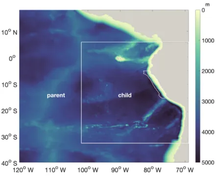
McWilliams, 2005). We employ a two-way nesting approach, with the larger coarser-resolution domain covering the Southeast Pacific and the smaller higher-resolution domain focusing on the PUS. The larger domain has a 1/4◦resolution, spanning from 69◦W to 120◦W and from 18◦N to 40◦S. The embedded "child" domain has a resolution of 1/12◦and extends from 5◦N to 31◦S and from 69◦W to 102◦W (Fig. A1) which is used in this study. Both coarse and fine-resolution domains use 32 sigma
levels in the vertical direction, with finer resolution towards the surface and shallower regions. The surface layer thickness is 55
ranging from 0.5 m in the coastal region (water depth around 50 m) to around 3 m in the offshore region (water depth more than 4000 m). Initial and boundary conditions are provided by the monthly climatological SODA reanalysis (Simple Ocean Data Assimilation; Carton and Giese, 2008) from 1990−2010. The surface forcing is based on the monthly climatological heat and freshwater fluxes from COADS (Comprehensive Ocean-Atmosphere Data Set; Worley et al., 2005), along with wind data from QuikSCAT (Quick Scatterometer; Liu et al., 1998). The physical setup is the same as in José et al. (2017) and 60
has been evaluated therein. The model simulates eddy kinetic energy, sea surface height and alongshore current well, with an underestimation of the intensity of the Equator–Peru coastal current and Peru–Chile undercurrent.
The biogeochemical BioEBUS model used in this study was developed explicitly for applications to EBUS and oxygen minimum zones. BioEBUS is a nitrogen-based model originating from the N2P2Z2D2model by Koné et al. (2005). It simulates two phytoplankton and two zooplankton groups: small and large phytoplankton, along with micro- and mesozooplankton.
65
Further, there are two detritus pools categorized based on size. BioEBUS resolves the N species (nitrate, nitrite and ammonium) and simulates processes under oxic, hypoxic and suboxic conditions (e.g. remineralization, nitrification, denitrification and anammox). Initial and boundary conditions for nitrate and oxygen are from CARS (CSIRO (Commonwealth Scientific and Industrial Research Organisation) Atlas of Regional Seas; Ridgway et al., 2002), and initial conditions for phytoplankton are based on monthly climatological SeaWiFS (Sea-viewing Wide Field-of-view Sensor; O’Reilly et al., 1998) estimates.
70
A detailed description of biogeochemical processes can be found in Gutknecht et al. (2013). The parameter setting is the same as in José et al. (2017), with a few adjustments to biological parameters (Table. A1) to make the ecology, in particular phytoplankton and zooplankton biomass and seasonality, better fit the observations.
CROCO-BioEBUS is run in coupled mode from the start. The time-stepping of the physical model is the same as the coupling timestep, 1200 seconds. The time-stepping of the biogeochemical model is 400 seconds. The coupled model is run 75
for a 25-year spin-up period. Biogeochemical and physical fields are spun-up after one year for the upper 10 m while it takes longer for the deep waters (1000 m) to reach a statistical quasi-equilibrium (Fig. C1). In this study, we use monthly output of the final five years for our analyses (years 26−30). As we look at the surface ecology, our results are not sensitive to the deep spin-up. This study focuses on the 200 km band off the Peruvian coast (white line region in Fig. 1a-b) where shows the clear seasonal variation along with the strong upwelling.
80
2.2 Analyses approaches
To assess the seasonal variance of phytoplankton biomass concentration in each grid box (C) we analyze with the budget of the phytoplankton biomass and how its tendency is driven by physical versus biological processes:
∂C
∂t =P HY(C) +BIO(C) (1)
PHY represents the physical processes including advection and mixing. The BIO term stands for the biological processes, 85
namely primary productionP P, consumptive mortality, natural mortality, exudation and sinking. We analyse in detail the
drivers ofP P:P P is determined by phytoplankton concentration (C) and the growth rate (J)
P P=C·J(N, P AR, T) (2)
where the growth rateJis related to light availability for photosynthesis (PAR: photosynthetically active radiation), temperature (T) and nutrients (N: nitrate, nitrite and ammonium). The growth rate here is a multiplicative function of the light-, temperature- 90
or nitrogen-related growth factors. To quantify the limitation experienced by phytoplankton within the mixed layerLmld, it is calculated from each growth factor (L(PAR),L(T)andL(N)) using phytoplankton concentration (C) within the mixed layer as a weight (Eq. 3). Light-, temperature- or nitrogen-related growth factors that each phytoplankton cell experiences are computed online.
Lmld= Pmld
0 L(PAR)·L(T)·L(N)·C Pmld
0 C (3)
95
For the analysis, we attribute the seasonal change of the average phytoplankton biomass concentration (Cmld) within the mixed layer to the change of the integrated phytoplankton content within the mixed layer (Bmld), and the change of the volume of the mixed layer (Vmld). With the chain rule andV2>> V∆V, we approximate a discrete change of the mixed layer tracer concentration (∆Cmld) with
∆Cmld= 1
Vmld∆Bmld−Bmld∆Vmld Vmld2 =Bmld
Vmld
∆Bmld Bmld −Bmld
Vmld
∆Vmld
Vmld (4)
100
To assess the relative contributions we then divide byCmld=Bmld·Vmld−1to obtain
∆Cmld
Cmld =∆Bmld
Bmld −∆Vmld
Vmld (5)
which allows attributing a decrease of the mixed layer phytoplankton concentrationCmld to a decrease of the phytoplankton biomassBmldor an increase of the mixed layer volumeVmldand vice versa.
2.3 Model assessment 105
The model is evaluated based on averages over the focus region with observational data in monthly resolution. The correlation coefficient between the model simulation and observations, the root mean square error (RMSE) and the normalized standard deviation (SD) of the observations relative to the model results are shown in a Taylor diagram as a summary of the evaluation (Fig. 1c, Taylor et al. (1991); a comparison of the spatial pattern and the seasonal cycles of variables are provided in the appendix, see Figs. B1-B4). Model results fit the observational data reasonably well. The model performs well in simulating 110
sea surface temperature (SST) withR>0.95, 1<σ∗<1.2 andRM SD∗<0.4 (R: correlation coefficient,σ∗: normalized SD, and RMSD∗: normalized RMSD). The model captures the observed seasonal cycle well with slightly stronger seasonal variations compared to observational data. As for MLD (defined based on a 0.2oCtemperature difference criterion), though the seasonal variation is somewhat overestimated, the model simulation is within the observed range of ARGO based MLD most of the time (Fig. B3). As for biogeochemical variables, the model simulates surface nitrate well withR>0.95, 0.6<σ∗<1 andRM SD∗<0.4 115
(a) (b)
(c) (d)
Figure 1.(a) Spatial distribution of the seasonality of surface chlorophyll in log scalelog(chl (mg m−3)−1); (b) Map of annual mean upwelling velocity w (m d−1) at the bottom of the mixed layer with contour lines indicating MLD (m). White lines highlight the focus area; (c) Taylor diagram for seasonal SST (red), MLD (yellow), surface nitrate concentrations (blue) and chlorophyll (green). The black dot indicates the model simulation as a reference. The radial distance from the origin is proportional to the standard deviation (normalized by the standard deviation of the data). The green dashed lines indicate the RMSE. The correlations between model and observations are given by the azimuthal position; (d) Seasonal cycles of surface chlorophyll concentration from model simulation (black solid line), satellite data (dotted line; SeaWIFS (diamond) and MODIS (square)) and in situ data (digitized from Pennington et al. (2006, star) and Echevin et al.
(2008, cross)).
but overestimates the nitrate compared to WOA. Cruise data (Fig. B2c-d) shows that the overestimation could arise from WOA failing to capture the high surface nitrate concentration in the coastal region with strong upwelling. A comparison of the simulated and observed seasonal cycle of surface chlorophyll in the focus region (Fig. 1d) reveals that modelled chlorophyll generally follows the seasonal trend of satellite andin situdata with the amplitude of the seasonal cycle falling in between satellite andin situdata. Overall, the model shows reasonably good agreement with observational data on a seasonal scale, 120
sufficiently supporting an investigation of the seasonal paradox with CROCO-BioEBUS.
3 Results
3.1 Anticorrelation of chlorophyll and upwelling: The seasonal paradox only appears in the Peruvian system
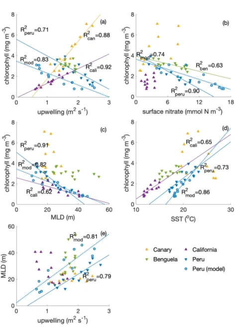
Compared with other EBUS, the Peruvian system is unique in that it shows a clear anti-correlation between surface chlorophyll concentration and upwelling intensity on a seasonal scale, with lowest chlorophyll concentrations when upwelling is most 125
intense (Fig. 2a,R2= 0.71; Chavez and Messié, 2009). While the surface chlorophyll in the Benguela system does not feature a strong seasonality, surface chlorophyll follows upwelling intensity closely in the California (R2= 0.92) and Canary (R2= 0.88) systems, suggesting that upwelling of nutrient-rich waters fuels the chlorophyll increase in these two systems.
Indeed, comparatively low surface nitrate concentrations indicate that nitrate is used up and potentially limiting phytoplank- ton growth throughout the year in the California system, and for about half the year in the Canary system (Fig. 2b). For the 130
remainder of the year, in the Canary system enhanced surface nitrate concentrations are positively correlated with chlorophyll, suggesting that phytoplankton is stimulated by enhanced nitrate availability. In contrast, the Benguela (R2= 0.63) and the Peruvian system (R2= 0.90) feature replete surface nitrate over most of the year. With higher nitrate concentrations correlated with lower chlorophyll, this suggests that nitrate is not limiting.
In the Peruvian system, a strong relationship exists between deepening mixed layers and decreasing chlorophyll (Fig. 2c, 135
R2= 0.91), supportive of the notion that dilution of phytoplankton over a deeper mixed layer and/or light limitation plays a role, as suggested by Echevin et al. (2008). The California system shows a similar albeit damped response to mixed layers variations (R2= 0.62), suggesting that the same process may play a role here, too. The weaker increase of phytoplankton concentrations with shallowing mixed layers compared to the Peruvian system is consistent with a greater role of nutrient limitation. The Benguela system, if at all (insignificant), shows a very weak response to mixed layer depth variations, despite 140
quite some range of mixed layer depths over the course of the year. The Canary system does not feature a substantial mixed layer depth variability. Rather, in the Canary system, mixed layers are shallow throughout the year, possibly contributing with favorable light conditions to comparatively high chlorophyll concentrations throughout the year. All in all, the Peruvian system shows the strongest response to MLD variations.
Surface chlorophyll correlates positively with SST in the Peruvian (Fig. 2d,R2= 0.73) and California systems (R2= 0.65) 145
and to a lesser extent in the Benguela upwelling (R2= 0.41), suggesting that increasing temperatures are stimulating phyto- plankton growth. The Benguela system also upholds the trend of increasing chlorophyll following the increasing temperature, though the correlation is not significant. As for MLD, the Canary system does not reveal a strong seasonal SST variance albeit features comparatively high SSTs throughout the year.
Strikingly, the Peruvian system is the only one of the four EBUS where high upwelling coincides with deep MLD (Fig. 2e, 150
R2= 0.79). The Canary system features a seasonality of upwelling but shallow mixed layers throughout the year, while the Benguela system does not vary much in terms of upwelling while varying in terms of mixed layer depth. In the California system, the relationship of upwelling and mixed layer depth is opposite to that of the Peruvian system, with the highest upwelling into the shallowest mixed layers.
Given the paradox that strong upwelling in the Peruvian system occurs at the time of the yearly chlorophyll minimum, it is 155
intuitive that the concurrent deep mixed layers offset the positive impact of upwelled nutrients. In other words, more nutrients only have a strong local positive effect if concentrations are low / would be low otherwise. If concentrations are elevated, adding more nutrients will have a weak impact. We will look further into the interplay of the seasonality of mixed layers and upwelling in the Peruvian system in the following.
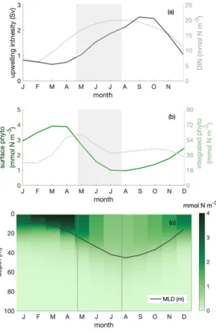
3.2 Modelled phytoplankton biomass, dissolved inorganic nitrogen, upwelling and the MLD in the Peruvian system 160
We use a regional ocean circulation model coupled to a marine biogeochemical model (CROCO-BioEBUS) to further analyse the Peruvian system (see Methods). The model reproduces well the observed estimate of the seasonal out-of-phase relationship of surface phytoplankton biomass with upwelling intensity and nitrate concentrations (Fig. 2, open circles). In the model, surface chlorophyll and nitrogen concentrations together with upwelling intensity and MLD all display a 40-60% seasonal variability. Surface phytoplankton biomass concentration is highest in late austral summer to early autumn (March to April) 165
when upwelling is relatively weak (Fig. 3a,b). Less nitrogen is available within a shallow MLD compared with the rest of the year. In austral winter (July to September), when upwelling brings up ample nitrogen into the deep mixed layer, surface phytoplankton concentration is lowest.
3.3 Biomass dilution by the deepening mixed layer
Dilution of phytoplankton in deepening winter mixed layers is a key driver behind the seasonality of surface phytoplankton 170
concentration. Within the research area, the MLD shows a seasonal variation with the shallowest mixed layer in austral summer (around 10 m), and the deepest mixed layer in austral winter (around 45 m). Phytoplankton is vertically well mixed within the mixed layer throughout the year (Fig. 3c). In austral winter, in the ‘deep-mixing’ regime, phytoplankton is evenly distributed over a relatively deep mixed layer, diluting phytoplankton biomass. Accordingly, phytoplankton biomass concentrations in the mixed layer, and along with it at the surface, decrease. Hence, seasonal mixed layer deepening and shoaling alone is an 175
important factor in driving phytoplankton concentrations at the ocean surface as observed for instance based on satellite images.
While dilution causes a decrease of winter surface phytoplankton biomass, it explains only part of the observed biomass decrease: the decline persists, even though attenuated, if we integrate phytoplankton over the mixed layer (Fig. 3b). The phytoplankton concentration at the surface (and within the mixed layer) declines by around 70% while declines by around 30% for MLD-integrated biomass between late April and late July (shaded area in Fig. 3 & 4, hereafter referred to as the 180
decline phase). The decline of surface phytoplankton concentrations can be attributed to the decline due to the increase of the mixed layer volume∆V (dilution effect, see Eq. 5) and a decrease of the biomass∆B within the mixed layer (through local biological and physical processes, see Eq. 5). During the decline phase,∆V contributes slightly more than half to the concentration change while∆Bcontributes slightly less than half. That is, the dilution effect due to the deepening mixed layer in the decline phase amplifies the decline of surface biomass concentrations by about a factor of two. Yet, dilution can not fully 185
explain the low phytoplankton biomass in conditions of ample supply of nitrogen, MLD-integrated biomass still declines by around 35%.
Figure 2.Correlations of surface chlorophyll (SeaWIFS climatology, in mg m−3) with (a) upwelling (estimated based on winds from QuikSCAT, inSv, digitized from Chavez and Messié (2009), calculations see Messié et al. (2009)); (b) surface nitrate concentration (WOA, inmmol N m−3); (c) MLD (ARGO, in m); (d) SST (MODIS, inoC) and (e) correlation of MLD and upwelling transport among four eastern boundary upwelling systems (EBUS); for the Peruvian system we show also the model (CROCO-BioEBUS) results. Lines andR2values are given for correlations withR2>0.5.
Figure 3.Seasonal cycles of (a) upwelling intensity (inSv, solid line) and surface dissolved inorganic nitrogen (DIN) concentration (in mmol N m−3, dotted line); (b) surface (inmmol N m−3, solid line) and mixed layer depth (MLD)-integrated phytoplankton biomass (in mmol N m−2, dotted line); (c) phytoplankton depth-month distribution with the seasonal cycle of MLD (inm, solid line) within the focus region. The shaded area indicates the decline phase of MLD integrated phytoplankton biomass.
3.4 Biological and physical processes change total biomass within the mixed layer 3.4.1 Disentangling physical and biological processes
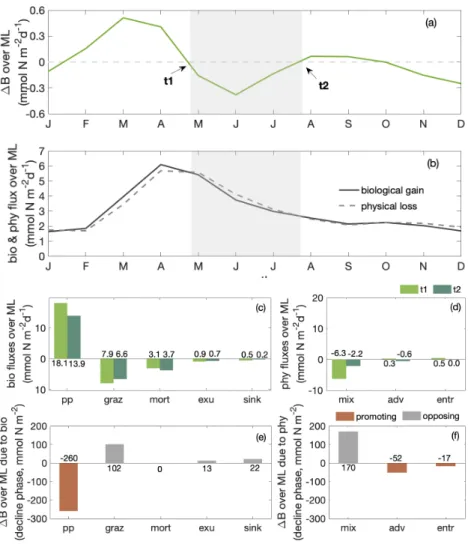
Besides dilution due to the deepening mixed layer, the imbalance of a series of biological and physical processes during the 190
decline phase also diminishes phytoplankton concentrations. To disentangle their contributions to the decline of phytoplankton concentration without the complication of the dilution effect, we next analyze the change of phytoplankton biomass integrated over the mixed layer (Fig. 4a) and its drivers, that is the mixed layer budget of phytoplankton biomass (Eq. 1, Supplementary Fig. C2). We separate biological processes (e.g. primary production, grazing from zooplankton, natural mortality, exudation, sinking) and physical processes (mixing, advection and entrainment) that affect the integrated biomass (Fig. 4b). Throughout 195
the year, the net biological flux is positive, acting as a source for MLD-integrate phytoplankton biomass, while the net physical flux is negative, acting as a sink. The balance of these terms determines if the total biomass within the mixed layer decreases or increases. Most biological and physical processes decrease from the start (t1) to the end (t2) of the decline phase (Fig. 4c- d). While mortality is larger at t2 than t1, it is only due to a sudden increase by the end of the decline phase (Fig.C2). The more rapid decrease of net biological source relative to net physical loss leads to biomass reduction during the decline phase 200
(Fig. 4b).
The biological and physical processes that promote a decline of the MLD-integrated biomass are a reduction of primary production and entrained phytoplankton, along with an enhanced phytoplankton offshore transport (Fig. 4e-f). Among the bi- ological processes, the reduction of primary production as the only source process overpowers the weakening of biological sink processes and significantly promotes the biomass decline. Within the physical processes, the net effect of lateral and ver- 205
tical transport of phytoplankton biomass (advection) is picking up during the decline phase, leading to a net offshore export of phytoplankton biomass. In addition, while phytoplankton is entrained into the mixed layer from below when mixed layers deepen, the rate of entrainment decreases during the decline phase. The decreasing rate is due to decreasing phytoplankton concentrations at the bottom of mixed layers as mixed layers deepen. All other biological and physical processes act to oppose the decline of phytoplankton biomass, such as an attenuation of mixing out of the mixed layer over the decline phase. Details 210
regarding the two major contributors, primary production and advection, are presented in the following sections.
3.4.2 Factors limiting primary production
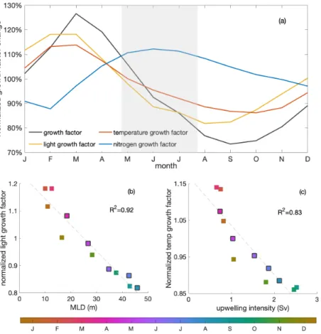
Primary production changes due to variations of both the growth factor and the biomass (Eq. 2). The growth factor (calculated as in Eq. 3, Fig. 5a) combines the effects of light, temperature and nitrogen on phytoplankton growth. It shows a clear decrease 215
(around 30%) during the decline phase. Optimal phytoplankton growth conditions are reached in March despite the low dis- solved inorganic nitrogen (DIN) conditions, with the warmest and brightest environment. The lowest growth rate occurs just after the decline phase despite relatively high nitrogen concentrations due to limiting light and temperature conditions.
Strong light limitation experienced by phytoplankton in combination with low temperatures slows down the growth during the decline phase. Light conditions for phytoplankton growth are best in March when the water is rather stratified and worsens 220
over the decline phase to a minimum in August when the water column is mixed deepest. The light-related growth factor declines by 17% during the decline phase and would decrease the growth factor by around 60% in the absence of other limiting factors (estimated based on Eq. 3). The decreasing temperature is the second most important factor to slow the growth rate in the decline phase. The temperature-related growth factor reaches its maximum by March, similarly to the light-related growth factor, and its minimum by October. The temperature-related growth factor declines by 12% and would decrease the growth 225
factor by around 40% in the absence of other limiting factors during the decline phase. In contrast, the seasonality of the growth factor due to nitrogen shows the opposite seasonality compared to the total growth factor. Clearly, light and temperature regulate primary production and override the effect of nitrogen supply during the decline phase. Therefore, while light is the dominant mechanism that reduces productivity towards winter, we find that temperature plays a relevant secondary role.
Figure 4.Seasonal cycles of (a) total phytoplankton biomass change∆B in the mixed layer (inmmol N m−2d−1); gray shading indicates the decline phase as in Fig. 3, witht1andt2marking the beginning and end of the decline phase; (b) MLD-integrated phytoplankton net biological and physical fluxes (inmmol N m−2d−1, as shown in Eq. 1 plus the entrainment introduced by the integration); bar plots of (c) biological and (d) physical fluxes at the start (t1, light green) and end (t2, dark green) of decline phase; bar plots of the integrated change over the decline phase over mixed layer due to (e) biology and (f) physics within the focus region. Red and grey indicate promoting and opposing ML-integrated phytoplankton biomass decline. pp stands for primary production; graz for consumptive mortality; mort for natural mortality;
exu for exudation; sink for sinking; mix for mixing; adv for advection and entr for entrainment.
Stronger light and temperature limitation during the decline phase are due to deeper mixing and stronger upwelling, respec- 230
tively (Fig. 5b-c). While upwelling intensity is approximately correlated with deep mixed layers occurring when upwelling is high, the peak of upwelling happens just after the deepest mixed layers. The variation of MLD-averaged light limitation is correlated (R2= 0.92) with the change of MLD. As phytoplankton is evenly distributed within the mixed layer, deeper MLD means more phytoplankton is exposed to a relatively lower light condition on average in the decline phase, with a minimum in
Figure 5.(a) Seasonal cycles of the normalized total (black) growth factor, light (yellow)-, temperature (red)- and nitrogen (blue)-related growth factors, as experienced by phytoplankton over the mixed layer. The grey shading indicates the decline phase; (b) seasonal correlation of MLD and mixed layer averaged light-related growth factor; (c) correlation of upwelling intensity and mixed layer averaged temperature- related growth factor. Colors indicate the time of the year (months) with black edges marking the months of the decline phase.R2value of the correlation is shown in the right of the panels
August when mixed layers are deepest. The change of the temperature-related growth factor within the mixed layer is closely 235
related (R2= 0.83) with the seasonal variation of upwelling intensity, with the lowest values in September and October when upwelling intensity is highest. In the decline phase, cold waters are upwelled into the mixed layer at a higher rate, further damping phytoplankton growth in addition to the limiting light conditions. Reduced winter surface solar radiation and heat loss to the atmosphere, also play a role in the seasonality of the light and temperature growth factors, respectively (Fig. C3), yet of much less importance (not shown).
240
3.4.3 Enhanced upwelling and offshore transport of phytoplankton
An enhanced advective loss of mixed layer phytoplankton is a second-order process promoting the decrease of MLD-integrated phytoplankton biomass during the decline phase. Like nutrients, phytoplankton biomass is affected by the seasonality of up- welling and offshore export of waters. Phytoplankton growing at the bottom of the mixed layer is being upwelled and later pushed offshore along with the phytoplankton that is growing in the mixed layer. During the decline phase, the upwelling 245
and offshore transport of water increases and more of what is produced in coastal waters is exported offshore: 4% of primary production is lost via advection by the end of the decline phase compared to 2% gained at the beginning. This greater loss of biomass due to divergent advection is mainly caused by stronger upwelling in the decline phase (Fig. C4).
4 Discussion
4.1 Mixed layer depth drives surface phytoplankton biomass seasonality in the Peruvian upwelling system 250
The regional ocean circulation-biogeochemical model that we use successfully reproduces the "seasonal paradox", with sea- sonal out-of-phase surface chlorophyll concentration and upwelling intensity, as derived from observations. As shown in the results, the low surface chlorophyll concentration in high upwelling conditions in austral winter is constrained by a combined effect of MLD-driven processes and upwelling-driven processes. Under high upwelling conditions in austral winter, phyto- plankton is diluted over a deeper mixed layer, leading to a decrease of the mixed layer, and likewise, surface phytoplankton 255
concentrations by over 50%. Also, phytoplankton growth is slowed down as they experience deteriorating light and temperature conditions. On top of that, strong upwelling pushes phytoplankton offshore.
Several previous studies have also focused on the possible reasons behind the seasonal paradox in the PUS. Echevin et al.
(2008) also suggested based on model results that relative low surface chlorophyll concentration in austral winter off the Pe- ruvian coast is generated by the combined effect of dilution and deteriorating light limitation with deepening mixed layers.
260
In addition, Messié and Chavez (2015) find that more severe iron limitation under low light condition could also be one of the reasons behind low primary production under high upwelling conditions. According to results from culture experiments, phytoplankton iron demand would increase under light limitation conditions (Sunda and Huntsman, 1997). Based on observa- tions, Friederich et al. (2008) suggest that winds in the winter high-upwelling conditions favor curl driven upwelling, which would draw more offshore iron-deficient waters to the surface. On the contrary, a model study (Albert et al., 2010) finds that 265
stronger wind-curl driven upwelling actually is recruiting more nutrient-rich water from a shoaling coastal undercurrent, thus contributing to enhancing surface chlorophyll concentrations. We cannot assess the role of iron in regulating the seasonality of phytoplankton biomass because our biogeochemical model does not simulate iron (see Sect.B). Nevertheless, our study confirms the importance of vertical redistribution of biomass and light limitation due to vertical mixing. Here, we emphasize the importance of the deepening mixed layers in the decline phase.
270
4.2 Upwelling into deep mixed layers: A unique feature of the Peruvian upwelling system and its implications As we just argued in the previous paragraphs using the differences of the seasonalities of MLD and upwelling in the Peruvian system. The upwelling of nutrient rich waters happens when growth conditions are the worst, i.e. light availability is lowest due to deep mixed layers. Also, the upwelled waters are comparatively cool and in deep mixed layers may warm up relatively slowly. At the same time, the upwelling will charge the deep mixed layers with nutrients that allow for growth once the mixed 275
layer shallows. That is, the upwelling into deep mixed layers in the Peruvian may precondition high summer phytoplankton production.
In contrast, in the California system nutrients are upwelled into the shallowest mixed layers. While this nutrient supply coincides with shoaling mixed layers and associated improved light conditions and reduced dilution, it does not result in as high phytoplankton concentrations as for the Peruvian system. This supports that nutrient limitation is important, as the supply 280
of nutrients to shallow mixed layers by upwelling appears insufficient to relieve nutrient limitation. We speculate that the charging of deep mixed layers as in the Peruvian system is more efficient in supplying nutrients to the euphotic zone compared to upwelling into shallow waters as in the Californian system, possibly warranting further studies. Also, if nutrients are being upwelled into deep mixed layers and allow the onset of a bloom, zooplankton standing stock might be low and take a while to catch up and eventually reduce phytoplankton biomass. On the contrary, if nutrients are being upwelled into shallow mixed 285
layers, zooplankton standing stock is probably already high and zooplankton can act on the spot to limit phytoplankton biomass.
While the Canary and Benguela systems lack a seasonality in MLD and phytoplankton, respectively, we mark a few aspects that may point towards a role of MLD also in these systems. Given that the Canary system does not feature a substantial seasonal MLD variability, it is intuitive that it follows the seasonality of upwelling intensity more strongly compared to the other EBUS.
While mixed layer conditions do not modulate the seasonality of phytoplankton they may contribute to Canary high phyto- 290
plankton concentrations insofar as mixed layers are shallow throughout the year, creating favorable light conditions. Finally, the Benguela system features a rather constant upwelling through the year into varying mixed layers. The non-responsiveness of phytoplankton to the varying MLD hypothetically could be due to compensating effects of deepening mixed layers that dilute phytoplankton and deteriorate light conditions, but the same time are accompanied by enhanced supply of nutrients that are mixed up from below. The higher surface nitrate concentrations in conditions of deep mixed layers in the Benguela system 295
could be interpreted this way. Enhanced growth due to higher nutrient availability would then offset, yet not completely, the worsening light conditions and dilution. Finally, the strong response of phytoplankton in the Peruvian upwelling system to mixed layer depth would then be due to the unique situation of upwelling into deep mixed layers.
Again, other factors may also play a role in regulating phytoplankton in the EBUS next to nutrients, dilution and light associated with upwelling and MLD (see also Results section; Messié and Chavez, 2015), including the advection of biomass 300
and regulation by temperature that varies with upwelling (see Results). In addition, Lachkar and Gruber (2011) suggest that a longer residence time because of a wide shelf and weak mesoscale activity may also promote phytoplankton growing. Also, next to iron supply from the shelves and upwelling of source waters, Fung et al. (2000) found that atmospheric deposition of iron varies between EBUS.
4.3 From phytoplankton to ecosystem functioning 305
The interplay of mixed layer depth and upwelling that leads to the seasonal paradox in the PUS is further propagating up the food chain and modulates the trophodynamics. In austral summer, when the shallow mixed layer along with the add- on effect from upwelling supports the highest phytoplankton biomass and primary production, it provides an ideal feeding place for zooplankton. In contrast, in winter zooplankton is facing a food shortage, less efficient grazing due to dilution and transports due to enhanced upwelling. Similar to the spatial match-mismatch observed for phytoplankton and top predator in 310
Benguela system(Grémillet et al., 2008), mesozooplankton with its slower growth rate may also be affected by upwelling, with phytoplankton thriving near the coast and zooplankton concentrated further offshore. In our model, mesozooplankton is responsible for the major part of the export in the coastal upwelling region. During the productive season, the faecal material of mesozooplankton accounts for close to 100% of the sinking matter which is in good agreement with what is found in Stukel et al. (2013) for the California system.
315
Both primary production and export are found to be determined by the mixed layer dynamics and foodweb structures (Ducklow et al., 2001; Turner, 2015; Steinberg and Landry, 2017). The efficiency of the export, defined as the ratio of export to primary production, is also related to trophodynamics. Export efficiency depends, as mentioned above, on the composition of the exported material. In the PUS, it is positively correlated with net primary production (Fig. C5). Mesozooplankton produces fast-sinking large detritus, which enhances the export efficiency during the productive season. In both the Peruvian and Cali- 320
fornia systems, high primary productivity coincides with a shallow MLD. What is different in the California system compared to the Peruvian system is that in the former the time of shallow mixed layers and high primary productivity is also the time of strongest upwelling. Strong upwelling and offshore transport may lead to the above mentioned spatial mismatch between phytoplankton and mesozooplankton, because mesozooplankton grows more slowly. This may then result in comparatively low large detritus despite high primary production. Therefore, high primary production may not necessarily tie in with high 325
mesozooplankton biomass and subsequent high export. Indeed, Kelly et al. (2018) observed that export efficiency is negatively correlated with net primary productivity in the California system. However, they suggested that this negative correlation arises from a seasonal decoupling of export and particle production through long-lived, slowly sinking particles that would introduce a temporal lag of mesozooplankton production and export to depth. In addition, Henson et al. (2019) find a negative correlation between export efficiency and primary productivity on a global scale. They imply in their study that it is not just the phyto- 330
plankton community but also the foodweb structure important to export efficiency. We suggest that the role of the interplay of the mixed layer and upwelling in EBUS and ecosystem functioning is closely linked and warrants further examination.
4.4 Potential change under global warming
Our findings suggest that for an assessment of the response of the EBUS to climate change, it is important to consider the po- tential change of the interplay between the mixed layers and upwelling dynamics. Phytoplankton will inevitably be influenced 335
by climate change, responding to the changes in the biotic and abiotic environment. Impacts in a changing climate will arise from changes of stratification and upwelling that further lead to shifting growth conditions due to changes of light, temperature
and nutrient (Behrenfeld, 2014). Previous observations indicate that waters near the coast have cooled since the 1950s, possi- bly due to an increase in upwelling (Gutiérrez et al., 2011). A recent regional modelling study (Echevin et al., 2020) projects an intensive surface warming along with a weakening of wind-driven upwelling. While studies typically focus on changes in 340
upwelling, our results suggest that MLD changes maybe even more relevant. Assuming that winds will never cease entirely and hence there will always be some upwelling that recharges the mixed layer with nutrients, shoaling of the mixed layer caused by intensive surface warming may dominate the response of phytoplankton and ecosystem functioning. A shoaling MLD may release the phytoplankton from the strong dilution and light limitation in austral winter, along with better light and temperature condition in austral summer, leading to the expectation of an attenuation of the seasonal paradox in future. While modulation 345
of growth conditions due to changing temperatures and nutrient supply from changing upwelling also may play a role, Echevin et al. (2020) simulations suggest that surface chlorophyll overall will increase in the PUS due to global warming.
5 Conclusions
In summary, CROCO-BioEBUS performs well compared to observational data and successfully reproduces the "seasonal paradox" with an out-of-phase relationship of surface chlorophyll and upwelling intensity in the Peruvian coastal waters. The 350
seasonal cycle of surface chlorophyll concentration in our simulations is driven mostly by MLD-related processes (dilution and light limitation), with secondary contributions from upwelling-related processes (temperature limitation and advection). Unlike other EBUS, the PUS features a unique positive correlation of the mixed layer and upwelling, with the strongest upwelling into the deepest mixed layers, whose combined impacts lead to the seasonal fluctuation of surface chlorophyll concentration.
We find that the seasonal variability of phytoplankton further propagates up the food chain and affects the trophodynamics, 355
and ultimately export efficiency. Therefore, a more thorough understanding of the interactions behind the mixed layer and upwelling dynamics along with the food web processes will help to better project how coastal upwelling ecosystems, and in particular the Peruvian system, may vary under climate change.
Code availability. CROCO and BioEBUs models are available at http://www.croco-ocean.org
Data availability. The model data used in this paper are available via the corresponding author 360
Appendix A: Methods
A1 Two-way nesting approach
Figure A1 visualizes the coarser-resolution parent and nested finer-resolution child domain that contains the focus region. The variables in section B are shown for the child domain.
parent child
Figure A1.Bathymetry of the "parent" (1/4◦resolution) and "child" (1/12◦resolution) domains. White lines near the coast highlight the focus region.
A2 Adjustment of biogeochemical model parameters 365
The parameter setting is the same as in José et al. (2017), with only a few biological parameters adjusted to make the ecol- ogy (phyto- and zooplankton biomasses, productivity) better fit observational data. The changed parameters along with value ranges from literature are listed in Table A1 and will be further explained below.
Here, we assign a higher mortality rate for large phytoplankton to simulate the potential impact of virus infection during bloom conditions (Suttle, 2005). Simulated phytoplankton biomass and its seasonality has been calibrated and evaluated against 370
chlorophyll concentration data from MODIS monthly climatology data (https://oceancolor.gsfc.nasa.gov/). Nitrate has been evaluated based on WOA and cruise data while simulated MLD has been validated against the ARGO mixed layer database (Holte et al. (2017), http://mixedlayer.ucsd.edu/).
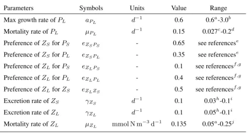
Table A1.Adjusted biological Parameters and range of published parameter values
Parameters Symbols Units Value Range
Max growth rate ofPL aPL d−1 0.6 0.6a-3.0b
Mortality rate ofPL µPL d−1 0.15 0.027c-0.2d
Preference ofZSforPS eZSPS - 0.65 see referencese Preference ofZSforPL eZSPL - 0.35 see referencese Preference ofZLforPS eZLPS - 0.1 see referencesf,g Preference ofZLforPL eZLPL - 0.4 see referencesf,g Preference ofZLforZS eZLZS - 0.5 see referencesf,g
Excretion rate ofZS γZS d−1 0.1 0.03h-0.1i
Excretion rate ofZL γZL d−1 0.1 0.05h-0.1i
Mortality rate ofZL µZL mmol N m−3d−1 0.135 0.05a-0.25j
aGutknecht et al. (2013)
bAndersen et al. (1987)
cKoné et al. (2005)
dTaylor et al. (1991)
eBohata (2016)
fKleppel (1993)
gSchukat et al. (2014)
hAumont (2005)
iFennel et al. (2006)
jLima and Doney (2004)
Appendix B: Model evaluation 375
B1 Surface chlorophyll concentration
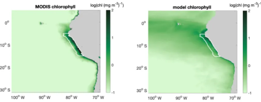
The large-scale spatial pattern of annual average surface chlorophyll of the monthly climatology of MODIS data and CROCO- BioEBUS are similar (Fig. B1), with higher chlorophyll concentrations in coastal regions and lower concentrations offshore (note that chlorophyll is shown in log-scale). The satellite data features a higher cross-shore chlorophyll concentration gradient compared to the model simulation. The model’s overestimation of the low offshore chlorophyll and hence weaker cross-shore 380
gradient potentially is due to the lack of iron limitation in the model. Apart from that, the model is also not able to correctly capture the alongshore pattern (Fig. B1), i.e. it misses two observed high surface chlorophyll concentration patches between 8◦S to 10◦S and 12◦S to 14◦S (Bruland et al., 2005). Within a 200 km band near the coast, both satellite data and the model simulation show a similar seasonality with maximum chlorophyll concentrations exceeding 4 mg /m3from March to April and minimum concentrations around 2 mg /m3in August. In general, simulated surface chlorophyll concentrations agree reasonably 385
well with satellite data.
Figure B1.Annual mean surface chlorophyll concentration (inlog(chl (mg m−3)−1)) distribution of (a) MODIS and (b) CROCO-BioEBUS.
White lines highlight the focus region.
B2 Surface nitrate concentration
The simulated surface nitrate distribution shows the same seasonality as observations from the World Ocean Atlas (WOA;
Garcia et al., 2019) (Fig. B2). The simulated surface nitrate concentration in the coastal region is biased high compared to the 390
WOA data. This may be partly due to the WOA data failing to capture high-nitrate concentrations due to coastal upwelling.
This notion is supported by nitrate concentration data from a cruise in austral summer that show nitrate concentrations in the coastal region are high compared to the model data.
B3 Mixed layer depth
We validate the simulated MLD against the gridded ARGO mixed layer dataset (Holte et al. (2017), http://mixedlayer.ucsd.edu/) 395
both in terms of spatial pattern and seasonal variability within the research area (Fig. B3). The annually averaged spatial dis- tribution of MLD within the research area presents the same features as ARGO: shallower MLD in the coastal region (around 20 m) and deeper MLD in the offshore region (around 80 m). The simulated seasonal variability of MLD within the research region generally follows the seasonal trend of the Argo data. The water column within the research region is most stratified in February to March and most deeply mixed in August. Although simulated MLD in austral winter is somewhat deep, the 400
simulated MLD are largely within the range of the ARGO data.
B4 Sea surface temperature
The simulated SST has been validated against monthly climatological MODIS data in terms of both spatial pattern and seasonal variability within the research area (Fig. B4). The annually averaged spatial distribution of SST is well simulated by the model.
The model successfully captures the cold coastal upwelled water as well as slightly warmer water masses further offshore.
405
The simulated SST seasonality within the research region generally follows the seasonal trend of the observations, with a cool bias of less than 1oC. The surface waters within the research region are warmest in February to March matching the
Figure B2.Spatial distribution of surface nitrate concentration based on (a) WOA and (b) CROCO-BioEBUS; (c) January and (d) February as simulated by CROCO-BioEBUS. Dots indicate measurements from the cruises M92 (January) and M93 (February); (e) seasonal cycle of surface nitrate concentration from WOA (cross), CROCO-BioEBUS (line) and cruises (pentagram, hexagram) within the focus region.
White lines highlight the focus region. The black box indicates the maps of panel c-d.
modelled/observed shallowest mixed layers and coldest from August to October. In general, the simulated SST matches the observations well both in terms of spatial pattern and seasonal variation.
Figure B3.Annual average spatial distribution of mixed layer depth (MLD) from (a) ARGO and (b) CROCO-BioEBUS; (c) Seasonal variation of average mixed layer depth from ARGO (crosses, with lines indicating the standard deviation) and model simulation (line) within focus region. White lines highlight the focus region.
Appendix C: Additional Figures 410
The whole time series of temperature and nitrate concentration at 10 m and 1000 m are shown in Fig. C1a-b. Surface fields are spun up after one year while deepwater takes longer to reach a steady state. In the meanwhile, mixed layer and surface layer chlorophyll are also spun up after one year (Fig. C1c-d).
Detailed seasonal cycles of phytoplankton budgets integrated over MLD is shown in Fig.C2, including primary production (pp), consumptive mortality (graz), natural mortality (mort), exudation (exu), sinking (sink), mixing (mix), advection (adv) 415
and entrainment (entr). Further, seasonalities of net biological (bio) and physical (phy) fluxes along with MLD-integrated phytoplankton biomass change (∆B) is also shown in the figure.
Apart from above mentioned mixed layer depth and upwelling intensity, short-wave surface radiation and surface net heat flux are of second-order importance to light- and temperature-related variance during the decline phase respectively (Fig.C3).
Phytoplankton net advection flux over the mixed layer closely follows the upwelling intensity during the decline phase 420
(Fig.C4,R2= 0.81). When the mixed layer depth is relatively shallow, the correlation between upwelling intensity and phyto- plankton convergence of advection over the mixed layer is insignificant.
Figure B4.Annual average spatial distribution of sea surface temperature (SST, inoC) from (a) MODIS and (b) CROCO-BioEBUS; (c) Seasonal variation of average sea surface temperature (SST) from MODIS (cross) and model simulation (line) within focus region. White lines highlight the focus region.
We define export as the organic material sinking below the euphotic layer and export efficiency as the ratio of primary production over export (Murray et al., 1996). The efficiency of export depends on the composition of particle organic matter with different sinking speed and its remineralization rate. Within the model, export efficiency is positively correlated with net 425
primary production (Fig.C5) which is opposite to what is found in the California system.
Figure C1.Time series of temperature T (at 10 m & 1000 m depth), nitrate N (at 10 m & 1000 m depth), mixed layer depth MLD and phytoplankton phyto (at 10 m) over 30 years of simulation in the focus region.
Figure C2.Seasonal cycles of phytoplankton source and sink processes integrated over the mixed layer, along with the net biological fluxes (dotted line) and the net physical fluxes (dashed line), and the tendency (change) of phytoplankton biomass (solid line) integrated over the mixed layer.
Figure C3.(a) Correlation between surface short-wave radiation (Wm−2) and the averaged light-related growth factor within mixed layer;
(b) Correlation between the surface heat forcing (inoCd−1) and averaged temperature-related growth factor within mixed layer. Color indicates the time of the year and black edges the decline phase.
Figure C4.Correlation between upwelling intensity and phytoplankton convergence of advection over the mixed layer. A negative conver- gence equals a divergence of phytoplankton biomass due to the combined effect of upwelling and lateral transports. Color indicates the time of the year and black edges the decline phase. The correlation coefficient (R2=0.81) is shown for the decline phase.
Figure C5.Correlation of export efficiency (defined as ratio of primary production over export below the euphotic layer) with net primary production (NPP). Colors indicate the time of the year.
Author contributions. IF and AO designed the study. TX and YSJ carried out the simulations. TX, IF and FP conducted the analysis. All authors discussed the results and wrote the manuscript.
Competing interests. The authors declare that they have no conflict of interest.
Acknowledgements. This work is financially supported by the China Scholarship Council (TX, grant no.201808460055). Further support 430
for this work was provided by the BMBF funded projects Coastal Upwelling System in a Changing Ocean CUSCO (IF, AO) and Humboldt Tipping (YJ).
References
Albert, A., Echevin, V., Lévy, M., and Aumont, O.: Impact of nearshore wind stress curl on coastal circulation and primary productivity in the Peru upwelling system, Journal of Geophysical Research: Oceans, 115, 2010.
435
Andersen, V., Nival, P., and Harris, R. P.: Modelling of a planktonic ecosystem in an enclosed water column, Journal of the Marine Biological Association of the United Kingdom, 67, 407–430, 1987.
Aumont, O.: PISCES biogeochemical model, Unpublished report, 2005.
Bakun, A.: Coastal upwelling indices, west coast of North America, 1946-71, 1973.
Bakun, A.: Global climate change and intensification of coastal ocean upwelling, Science, 247, 198–201, 1990.
440
Bakun, A., Field, D. B., Redondo-Rodriguez, A., and Weeks, S. J.: Greenhouse gas, upwelling-favorable winds, and the future of coastal ocean upwelling ecosystems, Global Change Biology, 16, 1213–1228, 2010.
Behrenfeld, M. J.: Climate-mediated dance of the plankton, Nature Climate Change, 4, 880–887, 2014.
Bohata, K.: Microzooplankton of the northern Benguela Upwelling System, PhD thesis, 2016.
Bruland, K. W., Rue, E. L., Smith, G. J., and DiTullio, G. R.: Iron, macronutrients and diatom blooms in the Peru upwelling regime: brown 445
and blue waters of Peru, Marine Chemistry, 93, 81–103, 2005.
Calienes, R., Guillén, O., Lostaunau, N., et al.: Variabilidad espacio-temporal de clorofila, producción primaria y nutrientes frente a la costa peruana, Boletin Instituto del Mar del Peru, 10, 1–44, 1985.
Carton, J. A. and Giese, B. S.: A reanalysis of ocean climate using Simple Ocean Data Assimilation (SODA), Monthly Weather Review, 136, 2999–3017, 2008.
450
Chavez, F. P. and Messié, M.: A comparison of eastern boundary upwelling ecosystems, Progress in Oceanography, 83, 80–96, 2009.
Chavez, F. P., Bertrand, A., Guevara-Carrasco, R., Soler, P., and Csirke, J.: The northern Humboldt Current System: Brief history, present status and a view towards the future, Progress in Oceanography, 79, 95–105, 2008.
Debreu, L., Marchesiello, P., Penven, P., and Cambon, G.: Two-way nesting in split-explicit ocean models: Algorithms, implementation and validation, Ocean Modelling, 49, 1–21, 2012.
455
Ducklow, H. W., Steinberg, D. K., and Buesseler, K. O.: Upper ocean carbon export and the biological pump, OCEANOGRAPHY- WASHINGTON DC-OCEANOGRAPHY SOCIETY-, 14, 50–58, 2001.
Echevin, V., Aumont, O., Ledesma, J., and Flores, G.: The seasonal cycle of surface chlorophyll in the Peruvian upwelling system: A modelling study, Progress in Oceanography, 79, 167–176, 2008.
Echevin, V., Gévaudan, M., Espinoza-Morriberón, D., Tam, J., Aumont, O., Gutierrez, D., and Colas, F.: Physical and biogeochemical 460
impacts of RCP8. 5 scenario in the Peru upwelling system, Biogeosciences, 17, 3317–3341, 2020.
Fennel, K., Wilkin, J., Levin, J., Moisan, J., O’Reilly, J., and Haidvogel, D.: Nitrogen cycling in the Middle Atlantic Bight: Results from a three-dimensional model and implications for the North Atlantic nitrogen budget, Global Biogeochemical Cycles, 20, 2006.
Friederich, G. E., Ledesma, J., Ulloa, O., and Chavez, F. P.: Air–sea carbon dioxide fluxes in the coastal southeastern tropical Pacific, Progress in Oceanography, 79, 156–166, 2008.
465
Fuenzalida, R., Schneider, W., Garcés-Vargas, J., Bravo, L., and Lange, C.: Vertical and horizontal extension of the oxygen minimum zone in the eastern South Pacific Ocean, Deep Sea Research Part II: Topical Studies in Oceanography, 56, 992–1003, 2009.
Fung, I. Y., Meyn, S. K., Tegen, I., Doney, S. C., John, J. G., and Bishop, J. K.: Iron supply and demand in the upper ocean, Global Biogeochemical Cycles, 14, 281–295, 2000.
Garcia, H., Weathers, K., Paver, C., Smolyar, I., Boyer, T., Locarnini, M., Zweng, M., Mishonov, A., Baranova, O., Seidov, D., et al.: World 470
Ocean Atlas 2018. Vol. 4: Dissolved Inorganic Nutrients (phosphate, nitrate and nitrate+ nitrite, silicate), 2019.
Getzlaff, J., Dietze, H., and Oschlies, A.: Simulated effects of southern hemispheric wind changes on the Pacific oxygen minimum zone, Geophysical Research Letters, 43, 728–734, 2016.
Grémillet, D., Lewis, S., Drapeau, L., van Der Lingen, C. D., Huggett, J. A., Coetzee, J. C., Verheye, H. M., Daunt, F., Wanless, S., and Ryan, P. G.: Spatial match–mismatch in the Benguela upwelling zone: should we expect chlorophyll and sea-surface temperature to 475
predict marine predator distributions?, Journal of Applied Ecology, 45, 610–621, 2008.
Guillen, O. and Calienes, R.: Upwelling off chimbote, Coastal upwelling, 1, 312–326, 1981.
Gutiérrez, D., Bouloubassi, I., Sifeddine, A., Purca, S., Goubanova, K., Graco, M., Field, D., Méjanelle, L., Velazco, F., Lorre, A., et al.:
Coastal cooling and increased productivity in the main upwelling zone off Peru since the mid-twentieth century, Geophysical Research Letters, 38, 2011.
480
Gutknecht, E., Dadou, I., Le Vu, B., Cambon, G., Sudre, J., Garçon, V., Machu, E., Rixen, T., Kock, A., Flohr, A., et al.: Coupled physi- cal/biogeochemical modeling including O2-dependent processes in the Eastern Boundary Upwelling Systems: application in the Benguela, Biogeosciences, 10, 3559–3591, 2013.
Henson, S., Le Moigne, F., and Giering, S.: Drivers of carbon export efficiency in the global ocean, Global biogeochemical cycles, 33, 891–903, 2019.
485
Holte, J., Talley, L. D., Gilson, J., and Roemmich, D.: An Argo mixed layer climatology and database, Geophysical Research Letters, 44, 5618–5626, 2017.
José, Y. S., Dietze, H., and Oschlies, A.: Linking diverse nutrient patterns to different water masses within anticyclonic eddies in the upwelling system off Peru, Biogeosciences, 14, 1349–1364, 2017.
Kelly, T. B., Goericke, R., Kahru, M., Song, H., and Stukel, M. R.: CCE II: Spatial and interannual variability in export efficiency and the bio- 490
logical pump in an eastern boundary current upwelling system with substantial lateral advection, Deep Sea Research Part I: Oceanographic Research Papers, 140, 14–25, 2018.
Kleppel, G.: On the diets of calanoid copepods, Marine Ecology-Progress Series, 99, 183–183, 1993.
Koné, n. V., Machu, E., Penven, P., Andersen, V., Garçon, V., Fréon, P., and Demarcq, H.: Modeling the primary and secondary productions of the southern Benguela upwelling system: A comparative study through two biogeochemical models, Global Biogeochemical Cycles, 495
19, 2005.
Lachkar, Z. and Gruber, N.: What controls biological production in coastal upwelling systems? Insights from a comparative modeling study, Biogeosciences, 8, 2961–2976, 2011.
Lima, I. D. and Doney, S. C.: A three-dimensional, multinutrient, and size-structured ecosystem model for the North Atlantic, Global Biogeochemical Cycles, 18, 2004.
500
Liu, W. T., Tang, W., and Polito, P. S.: NASA scatterometer provides global ocean-surface wind fields with more structures than numerical weather prediction, Geophysical Research Letters, 25, 761–764, 1998.
Messié, M. and Chavez, F. P.: Seasonal regulation of primary production in eastern boundary upwelling systems, Progress in Oceanography, 134, 1–18, 2015.
Messié, M., Ledesma, J., Kolber, D. D., Michisaki, R. P., Foley, D. G., and Chavez, F. P.: Potential new production estimates in four eastern 505
boundary upwelling ecosystems, Progress in Oceanography, 83, 151–158, 2009.
Murray, J. W., Young, J., Newton, J., Dunne, J., Chapin, T., Paul, B., and McCarthy, J. J.: Export flux of particulate organic carbon from the central equatorial Pacific determined using a combined drifting trap-234Th approach, Deep Sea Research Part II: Topical Studies in Oceanography, 43, 1095–1132, 1996.
O’Reilly, J. E., Maritorena, S., Mitchell, B. G., Siegel, D. A., Carder, K. L., Garver, S. A., Kahru, M., and McClain, C.: Ocean color 510
chlorophyll algorithms for SeaWiFS, Journal of Geophysical Research: Oceans, 103, 24 937–24 953, 1998.
Pauly, D., Christensen, V., Dalsgaard, J., Froese, R., and Torres, F.: Fishing down marine food webs, Science, 279, 860–863, 1998.
Pennington, J. T., Mahoney, K. L., Kuwahara, V. S., Kolber, D. D., Calienes, R., and Chavez, F. P.: Primary production in the eastern tropical Pacific: A review, Progress in oceanography, 69, 285–317, 2006.
Ridgway, K., Dunn, J., and Wilkin, J.: Ocean interpolation by four-dimensional weighted least squares—Application to the waters around 515
Australasia, Journal of atmospheric and oceanic technology, 19, 1357–1375, 2002.
Schukat, A., Auel, H., Teuber, L., Lahajnar, N., and Hagen, W.: Complex trophic interactions of calanoid copepods in the Benguela upwelling system, Journal of Sea Research, 85, 186–196, 2014.
Shchepetkin, A. F. and McWilliams, J. C.: The regional oceanic modeling system (ROMS): a split-explicit, free-surface, topography- following-coordinate oceanic model, Ocean modelling, 9, 347–404, 2005.
520
Steinberg, D. K. and Landry, M. R.: Zooplankton and the ocean carbon cycle, Annual review of marine science, 9, 413–444, 2017.
Stramma, L., Schmidtko, S., Levin, L. A., and Johnson, G. C.: Ocean oxygen minima expansions and their biological impacts, Deep Sea Research Part I: Oceanographic Research Papers, 57, 587–595, 2010.
Stukel, M. R., Ohman, M. D., Benitez-Nelson, C. R., and Landry, M. R.: Contributions of mesozooplankton to vertical carbon export in a coastal upwelling system, Marine Ecology Progress Series, 491, 47–65, 2013.
525
Sunda, W. G. and Huntsman, S. A.: Interrelated influence of iron, light and cell size on marine phytoplankton growth, Nature, 390, 389–392, 1997.
Suttle, C. A.: Viruses in the sea, Nature, 437, 356–361, 2005.
Taylor, A., Watson, A., Ainsworth, M., Robertson, J., and Turner, D.: A modelling investigation of the role of phytoplankton in the balance of carbon at the surface of the North Atlantic, Global Biogeochemical Cycles, 5, 151–171, 1991.
530
Turner, J. T.: Zooplankton fecal pellets, marine snow, phytodetritus and the ocean’s biological pump, Progress in Oceanography, 130, 205–
248, 2015.
Worley, S. J., Woodruff, S. D., Reynolds, R. W., Lubker, S. J., and Lott, N.: ICOADS release 2.1 data and products, International Journal of Climatology: A Journal of the Royal Meteorological Society, 25, 823–842, 2005.