Biogenic halocarbons from the Peruvian upwelling region as tropospheric halogen source

(1)

www.atmos-chem-phys.net/16/12219/2016/

doi:10.5194/acp-16-12219-2016

Biogenic halocarbons from the Peruvian upwelling region as tropospheric halogen source

Helmke Hepach^1,a, Birgit Quack¹, Susann Tegtmeier¹, Anja Engel¹, Astrid Bracher^2,3, Steffen Fuhlbrügge¹, Luisa Galgani^1,b, Elliot L. Atlas⁴, Johannes Lampel⁵, Udo Frieß⁵, and Kirstin Krüger⁶

1GEOMAR Helmholtz Centre for Ocean Research, Kiel, Germany

2Alfred Wegener Institute (AWI), Helmholtz Centre for Polar and Marine Research, Bremerhaven, Germany

3Institute of Environmental Physics, University of Bremen, Bremen, Germany

4Rosenstiel School of Marine and Atmospheric Science (RSMAS), University of Miami, Miami, USA

5Institute of Environmental Physics, University of Heidelberg, Heidelberg, Germany

6Department of Geosciences, University of Oslo, Oslo, Norway

anow at: Environment Department, University of York, York, UK

bnow at: Department of Biotechnology, Chemistry and Pharmacy, University of Siena, Siena, Italy Correspondence to:Helmke Hepach (hhepach@geomar.de)

Received: 15 January 2016 – Published in Atmos. Chem. Phys. Discuss.: 14 March 2016 Revised: 16 August 2016 – Accepted: 1 September 2016 – Published: 29 September 2016

Abstract.Halocarbons are produced naturally in the oceans by biological and chemical processes. They are emitted from surface seawater into the atmosphere, where they take part in numerous chemical processes such as ozone destruction and the oxidation of mercury and dimethyl sul- fide. Here we present oceanic and atmospheric halocarbon data for the Peruvian upwelling zone obtained during the M91 cruise onboard the research vesselMETEORin Decem- ber 2012. Surface waters during the cruise were characterized by moderate concentrations of bromoform (CHBr₃) and dibromomethane (CH₂Br₂) correlating with diatom biomass derived from marker pigment concentrations, which sug- gests this phytoplankton group is a likely source. Concentra- tions measured for the iodinated compounds methyl iodide (CH₃I) of up to 35.4 pmol L⁻¹, chloroiodomethane (CH₂ClI) of up to 58.1 pmol L⁻¹ and diiodomethane (CH2I2) of up to 32.4 pmol L⁻¹ in water samples were much higher than previously reported for the tropical Atlantic upwelling systems. Iodocarbons also correlated with the diatom biomass and even more significantly with dissolved organic matter (DOM) components measured in the surface water. Our re- sults suggest a biological source of these compounds as a significant driving factor for the observed large iodocarbon concentrations. Elevated atmospheric mixing ratios of CH₃I (up to 3.2 ppt), CH₂ClI (up to 2.5 ppt) and CH₂I₂ (3.3 ppt)

above the upwelling were correlated with seawater concentrations and high sea-to-air fluxes. During the first part of the cruise, the enhanced iodocarbon production in the Peru- vian upwelling contributed significantly to tropospheric iodine levels, while this contribution was considerably smaller during the second part.

1 Introduction

Brominated and iodinated short-lived halocarbons from the oceans contribute to tropospheric and stratospheric chemistry (von Glasow et al., 2004; Saiz-Lopez et al., 2012b; Car- penter and Reimann, 2014). They are significant carriers of iodine and bromine into the marine atmospheric boundary layer (Salawitch, 2006; Jones et al., 2010; Yokouchi et al., 2011; Saiz-Lopez et al., 2012b), where they and their degradation products may also be involved in aerosol and ultra-fine particle formation (O’Dowd et al., 2002; Burkholder et al., 2004). Furthermore, they play an important role for ozone chemistry and other processes such as the oxidation of several atmospheric constituents in the troposphere (Saiz-Lopez et al., 2012a). Numerous modelling studies over the last years have shown that brominated short-lived compounds and their degradation products can be entrained into the stratosphere

(2)

and enhance the halogen-driven ozone destruction (Carpen- ter and Reimann, 2014; Hossaini et al., 2015). Recently, it was suggested that oceanic iodine in organic or inorganic form can also contribute to the stratospheric halogen loading, however only in small amounts due to its strong degradation (Tegtmeier et al., 2013; Saiz-Lopez et al., 2015).

While different source and sink processes determine the distribution of halocarbons in the oceanic surface water, the underlying mechanisms are largely unresolved. Biolog- ical activity plays a role for the production of bromoform (CHBr₃), dibromomethane (CH₂Br₂), methyl iodide (CH₃I), chloroiodomethane (CH2ClI) and diiodomethane (CH2I2) (Gschwend et al., 1985; Tokarczyk and Moore, 1994; Moore et al., 1996), while CH3I also originates from photochemical reactions with dissolved organic matter (DOM) (Moore and Zafiriou, 1994; Bell et al., 2002; Shi et al., 2014).

Biologically mediated halogenation of DOM (Lin and Manley, 2012; Liu et al., 2015) and bromination of compounds such as β-diketones via enzymes like bromoperox- idase (BPO) within or outside the algal cells (Theiler et al., 1978) are among the potentially important production processes of CHBr₃and CH₂Br₂. Air–sea gas exchange into the atmosphere is the most important sink for both compounds in the surface ocean (Quack and Wallace, 2003; Hepach et al., 2015).

The biological formation of CH₃I has been investigated during laboratory and field studies (Scarratt and Moore, 1998; Amachi et al., 2001; Fuse et al., 2003; Smythe-Wright et al., 2006; Brownell et al., 2010; Hughes et al., 2011) iden- tifying phyto- and bacterioplankton as producers, revealing large variability in biological production rates. However, bio- geochemical modelling studies suggest that photochemistry may be more important for global CH₃I production (Stemm- ler et al., 2014). Due to their much shorter lifetime in surface water and the atmosphere, fewer studies have investigated production processes of CH₂I₂and CH₂ClI. CH₂I₂has been suggested to be produced by both phytoplankton (Moore et al., 1996) and bacteria (Fuse et al., 2003; Amachi, 2008).

The main source for CH₂ClI is likely its production during the photolysis of CH₂I₂ with a yield of 35 % based on a laboratory study (Jones and Carpenter, 2005). CH₂ClI has also been detected in phytoplankton cultures (Tokarczyk and Moore, 1994), where it may originate from direct production or also from CH2I2conversion. The main sink for both CH2I2and CH2ClI is photolytical breakdown in the surface ocean resulting in lifetimes of less than 10 min (CH2I2) and 9 h (CH₂ClI), respectively, in the tropical ocean (Jones and Carpenter, 2005; Martino et al., 2006). Other sinks for these three iodocarbons are air–sea gas exchange and chloride sub- stitution. The latter may play an important role for CH₃I in low latitudes at low wind speeds (Zafiriou, 1975; Jones and Carpenter, 2007).

Oceanic measurements of natural halocarbons are sparse (Ziska et al., 2013), but they reveal that especially tropical and subtropical upwelling systems are potentially important

source regions (Quack et al., 2007a; Raimund et al., 2011).

Previously observed high tropospheric iodine monoxide (IO) levels in the tropical eastern Pacific have been related to short-lived iodinated compounds in surface waters (Schön- hardt et al., 2008; Dix et al., 2013). However, iodocarbon fluxes have not been considered high enough to explain observed IO concentrations (Jones et al., 2010; Mahajan et al., 2010; Großmann et al., 2013; Lawler et al., 2014), and re- cent global modelling studies have suggested abiotic sources contributing on average about 75 % to the IO budget (Prados- Roman et al., 2015). Such abiotic sources could be emissions of hypoiodous acid (HOI) and molecular iodine (I2) as recently confirmed by a laboratory study (Carpenter et al., 2013).

This paper characterizes the Peruvian upwelling region between 5.0^◦S, 82.0^◦W and 16.2^◦S, 76.8^◦W with regard to the two brominated compounds CHBr₃and CH₂Br₂ and the iodinated compounds CH₃I, CH₂ClI and CH₂I₂ in water and atmosphere. CH₂ClI and CH₂I₂ were measured for the first time in this region. Possible oceanic sources based on the analysis of phytoplankton species composition and different DOM components were evaluated and identified.

Sea-to-air fluxes of these halogenated compounds were derived and their contribution to the tropospheric iodine loading above the tropical eastern Pacific were estimated by combining halocarbon, IO measurements and model calculations.

2 Methods

The M91 cruise of the R/VMETEORfrom 1 to 26 December 2012 investigated the surface ocean and atmosphere of the Peruvian upwelling region (Bange, 2013). From the northernmost location of the cruise at 5.0^◦S and 82.0^◦W, the ship moved to the southernmost position at 16.2^◦S and 76.8^◦W with several transects perpendicular to the coast, alternating between open-ocean and coastal upwelling (Fig. 1). All underway measurements were taken from a continuously oper- ating pump in the ship’s hydrographic shaft from a depth of 6.8 m. Sea surface temperature (SST) and sea surface salinity (SSS) were measured continuously with a SeaCAT thermos- alinograph from Sea-Bird Electronics (SBE).

Deep samples were taken from 4 to 10 depths between 1 and 2000 m from 12 L Niskin bottles attached to a 24-bottle rosette sampler equipped with a CTD and an oxygen sensor from SBE. Halocarbon samples were collected at 24 of the total 98 casts. The uppermost sample from the depth profiles (between 1 and 10 m) was included in the surface water measurements.

2.1 Analysis of halocarbon samples

Halocarbon samples were taken every 3 h throughout the whole day from sea surface water and air. Water was sam- pled bubble-free in 300 mL amber glass bottles. Surface wa-

(3)

$AYSIN$ECEMBER

334;²#= 333$).$)0

.UTRIENTS;MOL,=

) )) ))) )6

./

0/

3I/

.(

(a)

(b)

²3

²7 ²7 ²7

4#HLA;G,=

#ALLAO )

))

)))

)6

(c)

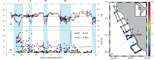
Figure 1.Ambient parameters during the M91 cruise: SST (dark red) and sea surface salinity (SSS) (black) in panel(a)with the dashed line as the mean SST. Nutrients (purple is nitrate – NO⁻₃; yellow is phosphate – PO³⁻₄ ; black is silicate – SiO₂; light cyan is ammonium – NH⁺₄) with the N to P ratio (dark-blue dashed line) are shown in panel(b). Total chlorophylla(TChla) is shown in the map in panel(c). The light-blue shaded areas stand for the regions where SST is below the mean, indicating upwelling of cold water. All M91 data can be accessed at PANGAEA (Hepach et al., 2016).

ter samples were analysed on board with a purge and trap system attached to a GC-MS (combined gas chromatograph and mass spectrometer), which is described in more detail in Hepach et al. (2014). The depth profile samples were analysed with a similar setup: a purge and trap system was attached to a GC equipped with an ECD (electron capture detector). The precision of the measurements was within 10 % for all five halocarbons determined from duplicates and both systems were calibrated using the same liquid stan- dards in methanol. The purge efficiency for all compounds in both setups was larger than 98 % with a sample volume of 50 mL, a purging temperature of 70^◦C, and a purge stream of 30 mL min⁻¹. Halocarbon measurements in seawater started only on 9 December due to instrument issues. Atmospheric halocarbon samples were taken in pre-cleaned stainless steel canisters on the monkey deck at a height of 20 m above sea level using a metal bellows pump starting on 1 December, and were analysed at the Rosenstiel School of Marine and Atmospheric Science (RSMAS) as described in Schauffler et al. (1998). For further details of atmospheric measurements, see Fuhlbrügge et al. (2016a). Quantification was achieved using the NOAA standard SX3573 from GEOMAR.

2.2 Biological parameters

Phytoplankton composition was derived from pigment concentrations. Samples were taken in parallel with the halocarbon samples in the sea surface and up to six samples in depths between 3 and 200 m. Water was filtered through GF/F filters, which were stored at−80^◦C until analysis after shock-freezing in liquid nitrogen. Pigments as described in Taylor et al. (2011) were analysed using a HPLC technique according to Barlow et al. (1997). We used the diagnostic

pigment analysis by Vidussi et al. (2001), subsequently re- fined by Uitz et al. (2006) by introducing pigment specific weight coefficients, to determine the chlorophylla (Chla) concentration of seven groups of phytoplankton which are assumed to comprise the entire phytoplankton community in ocean waters. Identified phytoplankton groups include diatoms, chlorophytes, dinoflagellates, haptophytes, cyanobacteria, cryptophytes and chrysophytes. Total chlorophyll a (TChla) concentrations were calculated from the sum of the pigment concentrations of monovinyl Chla, divinyl Chla and chlorophyllidea.

Samples for the identification of DOM components were taken at 37 stations from a rubber boat from subsurface water at approximately 20 cm. Very well mixed layers at these measurement locations reach down to between 6 and 25 m, and DOM turnover times for the respective compounds has been reported to be several days to months (Engel et al., 2011; Hansell, 2013). All samples were processed onboard and analysed back in the home laboratory. Samples were analysed for dissolved and total organic carbon (DOC and TOC), total dissolved nitrogen (TDN) and total nitrogen (TN) by a high-temperature catalytic oxidation method using a TOC analyser (TOC-VCSH) from Shimadzu. To- tal, dissolved and particulate high-molecular-weight (HMW,

> 1 kDa) combined carbohydrates (TCCHO, DCCHO and PCCHO), as well as total, dissolved and particulate combined HMW uronic acids (TURA, DURA and PURA), i.e.

galacturonic acid and glucuronic acid, were analysed by means of high-performance anion exchange chromatography coupled with pulsed amperometric detection (HPAEC-PAD) after Engel and Händel (2011). For a more detailed descrip-

(4)

tion of both the sampling method and analysis, see Engel and Galgani (2016a), and for data see Hepach et al. (2016).

2.3 Correlation analysis

Correlation analyses between all halocarbons, biological proxies and ambient parameters were carried out using Matlab^® for all collocated surface and depth samples. All datasets were tested for normal distribution using the Lil- liefors test. Since most of the data were not distributed nor- mally, Spearman’s rank correlation (hereinafterrs) was used.

All correlations with a significance level of smaller than 5 % (p< 0.05) were regarded as significant.

2.4 Calculation of sea-to-air fluxes

Sea-to-air fluxes,F, of halocarbons were calculated according to Eq. (1):

F =k_w×

c_w−catm

H

, (1)

wherek_w is the gas exchange coefficient parameterized according to Nightingale et al. (2000),c_wandc_atmare the water concentrations from the halocarbon underway measurements and from the simultaneous atmospheric measurements, respectively, and H is the Henry’s law constant to derive the equilibrium concentration. The gas exchange coefficient usually applied to derive carbon dioxide fluxes was adjusted for halocarbons using Schmidt number corrections as calculated in Quack and Wallace (2003), and Henry’s law coefficients as reported for each of the compounds by Moore et al. (1995) were applied. Wind speed and air pressure were averaged to 10 min intervals for the calculation of the instantaneous fluxes.

2.5 MAX-DOAS measurements of IO

Multi-axis differential optical absorption spectroscopy (MAX-DOAS) (Hönninger, 2002; Platt and Stutz, 2008) observations were conducted continuously in the daytime from 30 November to 25 December 2012 in order to quantify tropospheric abundances of IO, BrO, HCHO, glyoxal, NO₂and HONO along the cruise track, as well as aerosol profiles of O4. The MAX-DOAS instrument and the measurement pro- cedure are described in Großmann et al. (2013) and Lampel et al. (2015).

The primary quantity derived from MAX-DOAS measurements is the differential slant column density (dSCD), which represents the difference in path-integrated concentrations between two measurements in the off-axis and zenith di- rection. From the MAX-DOAS observations of O₄ dSCD aerosol extinction profiles to estimate the quality of visibil- ity were inferred using an optimal estimation approach described in Frieß et al. (2006) and Yilmaz (2012) after apply- ing a correction factor of 1.25 to the O₄dSCDs (Clémer et al., 2010). IO was analysed in the spectral range from 418

to 438 nm following the settings in Lampel et al. (2015). IO was found up to 6 times above the detection limit (twice the measurement error).

2.6 FLEXPART simulations of tropospheric iodine The atmospheric transport of the iodocarbons from the oceanic surface into the marine atmospheric boundary layer (MABL) was simulated with the Lagrangian particle dispersion model FLEXPART (Stohl et al., 2005), which has been used extensively in studies of long-range and mesoscale transport (Stohl and Trickl, 1999). FLEXPART is an off- line model driven by external meteorological fields. It in- cludes parameterizations for moist convection, turbulence in the boundary layer, dry deposition, scavenging, and the sim- ulation of chemical decay. We simulate trajectories of a mul- titude of air parcels describing transport and chemical decay of the emitted oceanic iodocarbons. For each data point of the observed sea-to-air flux, 100 000 air parcels were released over the duration of the M91 cruise from a 0.1^◦×0.1^◦ grid box at the ocean surface centred at the measurement location. We used FLEXPART version 9.2 and the runs are driven by the ECMWF reanalysis product ERA-Interim (Dee et al., 2011) given at a horizontal resolution of 1^◦×1^◦ on 60 model levels. Transport, dispersion and convection of the air parcels are calculated from the 6-hourly fields of horizontal and vertical wind, temperature, specific humidity, con- vective and large-scale precipitation, and other parameters.

The chemical decay of the iodocarbons was prescribed by their atmospheric lifetime which was set to 4 days, 9 h and 10 min for CH3I, CH2ClI, and CH2I2, respectively, according to current estimates (Jones and Carpenter, 2005; Martino et al., 2006; Carpenter and Reimann, 2014). After degradation of the iodocarbons, the released iodine was simulated as an inorganic iodine (I_y) tracer with a prescribed lifetime in the marine boundary layer of 2 days (Sherwen et al., 2016).

Thus, we did not include detailed tropospheric iodine chemistry; explicit removal of HOI, HI, IONO₂, and I_xO_ythrough scavenging; or heterogeneous recycling of HOI, IONO₂, and INO₂on aerosols. In order to estimate the uncertainties aris- ing from this simplification, we conducted two additional simulations, one with a very short lifetime of 1 day and one with a longer lifetime of 3 days. Following model simulations of halogen chemistry for air masses from different oceanic regions in Sommariva and von Glasow (2012), IO corresponds to 20 % of the Iy budget in the marine boundary layer on a daytime average. The IO to I_y ratio shows moderate changes during daytime, resulting in the highest IO proportion at sunrise (∼30 %) and the lowest IO proportion around noon (∼15 %) (see Fig. S6 in Sommariva and von Glasow, 2012). The ratio shows only very small variations for different air mass origins and thus the chemical conditions such as ozone and nitrogen species concentrations. Addition- ally, the ratio does not change much with altitude within the marine boundary layer. Based on the above estimates from

(5)

Sommariva and von Glasow (2012), we used the IO to Iy

ratio as a function of daytime to estimate IO from I_y every 3 h. Daily averages of the IO abundance were compared to the MAX-DOAS IO measurements on board described in the previous section.

3 The tropical eastern Pacific – general description and state during M91

The tropical eastern Pacific is characterized by one of the strongest and most productive all-year-prevailing eastern boundary upwelling systems of the world (Bakun and Weeks, 2008). Temperatures drop to less than 16^◦C when cold water from the Humboldt current is transported to the surface due to Ekman transport caused by strong equatorward winds (Tomczak and Godfrey, 2005), which is also connected to an upward transport of nutrients (Chavez et al., 2008). As a con- sequence of the enhanced nutrient supply and the high solar insolation, phytoplankton blooms, indicated by high Chl a values, can be observed at the surface, especially in the boreal winter months (Echevin et al., 2008). A strong oxygen min- imum zone (OMZ) is formed due to enhanced primary production, sinking particles and weak circulation (Karstensen et al., 2008).

Low SSTs of mean (min–max) 19.4 15.0–22.4)^◦C and high TChl a values of on average 1.80 (0.06–12.65) µg L⁻¹ (Table 1, Fig. 1) were measured during our cruise. Diatoms dominated the TChl a concentration in the surface water with a mean of 1.66 (0.00–10.47) µChl aL⁻¹, followed by haptophytes (mean: 0.25 µg ChlaL⁻¹), chlorophytes (mean:

0.19 µg ChlaL⁻¹), cyanobacteria (mean: 0.09 µg ChlaL⁻¹), dinoflagellates (mean: 0.08 µg Chl aL⁻¹), cryptophytes (mean: 0.03 µg ChlaL⁻¹), and finally chrysophytes (mean:

0.03 µg Chl aL⁻¹). Diatoms were observed at all stations, with concentrations above 0.5 µg Chl aL⁻¹ contributing more than 50 % of the algal biomass. They were significantly correlated with TChl a (Table 2) and with cryptophytes, which were elevated in very similar regions. Abundance of these phytoplankton groups was strongly anticorrelated with SST and SSS, indicating a close conjunction with the colder and more saline upwelling waters. Nutrients (nitrate, nitrite, ammonium and phosphate) were also measured during the cruise (see Czeschel et al., 2015, for further information). A weak anticorrelation of phytoplankton with the ratio of dissolved inorganic nitrogen and phosphate (sum of nitrate, nitrite and ammonium divided by phosphate, DIN : DIP) (Ta- ble 2) indicated that diatoms and cryptophytes were more abundant in aged upwelling, where nutrients were already slightly depleted or used up. The TChlamaximum was generally found in the surface ocean except for four stations with overall low TChla(< 0.5 µg L⁻¹) where a subsurface maximum around 30 and 50 m was identified.

All regions with SSTs below the mean of 19.4^◦C are considered to be upwelling in the following sections for identi-

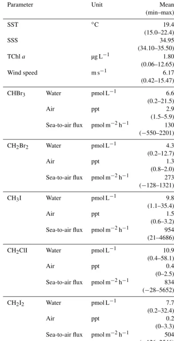
Table 1.Environmental parameters, as well as halocarbons in water, air and sea-to-air fluxes during the cruise. Means of sea surface temperature (SST), sea surface salinity (SSS) and wind speed are for 10 min averages. All data can be accessed at PANGAEA (Hep- ach et al., 2016).

Parameter Unit Mean

(min–max)

SST ^◦C 19.4

(15.0–22.4)

SSS 34.95

(34.10–35.50)

TChla µg L⁻¹ 1.80

(0.06–12.65)

Wind speed m s⁻¹ 6.17

(0.42–15.47)

CHBr₃ Water pmol L⁻¹ 6.6

(0.2–21.5)

Air ppt 2.9

(1.5–5.9) Sea-to-air flux pmol m⁻²h⁻¹ 130 (−550–2201)

CH₂Br₂ Water pmol L⁻¹ 4.3

(0.2–12.7)

Air ppt 1.3

(0.8–2.0) Sea-to-air flux pmol m⁻²h⁻¹ 273 (−128–1321)

CH₃I Water pmol L⁻¹ 9.8

(1.1–35.4)

Air ppt 1.5

(0.6–3.2) Sea-to-air flux pmol m⁻²h⁻¹ 954 (21–4686)

CH₂ClI Water pmol L⁻¹ 10.9

(0.4–58.1)

Air ppt 0.4

(0–2.5) Sea-to-air flux pmol m⁻²h⁻¹ 834 (−28–5652)

CH₂I₂ Water pmol L⁻¹ 7.7

(0.2–32.4)

Air ppt 0.2

(0–3.3) Sea-to-air flux pmol m⁻²h⁻¹ 504 (−126–2546)

fying different significant regions for halocarbon production.

Based on this criterion, four upwelling regions (I–IV) close to the coast were classified (Fig. 1). The most intense upwelling (lowest SSTs, high nutrient concentrations) appeared in the northernmost region of the cruise track, region I, while higher TChlaand lower nutrients indicate a fully developed bloom in the southern part of the cruise (upwelling regions III and IV). Upwelling region II was characterized by a lower

(6)

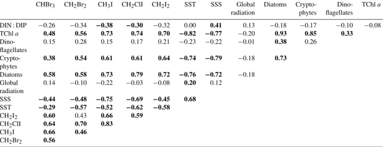
Table 2.Spearman’s rank correlation coefficients of correlations of all halocarbon surface data with several ambient parameters, as well as biological proxies. Bold numbers indicate correlations that are significant atp< 0.05 with a sample number of 107 for all environmental data and 46 for all phytoplankton and nutrient data considering all collocated surface data.

CHBr₃ CH₂Br₂ CH₃I CH₂ClI CH₂I₂ SST SSS Global Diatoms Crypto- Dino- TChla radiation phytes flagellates

DIN : DIP −0.26 −0.34 −0.38 −0.30 −0.32 0.00 0.41 0.13 −0.18 −0.17 −0.10 −0.08

TChla 0.48 0.56 0.73 0.74 0.70 −0.82 −0.77 −0.20 0.93 0.85 0.33

Dino- 0.15 0.28 0.15 0.17 0.21 −0.23 −0.22 −0.01 0.38 0.26

flagellates

Crypto- 0.38 0.54 0.61 0.61 0.64 −0.74 −0.79 −0.18 0.73

phytes

Diatoms 0.58 0.58 0.73 0.79 0.72 −0.76 −0.72 −0.18

Global 0.14 −0.10 −0.22 −0.03 −0.08 0.20 0.12

radiation

SSS −0.44 −0.48 −0.75 −0.69 −0.45 0.68 SST −0.29 −0.57 −0.52 −0.62 −0.58

CH₂I₂ 0.60 0.43 0.66 0.59

CH₂ClI 0.64 0.70 0.83

CH₃I 0.66 0.46

CH₂Br₂ 0.56

DIN : DIP ratio in contrast to region I. SSS with a mean of 34.95 (34.10 and 35.50) is lowest in upwelling region IV, which is likely influenced by local river input such as the rivers Pisco, Cañete and Matagente, and may explain the observed low salinities due to enhanced fresh water input in boreal winter (Bruland et al., 2005).

4 Halocarbons in the surface water and depth profiles during M91

4.1 Halocarbon distribution in surface water

Measurements of halocarbons in the tropical eastern Pa- cific are very sparse and no data were available for the Peruvian upwelling system before our campaign. Sea surface concentrations of CHBr₃ and CH₂Br₂ with means of 6.6 (0.2–21.5) and 4.3 (0.2–12.7) pmol L⁻¹, respectively, were measured during M91 (Table 1, Fig. 2). These values are low in comparison to 44.7 pmol L⁻¹CHBr₃in tropical upwelling systems in the Atlantic, while our measurements of CH2Br2 compare better to these upwelling systems, from which maximum concentrations of 9.4 pmol L⁻¹ were reported (Quack et al., 2007a; Carpenter et al., 2009;

Hepach et al., 2014, 2015). CHBr3(0.2–20.7 pmol L⁻¹) and CH₂Br₂ (0.7–6.5 pmol L⁻¹) concentrations in the tropical eastern Pacific open-ocean and Chilean coastal waters during a cruise from Punta Arenas, Chile, to Seattle, USA, in April 2010 (Liu et al., 2013) compare well with our data.

The most elevated concentrations measured at the Chilean coast agree with our elevated northern coastal data. Some measurements also exist for the tropical West Pacific with on average 0.5 to 3 times our CHBr₃and 0.2 to 1 times our CH₂Br₂, with the high average originating from a campaign

close to the coast with macroalgal and anthropogenic sources (Krüger and Quack, 2013; Fuhlbrügge et al., 2016b). CHBr3

and CH2Br2 have been suggested to have similar sources (Moore et al., 1996; Quack et al., 2007b). However, during our cruise, the correlation between the two compounds was comparatively weak (r_s=0.56), consistent with the findings of Liu et al. (2013), who ascribed the weaker correlation of these two compounds to formation in a common ecosystem rather than to the exact same biological sources. Maxima of CH₂Br₂were observed in both upwelling regions III and IV, while CHBr₃was highest in the most southerly upwelling IV (Fig. 2).

While we found the Peruvian upwelling and the adjacent waters to be only a moderate source region for bromocarbons, iodocarbons were observed in high concentrations of 10.9 (0.4–58.1), 9.8 (1.1–35.4) and 7.7 (0.2–32.4) pmol L⁻¹ for CH2ClI, CH3I and CH2I2, respectively (Table 1, Fig. 3a).

These concentrations identify the Peruvian upwelling as a significant source region of iodocarbons, especially considering the very short lifetimes of CH₂I₂(10 min) and CH₂ClI (9 h) in tropical surface water (Jones and Carpenter, 2005).

Hotspots were upwelling regions III and, even more so, the less fresh upwelling of region IV (Figs. 2 and 3).

The occurrence of CH₃I in the tropical oceans (up to 36.5 pmol L⁻¹) has previously been attributed to a predom- inantly photochemical source (Richter and Wallace, 2004;

Jones et al., 2010), explaining its global hotspots in the subtropical gyres and close to the tropical western boundaries of the continents (Ziska et al., 2013; Stemmler et al., 2014).

Previous campaigns in the eastern Pacific obtained concentrations of up to 21.7 and 8.8 pmol L⁻¹(Butler et al., 2007), and around 1.0 to 1.5 pmol L⁻¹(Mahajan et al., 2012), but not directly in the upwelling.

(7)

Figure 2.Halocarbon surface water measurements are shown in panels(a)and(b)for the bromocarbons (note the colour bar in the upper panel) with(a)CHBr₃and(b)CH₂Br₂. Iodocarbons can be found in panels(c–e)(note the colour bar in the lower panel) with(c)CH₃I, (d)CH₂ClI and(e)CH₂I₂.

15 17.5

20 22.5

25

0 15 30 45 60

09 11 13 15 17 19 21 23 25

0 1 2 3 4

0 300 600 900 1200

Days in December 2012

Iodocarbons in water [pmol L-1]Iodocarbons in air [ppt] SST [°C]Global radiation [W m-2]

III IV

CH₃I CH₂ClI

CH₂I₂ (a)

(b)

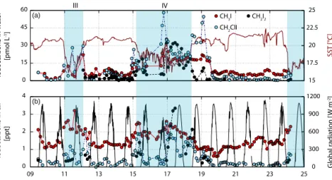
Figure 3.Surface water measurements of iodocarbons are presented in panel(a)with CH₃I in red, CH₂ClI in blue and CH₂I₂in black on the left side along with SST (dark red) on the right side. Additionally, atmospheric mixing ratios of CH₃I (red), CH₂ClI (blue) and CH₂I₂ (grey) on the left side together with global radiation (black, taken from pyranometer measurements referring to total shortwave radiation) on the right side are depicted in panel(b). Note that all times are in UTC.

No oceanic observations of CH2ClI and CH2I2have been published so far for the tropical eastern Pacific. Concentra- tions of CH2ClI of up to 24.5 pmol L⁻¹ were measured in the tropical and subtropical Atlantic Ocean (Abrahamsson et al., 2004; Chuck et al., 2005; Jones et al., 2010) and up to 17.1 pmol L⁻¹ for CH₂I₂(Jones et al., 2010; Hepach et al., 2015), which is lower but in the range of our measurements from the Peruvian upwelling.

Correlations between the compounds indicate similar sources for all measured halocarbons, except for CH2Br2, with upwelling region IV as a hotspot area (Fig. 2). The strongest correlation was found for CH3I with CH2ClI (rs= 0.83). CH2I2 and CH2ClI are often found to correlate very well with each other (Tokarczyk and Moore, 1994; Moore et al., 1996; Archer et al., 2007), which is usually attributed to the formation of CH₂ClI during photolysis of CH₂I₂. In com-

(8)

100 75 50 25

0 0 3 6 9 12

100 75 50 25

0 00 0.60.6 1.21.2 1.81.8 2.42.4 33

12 14 16 18 20 22

34.8 34.96 35.12

0 60 120 180 240 300 24 24.5 25 25.5 26 26.5

Temperature [°C]

Salinity Oxygen [µmol kg^-1] Potential density - 1000 [kg m^-3]

Fluorescence Total Chl a [µg L^-1] Phytoplankton [µg Chl a L^-1]

(d) ( f )

(e) (g)

84° W 78° W 72° W

20° S 10° S 0°

16 18 20 22 SST [°C]

(a)

Depth [m]

Cryptophytes x 100 Diatoms TChl a Fluorescence Oxygen Salinity Temperature CH₂ClI CH2I2

Density CH₃I

0 10 20 30 40

Halocarbons [pmol L^-1]

(b)

(c)

CH₂Br₂ CHBr₃

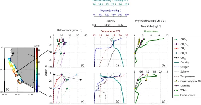
Figure 4.A cruise map including all CTD stations and SST is shown in panel(a), while selected depth profiles of iodocarbons and bromocarbons can be seen in panels(b–c), together with ambient parameters such as potential density (cyan), oxygen (dark blue), salinity (black) and temperature (dark red) in panels(d–e)and phytoplankton groups (cryptophytes and diatoms), total chlorophyllaand fluorescence in panels(f–g). CH₂I₂was undetectable at the first station (see also consistence with surface data). The data can be accessed at PANGAEA (Hepach et al., 2016).

parison, the weaker correlation between CH2ClI and CH2I2

(rs=0.59) during our cruise may be the result of additional sources for CH2ClI (see also Sect. 5).

4.2 Halocarbon distribution in depth profiles

Depth profiles of halocarbons reveal maxima at the surface and around the Chl a maximum, usually attributed to biological production of these compounds. CHBr₃and CH₂Br₂ profiles (Fig. 4a, b) showed distinct maxima in the deeper Chlamaximum during a large part of the cruise, while some profiles were characterized by elevated concentrations in the surface usually associated with upwelling water. Both kinds of profiles are consistent with previous studies finding maxima in the deeper water column in the open ocean and surface maxima in upwelling regions (Yamamoto et al., 2001;

Quack et al., 2004; Hepach et al., 2015). During the northern part of M91 (upwelling III), CH2Br2in the water column was more elevated than CHBr3(Fig. 4a), while CHBr3was usually higher during the remaining part of the cruise (Fig. 4b).

Though most of the stations were characterized by subsurface maxima of iodocarbons, which were mostly located between 10 and 50 m (see example in Fig. 4, upper panel), surface maxima were often observed in upwelling region IV (see example in Fig. 4, lower panel), the region with highest iodocarbon concentrations. Profiles with surface maxima were generally characterized by much higher concentrations of these compounds, although we cannot completely exclude

subsurface maxima at these locations owing to the sampling interval. CH2I2 was hardly detected in deeper water in the northern part of our measurements (Fig. 4, upper panel). Sur- face maxima in depth profiles of CH3I and CH2ClI were connected to surface maxima of several phytoplankton species, mainly diatoms (r_s=0.57 and 0.62). Direct and indirect biological and photochemical formation are considered possible sources for these maxima. CH₂I₂ was usually strongly depleted in the surface in contrast to the deeper layers due to its rapid photolysis, which may also have been a source for surface CH₂ClI. Subsurface maxima occurred both below and within the mixed layer (see the example in Fig. 4d indicated by the temperature, salinity and density profiles). Maxima in the mixed layer probably appear because of very fast production (Hepach et al., 2015), while maxima below the mixed layer are supported by accumulation due to reduced mixing.

All five halocarbons were strongly depleted in waters below 50 m. These deeper layers were also characterized by very low oxygen values, known as strong OMZ below the biologically active layers (Karstensen et al., 2008). A possible reason for the strong depletion of the halocarbons is their bacterially mediated reductive dehalogenation occurring under anaerobic conditions (Bouwer et al., 1981; Tanhua et al., 1996).

(9)

5 Relationship of surface halocarbons to environmental parameters

Physical and chemical parameters as well as biological proxies such as TChl a and phytoplankton group composition were investigated using correlation analysis in order to ex- amine marine sources of halocarbons.

5.1 Potential bromocarbon sources

Bromocarbons were weakly but significantly anticorrelated with SSS and SST (r_s between−0.29 and−0.57), indicating sources in the upwelled water (Table 2). They showed a positive correlation with diatoms (r_s=0.58 for both compounds), the dominant phytoplankton group in the region.

Diatoms have already been found to be involved in bromocarbon production in several laboratory and field studies (Tokarczyk and Moore, 1994; Moore et al., 1996; Quack et al., 2007b; Hughes et al., 2013). Thus, these findings are in agreement with current assumptions that this group may contribute directly or indirectly to bromocarbon production.

During M91, CH₂Br₂was more abundant in cooler, nutrient- rich water than CHBr₃, leading to a stronger correlation with TChla and SST, indicating an additional source associated with fresh upwelling. No significant correlations were found for bromocarbons with polysaccharidic DOM (Table 3), im- plying that DOM components analysed during the cruise were not involved in bromocarbon production, at least not in the upper water column. Bromocarbon production from DOM has also been suggested to be slow (Liu et al., 2015), which could shift larger bromocarbon concentrations to later times after our cruise.

5.2 Iodinated compounds and phytoplankton

In general, the iodocarbons correlated more strongly with biological parameters than the bromocarbons. Diatoms were found to correlate very strongly with all three iodocarbons (r_s=0.73 with CH₃I,r_s=0.79 with CH₂ClI andr_s=0.72).

Weak but significant anticorrelations with DIN : DIP and SST suggest that iodocarbons were associated with cool and slightly DIN depleted water. The occurrence of large amounts of iodocarbons seemed to be associated with an es- tablished diatom bloom. The production of CH₃I, CH₂ClI and CH2I2by a number of diatom species has been observed in several studies before (Moore et al., 1996; Manley and de la Cuesta, 1997), consistent with our findings. The very high correlation of cryptophytes with iodocarbons was likely based on the co-occurrence of these species with diatoms (Table 2 and description in Sect. 3).

5.3 Iodinated compounds and DOM

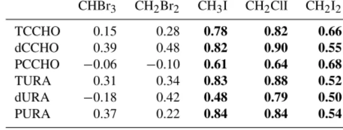
Correlations of the three iodinated compounds with polysaccharidic DOM components in subsurface water revealed a strong relationship of the iodocarbon abundance with

Table 3. Correlations of halocarbons with combined high- molecular-weight (HMW) carbohydrates (CCHO) and uronic acids (URA) from subsurface samples (T – total; d – dissolved; P – particulate) with a sample number of 29 for each variable. Bold numbers indicate significant correlations.

CHBr₃ CH₂Br₂ CH₃I CH₂ClI CH₂I₂

TCCHO 0.15 0.28 0.78 0.82 0.66

dCCHO 0.39 0.48 0.82 0.90 0.55

PCCHO −0.06 −0.10 0.61 0.64 0.68

TURA 0.31 0.34 0.83 0.88 0.52

dURA −0.18 0.42 0.48 0.79 0.50

PURA 0.37 0.22 0.84 0.84 0.54

polysaccharides and in particular uronic acids (Table 3).

CH₃I and CH₂ClI showed strong correlations with particulate uronic acids (bothrs=0.84), total uronic acids (r_s= 0.83 and 0.88) and dissolved polysaccharides (r_s=0.82 and 0.90). The correlations of CH₂I₂with polysaccharides were less strong but significant (r_s=0.68 with particulate, r_s= 0.66 with total and r_s=0.55 with dissolved). The above- listed DOM components were also significantly correlated to diatoms (r_s=0.68 with polysaccharides andr_s=0.75 with uronic acids), which were a potential source for the accumu- lated organic matter in the subsurface. The exact composition of surface water DOM is determined by ecosystem composi- tions. Polysaccharides with uronic acids as an important con- stituent have for example been shown to contribute largely to the DOM pool in a diatom-rich region (Engel et al., 2012).

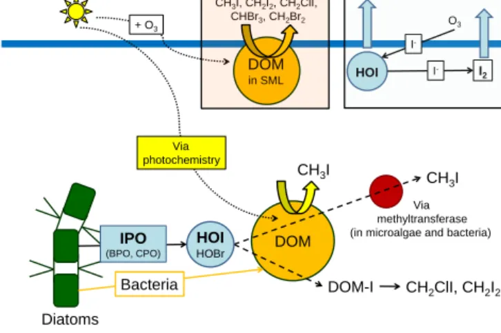
Hill and Manley (2009) tested several diatom species for their production of halocarbons in a laboratory study, and suggested that a major formation pathway for polyhalo- genated compounds may actually not be from direct algal production but rather indirectly through their release of hypoiodous (HOI) and hypobromous acid (HOBr), which then react with the present DOM (Lin and Manley, 2012; Liu et al., 2015). The formation of HOI and HOBr within the algae is enzymatic, with possible chloroperoxidase (CPO), BPO and iodoperoxidase (IPO) involvement. While CPO and BPO may produce both HOBr and HOI, IPO only leads to HOI.

Moore et al. (1996) suggested that the occurrence of BPO and IPO in the phytoplankton cells may be highly species- dependent. This leads to the assumption that diatoms abundant in the Peruvian upwelling contained more IPO than BPO, which could explain the higher abundance of iodocarbons relative to bromocarbons during M91.

The formation of CH₃I through DOM may be different than the production of CH₂ClI and CH₂I₂. While CH₂I₂is suggested to be formed via haloform-type reactions (Car- penter et al., 2005), CH₃I is produced using a methyl-radical source (White, 1982). The relationship of CH₃I with DOM can be the result of both photochemical and biological production pathways: DOM, which was observed in high concentrations in the biologically productive waters, can act as

(10)

the methyl-radical source during photochemical production of CH₃I (Bell et al., 2002). A second possible biological pathway of methyl iodide production takes place via bacteria and microalgae, which can utilize methyl transferases in their cells. HOI plays a significant role in this production pathway by providing the iodine to the methyl group (Yokouchi et al., 2014).

The Peruvian upwelling was a strong source for the iodocarbons CH₃I, CH₂ClI and CH₂I₂and a weaker source for the bromocarbons CHBr₃ and CH₂Br₂. We propose a formation mechanism for this region as described in Fig. 5 based on measurements of short-lived halocarbons and biological parameters during M91. Diatoms, which can contain the necessary enzymes for halocarbon formation, were identified as an important source based on their strong correlations with the bromo- and iodocarbons and with polysaccharidic DOM. The very good correlations of iodocarbons with polysaccharides and uronic acids are an indicator that these DOM components may have been important substrates for iodocarbon production potentially produced from the present diatoms. The higher iodocarbon concentrations can likely be explained by phytoplankton species containing more IPO than BPO, leading to a stronger production of iodocarbons.

Additionally, the particular type of DOM may also have regu- lated the production of specific halocarbons (Liu et al., 2015), in this case CH₃I, CH₂ClI and CH₂I₂.

One interesting feature of our analysis is the fact that CH2I2, when compared to the other two iodocarbons, showed weaker correlations with the polysaccharides possibly due to its shorter surface water lifetime. Moreover, CH2I2 and CH2ClI showed weaker correlations in the Peruvian upwelling than during other cruises in the tropical Atlantic, namely MSM18/3 (Hepach et al., 2015) and DRIVE (Hep- ach et al., 2014). When combining the two arguments of a short CH₂I₂ lifetime and only a weak correlation between CH₂I₂and CH₂ClI, this may indicate an additional source for CH₂ClI similar to CH₃I, explaining why CH₃I and CH₂ClI correlate much better with each other than with CH₂I₂.

6 From the ocean to the atmosphere 6.1 Sea-to-air fluxes of iodocarbons

Due to high oceanic iodocarbon concentrations measured in sea surface water of the Peruvian upwelling and despite the moderate prevailing wind speeds of 6.17 (0.42–

15.47) m s⁻¹, high iodocarbon sea-to-air fluxes were calculated in contrast to the rather low bromocarbon emissions during our cruise (Fuhlbrügge et al., 2016a). The highest average fluxes of the three iodocarbons of 954 (21–

4686) pmol m⁻²h⁻¹ were calculated for CH₃I, followed by 834 (−24–5652) pmol m⁻²h⁻¹ for CH₂ClI and finally 504 (−126–2546) pmol m⁻²h⁻¹for CH₂I₂(Table 1). These were on average 4 to 7 times higher than CHBr₃ and 2 to

DOM

DOM-I CH₂ClI, CH₂I₂ Diatoms

CH₃I

V ia methyltransferase (in microalgae and bacteria)

CH₃I

CH₃I, CH₂I₂, CH₂ClI, CHBr₃, CH₂Br₂

HOI

HOBr

DOM HOI in SML

Via photochemistry

Bacteria IPO

(BPO, CPO)

O₃ + O3

I^- I^- I₂

Figure 5.Proposed mechanisms for formation of iodocarbons – release of HOI with the help of iodoperoxiases (IPO), followed by re- action with DOM (dissolved organic matter (DOM) via iodine bind- ing to DOM (DOM-I) to form CH₂ClI and CH₂I₂. CH₃I forms via photochemistry and/or biological formation via methyltransferases.

The box indicates potential formation of halocarbons from DOM in the sea surface microlayer (SML) in addition to inorganic iodine sources there, shown by the light-blue box. For more information on the inorganic iodine chemistry in the SML, please refer to Carpenter et al. (2013).

4 times higher than the CH2Br2sea-to-air fluxes during the cruise.

Our estimated fluxes of CH3I are in the range of emissions calculated for the tropical and subtropical Atlantic of 625 to 2154 pmol m⁻²h⁻¹(Chuck et al., 2005; Jones et al., 2010). Moore and Groszko (1999), who performed a study between 40^◦N and 40^◦S close to our investigation region but not covering the Peruvian upwelling, calculated on average 666 pmol m⁻²h⁻¹, which is 0.7 times our flux. Sea- to-air fluxes of CH₂ClI from the same studies were reported to range on average between 250 and 1138 pmol m⁻²h⁻¹, with the largest fluxes originating from the Mauritanian upwelling region. These are 0.3 to 1.4 times the fluxes we calculated, showing that the Peruvian upwelling region is at the top end of oceanic CH₂ClI emissions. We are only aware of two studies focusing on emissions of CH2I2from the tropical Atlantic Ocean (Jones et al., 2010; Hepach et al., 2015); these studies show on average 0.2 and 1.4 times, respectively, the fluxes from the tropical eastern Pacific. The larger sea-to-air fluxes reported in Hepach et al. (2015) from the equatorial Atlantic cold tongue are mainly a result of much lower atmospheric mixing ratios there, increasing the concentration gradient, and additionally higher wind speeds, increasing the exchange coefficientk_w.

In summary for this section, the large production of iodocarbons in the Peruvian upwelling led to enhanced emissions of these compounds to the troposphere despite very low wind speeds. An additional factor influencing halocarbon emissions is the low height and insolation of the MABL,

(11)

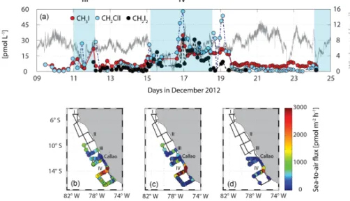
Figure 6.The concentration gradient of CH₃I, CH₂ClI and CH₂I₂along with wind speed (grey) is shown in panel(a), while the sea-to-air flux is depicted in panel(b)for CH₃I,(c)for CH₂ClI and(d)for CH₂I₂. Note the colour bar on the right.

0 10 20 30 40 50 60 0

1 2 3 4

CH₃I in water [pmol L^-1] (a)

Atmospheric iodocarbons [ppt]

0 10 20 30 40 50 60 CH₂ClI in water [pmol L^-1]

(b)

r = 0.68 r = 0.50 r = 0.24

r = 0.27

0 10 20 30 40 50 60 CH₂I₂ in water [pmol L^-1]

(c)

r = 0.40 r = 0.92

CH₃I, day CH₃I, night

CH2ClI, day CH₂ClI, night

CH₂I₂, day CH₂I₂, night

Figure 7. Atmospheric iodocarbons vs. oceanic iodocarbons for CH₃I (a), CH₂ClI(b) and CH₂I₂ (c), with the filled and open circles representing data obtained during the daytime and night-time, respectively, including least-squares lines (solid for day, dashed for night).

where halocarbons accumulate above the air–sea interface.

The large sea-to-air fluxes and low wind speeds should result in high tropospheric iodocarbons, which was indeed observed and is discussed in the following section.

6.2 Atmospheric iodocarbons

Atmospheric mixing ratios of the three iodocarbons were elevated during M91, with up to 3.2 ppt for CH3I, up to 2.5 ppt for CH2ClI and up to 3.3 ppt for CH2I2 (Table 1, Fig. 6), likely a result of the strong production and emissions of these compounds.

CH₃I data were generally elevated in comparison to other eastern Pacific measurements of up to 1.1 to 2.1 ppt CH₃I (Butler et al., 2007; Mahajan, et al., 2012), but lower than in the tropical central and eastern Atlantic around the equa- tor, characterized by higher atmospheric CH₃I of over 5 ppt (Ziska et al., 2013). Gómez Martin et al. (2013) report 1.7 times higher maximum mixing ratios of CH₃I of 5.4 ppt from the Galápagos Islands, possibly rather influenced by very local sources around the measuring site, e.g. from sea-

weed or macroalgae. Both CH₂ClI and CH₂I₂ were also elevated in comparison to previous oceanic measurements, where, for example, 0.01 to 0.99 ppt CH₂ClI was measured for remote locations in the Atlantic and Pacific (Chuck et al., 2005; Varner et al., 2008) and only up to 0.07 ppt was reported for CH2I2 at a remote site in the Pacific (Yokouchi et al., 2011). Coastal areas with high macroalgal abundance were characterized by high CH2ClI of up to 3.4 ppt (Varner et al., 2008) and up to 3.1 ppt CH2I2(Carpenter et al., 1999;

Peters et al., 2005), while 19.8 ppt (Peters et al., 2005) was measured at Mace Head, Ireland, and Lilia, France, in the North Atlantic.

The different atmospheric lifetimes of the three iodocarbons, ranging between 4 days (CH₃I), 9 h (CH₂ClI) and 10 min (CH₂I₂) (Carpenter and Reimann, 2014), partly explain the observed differences in their distributions. Although atmospheric CH₃I was generally elevated in regions of high oceanic CH₃I (Fig. 3) in upwelling regions III and IV, the atmospheric and oceanic data did not show a significant correlation. The CH3I lifetime of several days allows atmospheric

(12)

CH3I to mix within the MABL, possibly masking a correlation between local source regions and elevated mixing ratios.

The two shorter-lived iodinated compounds CH₂ClI and CH₂I₂ generally showed a stronger influence of local marine sources. Both species correlate significantly with their oceanic concentrations with r_s=0.60 (CH₂ClI) and r_s= 0.64 (CH₂I₂). Oceanic CH₂ClI and CH₂I₂were emitted into the boundary layer, where they could accumulate during the night (see comparison with global radiation in Fig. 3b) and were rapidly degraded during the daytime via photolysis, which is their main sink in the troposphere (Carpenter and Reimann, 2014). This accumulation is especially apparent when the data are separated into “day” and “night” according to global radiation measurements, assuming that no radiation implies complete darkness. During the day, oceanic CH2ClI and CH2I2correlate weakly withr=0.5 for CH2ClI and no significant correlation was found for CH₂I₂ (r=0.4), also owing to the fact that hardly any CH₂I₂was measured during daylight. However, oceanic CH₂ClI and CH₂I₂correlate significantly with their atmospheric counterparts withr=0.68 and 0.92 in the night hours (Fig. 7). Moderate average wind speeds in the upwelling regions (Fig. 6) and stable atmospheric boundary layer conditions (Fuhlbrügge et al., 2016a) supported the accumulation of these compounds.

The Peruvian upwelling was in general characterized by elevated atmospheric iodocarbons as a result of their large sea-to-air fluxes caused by strong biological production. The upwelling could sustain elevated atmospheric levels of, for example, CH3I, trapped iodocarbons and their degradation products in a stable MABL, and may have therefore contributed significantly to the tropospheric inorganic iodine budget, which is discussed in the following.

6.3 Contributions to tropospheric iodine

After their emission from the ocean and their chemical degradation in the marine boundary layer, iodocarbons contribute to the atmospheric inorganic iodine budget, I_y. The impor- tance of this contribution compared to abiotic sources is cur- rently under debate and analysed for various oceanic environments (Mahajan et al., 2010; Großmann et al., 2013;

Prados-Roman et al., 2015). So far, no correlations of IO with organic iodine precursor species have been observed (Großmann et al., 2013) and correlations between IO and Chlawere often found to be negative (Mahajan et al., 2012;

Gómez Martín et al., 2013). Chemical modelling studies, un- dertaken to explain the contributions of organic and inorganic oceanic iodine sources, showed in simulations that only a small fraction of the atmospheric IO stems from the organic precursors, with estimates of about 25 % on a global average (Prados-Roman et al., 2015). Both arguments, the miss- ing correlations and the small contributions, indicate that the organic source gas emissions play a minor role for the atmospheric iodine budget. Given the special conditions of the Pe- ruvian upwelling with cold, nutrient-rich waters, the strong

iodocarbon sources, and a stable MABL and trade inversion, it is of interest to analyse the local contributions to the atmosphere in this region and to compare with estimates from other oceanic environments.

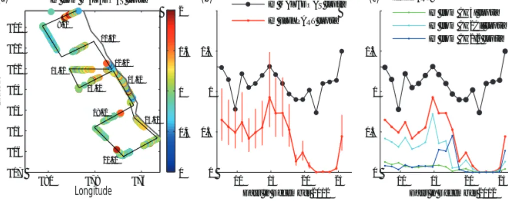
We focus our analysis on the section of the cruise where MAX-DOAS measurements of IO and simultaneous iodocarbon measurements in the surface water and atmosphere were made (roughly south of 10^◦S). Tropospheric vertical column densities (VCDs) of IO in the range of 2.5–

6.0×10¹²molec. cm⁻²were inferred from the MAX-DOAS measurements. Similar VCDs of IO were reported by Schön- hardt et al. (2008) based on remote satellite measurements from SCIAMACHY, but VCDs around 1 order of magnitude higher were measured by Mahajan et al. (2012), which was, however, considerably further from the coast located than our measurements. Volume mixing ratios of IO along the cruise track (Fig. 8a) derived from the MAX-DOAS measurements show a pronounced variability and maxima close to upwelling regions II and IV. Daytime averaged IO volume mixing ratios are displayed in Fig. 8b and range between 0.8 (on 12 and 22 December) and 1.5 ppt (on 26 December).

Overall, the daytime IO abundance in the MABL above the Peruvian upwelling was relatively high compared to measurements from the nearby Galápagos Islands (∼0.4 ppt) (Gómez Martín et al., 2013), and measurements closer to our investigation region with around between 0.2 and 0.6 ppt in the MABL (Dix et al., 2013; Wang et al., 2015), as well as from other tropical oceans such as the Malaspina 2010 circumnavigation (0.4–1 ppt) (Prados-Roman et al., 2015).

Other measurement campaigns such as the Cape Verde measurements (Read et al., 2008) and the TransBromSonnein the western Pacific (Großmann et al., 2013) found similar IO mixing ratios with values above 1 ppt, but significantly lower IO VCDs in the latter case. One of the first measurements of IO above the Peruvian upwelling was conducted by Volkamer et al. (2010), who report up to 3.5 ppt in the region.

These larger mixing ratios in comparison to our study are possibly due to even more enhanced biological production as the upwelling is more much more pronounced in October than in late December.

The M91 cruise track crisscrossed the waters between the coast and 200 km offshore multiple times, providing a com- prehensive set of measurements over a confined area (see Fig. 8a) and allowing us to analyse the relation between IO and organic precursors. Assuming constant emissions over the cruise period we can link the oceanic sources with atmospheric IO observations at locations reached after hours to days of atmospheric transport. Therefore, we released FLEX- PART trajectories from all sea surface measurement locations continuously over the whole measurement time period from 8 to 26 December loaded with the oceanic iodine as prescribed by the observed iodocarbon emissions. Based on the simulations of transport and chemical decay described in Sect. 2.5, we derived organic and inorganic iodine mixing ratios individually for each air parcel. Mixing with air