HOAPS and ERA-Interim precipitation over the sea: validation against shipboard in situ measurements

(1)

www.atmos-meas-tech.net/9/2409/2016/

doi:10.5194/amt-9-2409-2016

HOAPS and ERA-Interim precipitation over the sea: validation against shipboard in situ measurements

Karl Bumke¹, Gert König-Langlo², Julian Kinzel^1,3, and Marc Schröder³

1GEOMAR Helmholtz Centre for Ocean Research Kiel, 24105 Kiel, Germany

2Alfred Wegener Institute Helmholtz Centre for Polar and Marine Research, 27570 Bremerhaven, Germany

3Deutscher Wetterdienst, Satellite Based Climate Monitoring, 63067 Offenbach, Germany Correspondence to:Karl Bumke (kbumke@geomar.de)

Received: 21 January 2016 – Published in Atmos. Meas. Tech. Discuss.: 5 February 2016 Revised: 13 May 2016 – Accepted: 17 May 2016 – Published: 1 June 2016

Abstract. The satellite-derived HOAPS (Hamburg Ocean Atmosphere Parameters and Fluxes from Satellite Data) and ECMWF (European Centre for Medium-Range Weather Forecasts) ERA-Interim reanalysis data sets have been validated against in situ precipitation measurements from ship rain gauges and optical disdrometers over the open ocean by applying a statistical analysis for binary estimates. For this purpose collocated pairs of data were merged within a certain temporal and spatial threshold into single events, according to the satellites’ overpass, the observation and the ERA- Interim times. HOAPS detects the frequency of precipitation well, while ERA-Interim strongly overestimates it, especially in the tropics and subtropics. Although precipitation rates are difficult to compare because along-track point measurements are collocated with areal estimates and the number of available data are limited, we find that HOAPS underestimates precipitation rates, while ERA-Interim’s Atlantic-wide average precipitation rate is close to measurements. However, when regionally averaged over latitudinal belts, deviations between the observed mean precipitation rates and ERA- Interim exist. The most obvious ERA-Interim feature is an overestimation of precipitation in the area of the intertropical convergence zone and the southern subtropics over the At- lantic Ocean. For a limited number of snow measurements by optical disdrometers, it can be concluded that both HOAPS and ERA-Interim are suitable for detecting the occurrence of solid precipitation.

1 Introduction

Precipitation is one of the key parameters of the global water cycle. Therein the precipitation over the ocean is especially important since it contributes more than 75 % of the global annual total precipitation (Schmitt, 2008). Due to climate change it is reasonable to expect changes in both the pattern and amount of precipitation (Liu and Allan, 2013;

O’Gorman et al., 2012; Trenberth, 2011), as indicated by changes in the horizontal surface salinity distribution over the ocean (Durack et al., 2012). However, Valdivieso and Haines (2011) calculated that near the surface, much of the Atlantic is generally saltier compared to the climatology, although not uniformly so. They suspect that precipitation from the ERA-Interim (Dee et al., 2011) product might have errors.

On the other hand, Grist et al. (2014) found that a large part of the spread in the estimates of the mean surface-forced circulation of the subtropics is associated with biases in the global ocean heat budgets implied by the atmospheric reanalyses. Indeed, for saltiness an unbiased estimate of freshwater fluxes is needed; good knowledge about evaporation is also essential. Regarding precipitation, robust trends in re- gional precipitation over the ocean have not been detected to date because in situ precipitation measurements are sparse and uncertain (Rhein et al., 2013). However, the progress in satellite technology has provided the possibility of retriev- ing global data sets from space, including precipitation. In addition to the Hamburg Ocean Atmosphere Parameters and Fluxes from Satellite data (HOAPS, Andersson et al., 2010, 2011), remote-sensing-based precipitation data sets are al- ternatively available, e.g. from the GPCP (Global Precipi-

(2)

tation Climatology Project, see e.g. Huffman et al., 1997), CMorph (Climate Prediction Center MORPHing technique, Joyce et al., 2004), TMPA (TRMM Multisatellite Precipita- tion Analysis, Huffman et al., 2007), Persiann (Precipitation Estimation from Remotely Sensed Information using Neu- ral Networks, Behrangi et al., 2009), the HSAF (Hydrology Satellite Application Facility precipitation products, Mugnai et al., 2013) or IMERG (Integrated Multi-satellitE Retrievals for Global precipitation measurement, Huffman et al., 2015).

However, concerns have been expressed over the need for further work to evaluate these data sets (Rhein et al., 2013).

Recent progress in reanalyses shows improved accuracy in precipitation (Dee et al., 2011), although tests for internal consistency among different components of the hydrological cycle in reanalysis data still reveal some issues (Tren- berth, 2011). This is supported by a study of Andersson et al. (2011), who pointed out that state-of-the-art satellite retrievals and reanalysis data sets still disagree on global precipitation amounts, patterns, variability and temporal behaviour, with the relative differences increasing in the pole- ward direction. Pfeifroth et al. (2013) showed that HOAPS tends to underestimate precipitation by 6 to 9 % in the tropical Pacific, where ERA-Interim (Dee et al., 2011) gives an overestimation of 8 to 10 %. Note that these comparisons were done against measurements on atolls, although the rep- resentativeness of the atoll gauges of open-ocean rainfall is still an unanswered question (Wang et al., 2014). Andersson et al. (2011) have shown that HOAPS gives lower precipitation rates than ERA-Interim, except for small areas in the northern subtropics, the north-western and south-western At- lantic Ocean. They also figured out that over the mid–high latitudes between 40 and 70^◦, the precipitation (only liquid precipitation) in GPCP (Adler et al., 2003) is also systemati- cally 10–30 % higher relative to HOAPS. Locally the values exceed 50 %. North of 60^◦N, Lindsay et al. (2014) detected an overestimation in monthly precipitation in ERA-Interim, ranging from 10 to 25 %. Kidd et al. (2013) found that precipitation in the tropical Atlantic is skewed to the east towards the African coast by ERA-Interim. On the other hand, several studies have shown that in the area of the Iberian Peninsula (Belo-Pereira et al., 2011) or in the area of four African river basins (Thiemig et al., 2012), ERA-Interim overestimates the frequency of rain events as well.

Furthermore, with respect to solid precipitation, Klepp et al. (2010) demonstrated the ability of HOAPS to detect even light amounts of cold season snowfall, with a high accuracy (96 %) between point-to-area collocations of ship-based optical disdrometer data (ODM 470) and HOAPS data.

In the present study we use in situ ship rain gauge (Hasse et al., 1998) and optical disdrometer (ODM 470) data (Großk- laus et al., 1998), gained on board research vessels, to vali- date two data sets, the HOAPS and the ECMWF (European Centre for Medium-Range Weather Forecasts) ERA-Interim reanalysis data set. For the present study HOAPS has been chosen as an example of a satellite-derived precipitation esti-

mate, because it is only derived from SSM/I (Special Sensor Microwave Imager) radiometers in their native sensor resolution without any further interpolation. Section 2 gives an overview of the data and instruments used. The collocation of the data is described in Sect. 3, followed by an overview of validation methods used in Sect. 4. In Sect. 5 we present our results, followed by a discussion of the results and the summary and outlook in Sects. 6 and 7.

2 Data

For this study data from two measurement periods, 1995 to 1997 and 2005 to 2008, are available.

The 1995 to 1997 data were collected on the German ship R/V Meteor using a ship rain gauge (SRG, Hasse et al., 1998), on board the German R/V Polarstern, the US R/V Knorrand the US R/VRon Brownusing optical disdrometers (ODM 470, Großklaus et al., 1998). During this period the ODM 470s were coupled with opto-electronic infrared rain sensors, switching the sensors on with the onset of precipitation and switching them off about 30 min after the last precipitation occurrence. Due to reported sporadic malfunc- tions of the rain sensor we use only periods, when ODM data are available and did not assume that there was generally no precipitation along the track when ODMs were switched off.

Measurements are available at 8 min intervals. Data were collected over the Atlantic Ocean and the tropical Pacific Ocean.

For 2005 to 2008, SRG data are available, collected on board the German R/VPolarsternand R/VMaria S. Merian (Bundesamt für Seeschifffahrt und Hydrographie, 2015). A description of the meteorological observatory ofPolarstern can be found in König-Langlo et al. (2006). In contrast to the earlier period, the instruments were run continuously. Mea- surement intervals are 10 min. Data are collected mostly over the Atlantic Ocean.

2.1 Ship rain gauge measurements

The SRG is commercially available from Eigenbrodt Envi- ronmental Measurement Systems near Hamburg, Germany.

An outstanding feature of the SRG is an additional lateral collector, which is especially effective under high wind speed conditions (Hasse et al., 1998). Collected water, estimated separately from the top and lateral collector, in combination with measured wind speeds relative to the instrument, allows the derivation of true rainfall rates (Clemens, 2002). Compar- isons to other instruments show that the SRG performs well and gives nearly unbiased estimates of rainfall (Clemens and Bumke, 2002).

Position and time at the end of each measurement interval were taken from the ship’s measurement system. Mea- surement intervals were set to 8 min for R/VMeteor(1995–

1997), while R/VPolarsterndata (2005–2008) are available for 10 min intervals. R/VMaria S. Meriandata (2007–2008)

(3)

Figure 1.Comparison of simultaneous measurements of precipitation (rain only) on board R/VAlkorin the Baltic Sea (data from 1999 to 2005, May to October) using an ODM 470 and a SRG. The interval of measurements is 1 min.

have been integrated over 10 min, based on 1 min measurement intervals. Since SRGs are not suitable for measuring snow, only data collected at air temperatures above 4^◦C have been used. Long-term measurements on the main building of the GEOMAR Helmholtz Centre for Ocean Research Kiel, Germany, have shown that nearly all discrepancies between ODM 470 measurements, which give extreme high precipitation rates using the rain algorithm in case of solid precipitation, and SRG measurements, occur at temperatures below 4^◦C, which is in agreement with a study of Froidurot et al.

(2014).

2.2 Shipboard ODM 470 optical disdrometer measurements

The ODM 470 (Großklaus et al., 1998) is also commercially available from Eigenbrodt Environmental Measurement Sys- tems. It was successfully validated to measure precipitation, even under strong wind conditions (Großklaus, 1996; Bumke et al., 2004). Lempio et al. (2007) further developed the snowfall algorithm and applied it to ODM 470 measurements during an intercomparison field campaign in Uppsala, Swe- den, during winter 1999/2000. Comparison with gauge data and daily manual measurements showed reliable instrument performance. The correlation coefficient for 56 days of manual measurements wasr=0.794.

The measurement principle of the ODM 470 is light ex- tinction caused by hydrometeors passing through a cylindri- cal sensitive volume, which is kept perpendicular to the local wind direction with the aid of a wind vane. The local wind speed is measured using a cup anemometer. The disdrometer measures the size of the cross-sectional area and the resi- dence time of hydrometeors in the sensitive volume, within a size range with a diameter of 0.4–22 mm (snow version) and 0.5–6.4 mm (rain version). Measurements are partitioned

into 128 size bins, with the highest resolution at small particles and a logarithmic increase in size (snow version) or constant resolution and a linear increase in size (rain version).

Coincidence effects of multiple hydrometeors, within the sensitive volume at the same time and edge effects of partly scanned hydrometeors, are considered in the same way for liquid- and solid-phase precipitation. The precipitation rate in mm h⁻¹is calculated using the size bins, terminal velocity, mass of the hydrometeors and local wind speed (Clemens, 2002). The determination of the rainfall rate through the liquid water content (mass) and the fall velocity is easily pa- rameterized, as rain drops have a nearly spherical shape and constant density. In contrast to rainfall, solid precipitation is characterized by a variety of complex shapes with different fall velocities and different equivalent liquid water contents.

The measured cross-sectional area depends on the size, shape and orientation of the solid particles hindering the develop- ment of a unique solid precipitation retrieval scheme. The re- lationship between mass or equivalent liquid water content and the terminal fall velocity for snow crystals was anal- ysed by Hogan (1994) as a function of their maximum dimension. However, the disdrometer measures the size of the cross-sectional area instead of the maximum dimension of non-spherical particles. Assuming that the ice crystals fall randomly oriented through the sensitive volume (Brandes et al., 2007), Lempio et al. (2007) found from theoretical ex- periments using a ray tracing model (Macke et al., 1998) that the products of the terminal velocity and the equivalent liquid water content, as a function of the cross-sectional area, for different types of snow crystals are of the same order of mag- nitude. That allows one common parameterization to be used for all kinds of crystals; for practical reasons, lump graupel was chosen. As it is nearly spherical in shape, it needs no transformation function from cross-sectional area to maximum dimension. The parameterization for lump graupel, which was the most frequently observed precipitation type over the Nordic Seas during the LOFZY campaign (Klepp et al., 2010), is applicable for particles with a size range of 0.4–

9 mm. The snow version of the ODM 470 was mounted on R/VKnorrand R/VPolarstern, the rain version on R/VRon Brown. While all measurements on R/VKnorr(only 1997) were snow measurements, synoptic observations of the on- board weather station operated by the German Meteorologi- cal Service have been used for R/VPolarsternmeasurements (period 1995–1997), to decide whether precipitation was of liquid or solid phase (König-Langlo et al., 2006). Measure- ments on R/VRon Brown(only 1997) are rain measurements only. Precipitation rates are estimated from disdrometer data as 8 min time series. A comparison of simultaneous rainfall- only measurements on board R/VAlkor, using a disdrometer and a SRG based on 1 min time series, is given in Fig. 1. The correlation coefficient is 0.9 and the agreement in terms of accumulated rain is excellent, with a deviation of less than 5 %.

(4)

2.3 HOAPS

The satellite-derived HOAPS climatology is a compilation of precipitation and evaporation data with the goal of es- timating the net freshwater flux from one consistently derived global satellite data set over the global ice-free oceans.

To achieve this goal, HOAPS utilizes multi-satellite averages, inter-sensor calibration and an efficient sea-ice detection procedure. In the utilized version all HOAPS variables are derived using radiances from the Special Sensor Microwave/Imager (SSM/I) radiometers, except for the sea surface temperature, which is obtained from the Advanced Very High Resolution Radiometer (AVHRR) measurements (Andersson et al., 2010). Three data subsets of HOAPS- 3.0 are available over the period 1987 to 2008, compris- ing scan-based pixel-level data (HOAPS-S) and two types of gridded data products (HOAPS-G and HOAPS-C), which make HOAPS useful for a wide range of applications. The HOAPS-S data set, used in the present study, contains all retrieved physical parameters at the native SSM/I pixel-level resolution of approximately 50 km. The HOAPS-3.0 precipitation retrieval is based on a neural network, also described in Andersson et al. (2010).

The detection of very light rain below 0.3 mm h⁻¹is ham- pered by the sensitivity of the microwave imager. In the HOAPS precipitation algorithm a precipitation signal below the threshold value is set to zero. From experience with the preceding HOAPS precipitation algorithm, a value of 0.3 mm h⁻¹turned out to be an appropriate limit for distin- guishing between a real precipitation signal and background noise (Andersson et al., 2010). The algorithm does not dis- criminate between rain and snowfall. Due to the strong influ- ence of increasing emissivity near land and sea-ice-covered areas, HOAPS is devoid of data within 50 km off any coast- line or sea ice. Therefore ship data within the coastal zones are neglected, too. All individual descending and ascending overpasses of the SSM/I radiometers are used for the ground validation. The position of the HOAPS data represents the centre of an instantaneous field of view, which is about 50 km in diameter.

2.4 ECMWF ERA-Interim

ECMWF ERA-Interim reanalysis (Dee et al., 2011) was initiated in 2006 and represents the latest global atmospheric reanalysis created by the ECMWF. It covers the time period from 1979 onwards and is continuously updated on a monthly basis in near-real time. The ERA-Interim reanalysis is produced by means of a 4-D variational data assimilation scheme, which advances forward in time using 12- hourly analysis cycles (Dee et al., 2011). An implemented forecast model estimates the evolving state of the global atmosphere and surface, and is then constrained by observations of various types and multiple sources as well as a background estimate of the model. Near-surface parameters are

then derived subsequently to upper-air atmospheric fields, both of which serve as a basis for initializing a short-range model forecast that produces a prior state estimate for the successive time step. The short-range forecast, constituting the final part of the ECMWF reanalysis compilation loop, is produced with the Integrated Forecasting System (IFS; Dee et al., 2011, which comprises a forecast model with three fully coupled components representing the atmosphere and the land surface, as well as ocean waves). The atmospheric forecast model used for ERA-Interim has a 30 min time step and a spectral T255 horizontal resolution, which corresponds to roughly uniform 79 km spacing for surface fields and other grid point fields (Berrisford et al., 2011). For validation pur- poses, total precipitation has been extracted from the open- access ECMWF data server. These data consist of surface forecast fields from January 1995 to January 1998 and De- cember 2005 to December 2008, which are initiated at 00:00 and 12:00 UTC and comprise global forecasts with a temporal resolution of 3 h. Such short-term forecasts were rec- ommended by Kållberg (2011) to be used for validation pur- poses. The temporal resolution of the data is twice as large as that of the surface analysis fields which makes it attractive for validation studies. The ERA-Interim data used within this work are grid point values, meaning that they are not averaged area-wise but rather are valid at the exact location of the grid points (ECMWF, 2015). The grid itself is regular with a 0.75^◦×0.75^◦resolution. Precipitation data are given in the form of accumulated fields. To obtain the average between two time steps, the grid-point-wise difference of both single fields was retrieved and multiplied by the inverse of the time step.

2.5 Simulated precipitation fields

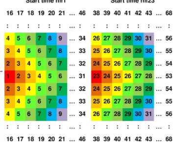
To get an idea of reasonable numbers for the statistical analysis of collocated along-track measurements with areal/temporal averaged estimates, simulations of in situ observation data sets and corresponding areal averages have been estimated from 8 min time series of precipitation measurements performed on the main building of the GEOMAR in Kiel, Germany. To derive simulated areal averages from a time series, the scheme given in Fig. 2 has been used based on the assumption that Taylor’s principle of frozen turbulence can be applied to precipitation fields in a similar manner, assuming a speed of motion of 5 m s⁻¹of precipitating clouds.

Thus, an 8 min interval is equivalent to a displacement of precipitating clouds by 2400 m. Areal averagesRfieldhave been computed according to

Rfield=

nmax

X

n=1

w(n)Rtimeseries(n), (1)

wherenindicates thenth element of the time series,w(n)is a weighting function according to the number of same elements of the time seriesR_timeseries(n)at a certain timenused

(5)

Figure 2. Scheme for estimates of simulated precipitation fields from precipitation time series gained on the main building of the GEOMAR in Kiel (54.3^◦N, 10.2^◦E) at a time interval of 8 min. The numbers, additionally highlighted by colours, indicate thenth 8 min interval of the time series. Assuming a speed of motion of precipitating clouds of 5 m s⁻¹, each 8 min interval is equivalent to a displacement of 2.4 km. Thus, a spatial field of 75 km×75 km is simulated by 31 elements×31 elements of the 8 min time series. Since ERA- Interim precipitation is accumulated over 3 h, simulated data have to be averaged over 23 consecutive fields (23×8 min=184 min).

Left: scheme for a spatial field representing ERA-Interim resolution at the beginning of a 184 min period, right at the end of this period. Start elements are indicated by red. The X indicates an observation, which is taken randomly from elementsn=1 ton=68 of the time series for ERA-Interim simulations and from elements n= −5 ton=37 for HOAPS simulations due to collocation criteria (Sects. 3.1 and 3.2).

for averaging, normalized by the total number of values used for averaging. Simulated in situ measurements were taken randomly from the same time series. With respect to the different resolutions of HOAPS and ERA-Interim and the assumed displacement of 2.4 km within any 8 min interval, we used a 21×21 field(21×8×60 s×5 m s⁻¹=50.4 km)for HOAPS averaging and a 31×31 field for ERA-Interim averaging.(31×8×60 s×5 m s⁻¹=74.4 km). While for HOAPS a simulated field was estimated at a certain starting time, simulated fields for ERA-Interim were estimated as an average over 23 consecutive fields in time (23×8 min=184 min), each constructed according to Fig. 2, to simulate the time increment of 3 h. Starting with element n=1 this gives nmax=31 for simulated fields of HOAPS andnmax=68 for simulated ERA-Interim fields. For HOAPS simulations, simulated point measurements were taken from those elements of the time series, which are within the temporal threshold used for collocation (see Sect. 3.1), and for ERA- Interim simulated measurements were taken from all mem- bers of the time series used for calculating the simulated

Figure 3.Examples of collocated data, which have been merged to events for HOAPS (top) and ERA-Interim (bottom). HOAPS’

footprints are indicated by the large circles, observations by◦, and ERA-Interim grid points by•. Colours indicate the rain rates, R.

HOAPS data are from day 338 in 1995, min 1272; collocated observations are from min 1235 to 1315. In the case of ERA-Interim, estimates are from day 338, min 1260 and 1440; collocated observations are from day 338, min 1227 to 1315.

fields. In the case of HOAPS, simulated fields with a precipitation rate below 0.3 mm h⁻¹are set to zero, according to the lower threshold in the HOAPS data.

3 Method

The statistical analysis follows the recommendations given by the WMO (World Meteorological Organization) for binary or dichotomous estimates (WWRP/WGNE, 2014).

Therefore it is necessary to collocate the data. In this study precipitation data from 1995–1997, gained over the Atlantic Ocean and the tropical Pacific Ocean, and 2005–2008, gained mainly over the Atlantic Ocean, together yield a point-to-area collocation against the satellite-derived climatology HOAPS and ERA-Interim reanalysis data.

(6)

3.1 Collocation HOAPS

As in a similar validation study over the Baltic Sea (Bumke et al., 2012), the nearest neighbour approach was chosen for collocation. Therefore, it must be ensured that both observations are related to each other, which can be determined by an appropriate decorrelation length. Decorrelation lengths had been derived from in situ precipitation data over the Baltic Sea: 17 km based on disdrometer 8 min time series (Bumke et al., 2012), 25 km for convective precipitation and 46–68 km for stratiform/frontal precipitation, based on 8 min time series of SRG measurements (Clemens and Bumke, 2002) on board merchant ships. Using 46 km as the decorrelation length for stratiform/frontal precipitation, these three numbers give an average decorrelation length of about 30 km which agrees well with a study of Puca et al. (2014). A decorrelation length of 30 km corresponds to a temporal correlation length of 45 min, assuming a merchant ship’s speed to be of the order of 20 Kn. Therefore, for the HOAPS collocation the allowed time difference was set to 45 min and the allowed distance was set to 55 km between the ship’s position and the satellite’s footprint (radius of the SSM/I pixel size plus decorrelation length). These match-up criteria are comparable to allowed differences of 45 min and 50 km chosen in a study by Klepp et al. (2010). According to the satellites’

overpass time, collocated data are merged to single events.

These last up to 90 min due to the match-up criteria; spatial extension varies according to the satellites’ footprints and ships’ positions and speeds (Fig. 3).

3.2 Collocation ERA-Interim

Our first requisite is that the time of the measurement is within the time interval of 3 h used for accumulation of the predicted precipitation. Furthermore, the four grid points, which enclose the ship’s position, were chosen. Again, collocated data are merged to single events, but now according to the time of the observations (1995–1997) or the time of the ERA-Interim products (2005–2008) taking the match-up criteria into account (Fig. 3).

4 Statistical analysis

In the following, the procedure chosen for validation of both HOAPS and ERA-Interim is presented. In total 654 events are available for the period from 1995 to 1997, which are split into 519 rain events and 135 snow events. A total of 2031 collocated rain-only events within the second period from 2005 to 2008 for HOAPS and 6011 for ERA-Interim are available. Each event has been checked as a function of a lower threshold, applied to measured precipitation rates, whether the measurements and reanalysis or satellite data give precipitation. Measured precipitation rates below that threshold were set to zero. If one or more measured precipitation rates of an event exceeded that threshold, the event was

flagged as “observed precipitation: yes”; if one of the satellite footprints or the ERA-Interim grid points of an event gives precipitation, independent of its precipitation rate, the event was flagged as “HOAPS or ERA-Interim precipitation: yes”.

Therefore, the threshold was set to 0.01 mm h⁻¹ for ERA- Interim and all smaller values were set to zero.

Following the recommendations given by the WMO (World Meteorological Organization) for binary or dichotomous estimates (WWRP/WGNE, 2014) 2×2 contingency tables are computed. They contain the hits (both HOAPS and measurements or both ERA-Interim and measurements give precipitation), the correct negatives (both HOAPS and measurements or both ERA-Interim and measurements give no precipitation), the misses (observation gives precipitation in contrast to HOAPS/ERA-Interim) and the false alarms (HOAPS/ERA-Interim gives precipitation in contrast to measurements).

This allows us to derive the accuracy, the bias score, the probability of detection (POD), the success ratio and the Hei- dke skill score. The accuracy is the fraction correct; 1 indicates perfect accuracy. It also depends on the number of correct negatives. The bias score answers the following question: how does the HOAPS/ERA-Interim frequency of “yes”

events compare to the observed frequency of “yes” events?

A score of 1 means that both data sets include the same number of precipitation events; a larger bias score indicates that there are more precipitation events in the HOAPS or ERA- Interim reanalysis data. The POD gives the proportion of measured precipitation events which can also be found in the HOAPS or ERA-Interim reanalysis data, with 1 indicating perfect agreement and 0 no agreement, while the success ratio gives the fraction of precipitation events in HOAPS or ERA-Interim reanalysis data that are also seen in measurements. Again, a score of 1 indicates perfect agreement, while 0 indicates maximum disagreement. It is equal to 1 minus the false alarm ratio, where the false alarm ratio gives the fraction of the observed no-events which were incorrectly fore- casted as yes. The Heidke skill score measures the fraction of correct estimates after eliminating those which would solely be correct by random chance. No skill is indicated by 0; a perfect score equals 1.

5 Results

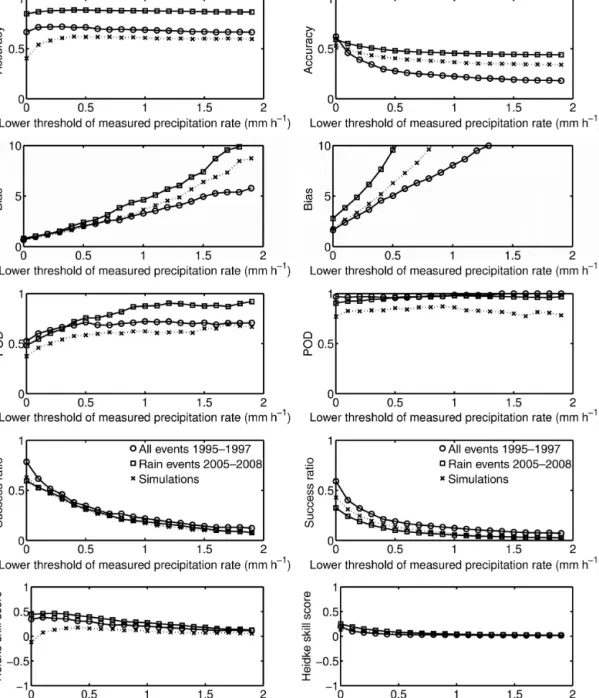
The results are given for the earlier period (1995–1997) in terms of accuracy, bias score, POD, success ratio and Heidke skill score as a function of an assumed lower threshold of measured precipitation rate (Fig. 4), below which the measured precipitation rates were set to zero. The statistical parameters are derived separately for rain events, snow events and all events; for comparison the results of the simulations (Sect. 2.5) are shown. The results for the 2006 to 2008 period are depicted in Fig. 5. The results derived from simulations (Sect. 2.5) and the rain-only events from the earlier

(7)

Figure 4.Accuracy, bias score, hit POD, success ratio and Heidke skill score (from top to bottom) against precipitation measurements for the period 1995–1997 (left HOAPS, right ERA-Interim) as a function of a lower threshold applied to the measurements.

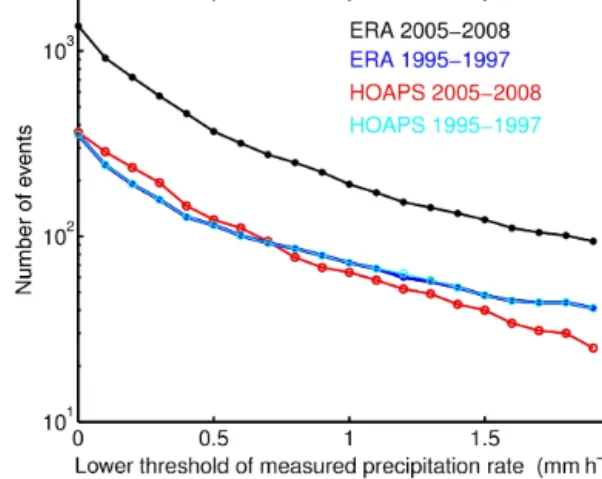
period (1995–1997) are shown for comparison. The numbers of events with measured precipitation are given in Fig. 6 as a function of the lower threshold for both periods and both collocated data sets. As expected numbers decrease rapidly with increasing threshold, since rain rate is distributed as a power law.

Taking into account that ERA-Interim data have no precipitation threshold, only rain rates below 0.01 mm h⁻¹ are set to zero for the statistical analysis. Best agreement is expected if no threshold is applied to the measurements. For

HOAPS, with a lower threshold of 0.3 mm h⁻¹, best results can be expected for a lower threshold in measurements similar to that of HOAPS. This is seen in the estimated accuracy, where HOAPS shows the best performance for measurement thresholds ranging between 0.1 and 0.5 mm h⁻¹, while ERA- Interim reaches highest values of accuracy when no threshold is applied to observational data. Obviously the performance of HOAPS to detect snow is lower compared to ERA- Interim (0.6 to 0.8), but it is still close to the results for simulated data; deviations are less than 0.04 in terms of accuracy

(8)

Figure 5.Accuracy, bias score, POD, success ratio and Heidke skill score (from top to bottom) against precipitation measurements for the period 2005–2008 (left HOAPS, right ERA-Interim) as a function of a lower threshold applied to the measurements.

for thresholds of 0.1 to 0.5 mm h⁻¹in measurements. On the other hand, estimated snow accuracies for ERA-Interim decrease rapidly for higher thresholds applied to the measurements. The rain performance of ERA-Interim is weaker than that of HOAPS in terms of accuracy, and for a wide range of thresholds applied to the measurements it is even lower than estimated for simulated fields. Note that the different behaviour of simulations with an increasing lower threshold in the measurements is due to the assumption of a lower threshold of 0.3 mm h⁻¹in the simulated fields for HOAPS.

The bias score, for which perfect agreement is given at value

1, indicates that ERA-Interim’s frequency of precipitation exceeds that of the measurements, strongly increasing with increasing threshold applied to measurements. HOAPS’ bias score is close to 1 for a lower threshold in the observation data ranging from 0.1 to 0.2 mm h⁻¹; the increase with increasing lower threshold applied to the measurements is less prominent. The results for the simulations indicate that this is mainly a result of averaging over larger areas due to the resolution of the ERA-Interim analysis, although the model description states that ERA-Interim grid point values do not represent an areal average (ECMWF, 2015).

(9)

It is obvious that the POD (Fig. 4) should increase with the lower threshold in measurements, because intense measured precipitation events should be easier to detect than low intensity precipitation events. PODs for HOAPS are of the order of 0.5 to 0.7; the smallest values are estimated for solid precipitation. Nevertheless, the values of simulations indicate a good agreement between HOAPS and the measurements.

The ERA-Interim precipitation estimates show PODs close to 1, not depending on a lower threshold applied to measured data. These high PODs mainly originate from the high values of the bias score; i.e. when ERA-Interim frequently gives precipitation it also shows precipitation in more or less all cases where precipitation was measured. The POD numbers derived from simulations also indicate that this might be par- tially a result of the coarser spatial resolution.

The success ratios show reasonable results for both data sets. Success ratios for HOAPS compared to measurements reach values of 0.7 to 0.9 for the lowest threshold applied to the measurements and decrease with increasing lower threshold, as expected. These numbers are comparable to those of the PODs and again indicate a good agreement between HOAPS and measurements. Values are a little higher than those estimated from simulations, and differences between different kinds of precipitation are small again. The success ratios of ERA-Interim reanalysis data compared to measurements are much smaller, which is a consequence of the high frequency of precipitation events in the ERA-Interim reanalysis data as also reflected in the bias score; i.e. when ERA- Interim estimates that the frequency of precipitation is too high, precipitation is also not measured in all cases. The Hei- dke skill score is in general higher for HOAPS than ERA- Interim, indicating a better performance of HOAPS in detecting precipitation with slight weaknesses in the case of snow.

As expected the Heidke skill score decreases with increasing lower threshold applied to the measurements. Nevertheless, a comparison to the results for the simulations also depicts a good performance of the ERA-Interim reanalysis data in cor- rectly predicting the occurrence of precipitation events, taking into account the coarser resolution of the ERA-Interim reanalysis data. Overall, validation results for solid and liquid precipitation show a similar level of detection for rain and snow.

Figure 5 gives the results for the second period, 2005 to 2008. For comparison the results for the period 1995 to 1997, as well as for the simulations are also provided. Since the frequency of events with no precipitation has increased compared to the earlier period, because instruments were running continuously (Sect. 2), accuracies have enhanced considerably, but ERA-Interim still gives a less accurate estimate than HOAPS. This is mainly due to an increasing frequency of precipitation events in ERA-Interim, as indicated also by the bias score, which indicates that the frequency of precipitation in ERA-Interim data is about 3 times higher than in the measurements and also considerably exceeds the simulated bias score. This is in line with the estimated PODs, which

Figure 6.Number of events with measured precipitation, where the precipitation rates exceed the given lower threshold.

are again close to 1. The values of the success ratios for HOAPS are close to the estimates of the first period, while ERA-Interim gives success ratio numbers that are only about half the values of the earlier periods. The Heidke skill scores are in general slightly higher, but still remain on a low level, especially for ERA-Interim. In summary, HOAPS performs similarly during both periods, while ERA-Interim performs better in the earlier period.

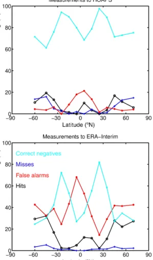
Since SRG and ODM 470 have a very similar performance for measuring and detecting rain (Fig. 1), the main difference between both periods might be caused by the coupling of the SRG and ODM 470 with a rain sensor during the first period. Thus, during the first period, all collocated data are from areas where precipitation is more likely due to the coupling of the instruments with a rain sensor, while during the second period, observational data might also cover areas where precipitation probability is low. To check whether this can explain the differences in the statistical parameters, Fig. 7 shows the location of data for both periods separately for HOAPS and ERA-Interim, indicating positions of misses, hits, false alarms and correct negatives. As can be seen from Fig. 7, for the period 1995 to 1997, there are al- most no data from the low-precipitation subtropical areas, although e.g. several Atlantic transits of R/VPolarsternare part of the database. This is also in contrast to the data distribution shown for the period 2005 to 2008. Please note in this context that the number of collocated events for ERA- Interim is considerably larger than for HOAPS in 2005 to 2008 as mentioned above. Comparing the number of false alarms (red) and the number of misses (blue) for HOAPS and ERA-Interim, it is obvious that ERA-Interim more frequently gives false alarms compared to HOAPS, while the frequency of misses is very low compared to HOAPS, as supported by estimated bias scores, PODs and success ratios. Largest differences are found in the area south of the equator and, less prominently, north of the intertropical convergence zone. Note that Fig. 8 gives the percentage of hits,

(10)

Figure 7.Location of collocated events (left: HOAPS and measurements, right: ERA-Interim and measurements) for the period 1995–1997 (top) and 2005–2008 (bottom). The different coloured symbols indicate misses, hits, false alarms and correct negatives. A lower threshold is not set.

misses, false alarms and correct negatives as a function of latitude belts. The most obvious feature is that ERA-Interim gives a much higher number of false alarms and a much lower number of correct negatives. This is supported by a strong increase of the bias score (Fig. 8), which shows a distinct maximum south of the equator, where ERA-Interim gives 15 times more rain than measured in terms of frequency, although the absolute number is relatively small, and a small maximum exists at 10–20^◦N, where ERA-Interim gives about 5 times more frequent rain than observed. The bias score of HOAPS also indicates an overestimation of the frequency of precipitation in the subtropics and tropics, but it is less striking. The latter can also be seen in the context of the number of available events, which are low in the area from 30^◦S to 10^◦N (Fig. 9).

Not shown are the results for the Heidke skill score, which gives the skill of a prediction with respect to a random prediction. The Heidke skill score shows values very close to 0 in the areas between 30^◦S and the equator for ERA-Interim and between 10^◦S and the equator and 20 to 30^◦N for HOAPS, indicating poor skill of both data sets in these areas compared to observed precipitation, which is also reflected in Figs. 8

and 9. This is also mainly caused by the very small number of observed precipitation events in these areas.

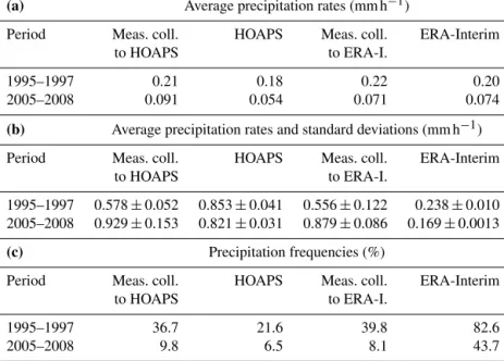
Although the comparison of along-track measurements with areal and temporal averages does not allow precipitation rates to be directly compared, the number of events in the first period (657 for HOAPS and ERA-Interim) and in the second period (2031 for HOAPS and 6011 for ERA-Interim), the latter also including more events with no precipitation, allows for a first comparison of average precipitation rates (Table 1a and b).

In the earlier period, where precipitation is more likely, HOAPS underestimates observed precipitation by 15 % and ERA-Interim by less than 10 %. For the 2005–2008 period, HOAPS underestimates precipitation considerably by 40 %, while ERA-Interim performs much better with a slight overestimation of only 4 % (Table 1a).

Using collocated data pairs instead of precipitation events and restricting the analysis to non-zero precipitation data, the number of data is sufficient to estimate the standard deviation by applying the bootstrap method (Efron, 1979). For the 1995–1997 period HOAPS shows on average significantly higher precipitation rates and ERA-Interim shows signifi-

(11)

Figure 8.Hits, misses, false alarms and correct negatives of events for the period from 2005 to 2008 as a function of latitude (latitude belts are south of 50, 50–40, 40–30, 30–20, 20–10 and 10–0^◦S;

0–10, 10–20, 20–30, 30–40, 40–50, 50–60 and north of 60^◦N) for HOAPS (top) and ERA-Interim (bottom). A lower threshold is not set for ERA-Interim data.

cantly lower precipitation rates than observed (Table 1b).

These differences in precipitation rates were in part balanced by precipitation frequency, which is lower for HOAPS and considerably higher for ERA-Interim than observed. For the 2005–2008 period ERA-Interim again shows significantly lower precipitation rates than observed, while HOAPS com- pares well with observations; the deviation is within 1 standard deviation. However, the deficit in the average precipitation rate of ERA-Interim goes along with an extreme overestimation of precipitation frequency of more than 400 %, while HOAPS shows an underestimation of precipitation frequency by about one third (Table 1b and c).

In summary, ERA-Interim overestimates the frequency of precipitation considerably, but combined with low precipitation rates, the mean precipitation is close to measurements. In contrast, HOAPS underestimates the frequency of precipitation, but even the higher average precipitation rate of HOAPS cannot balance the deficit compared to measurements. For

Figure 9.Bias score (top) and number of events (bottom) for the period 2005–2008 as a function of latitude (latitude belts are south of 50, 50–40, 40–30, 30–20, 20–10 and 10–0^◦S; 0–10, 10–20, 20–

30, 30–40, 40–50, 50–60 and north of 60^◦N) for HOAPS and ERA- Interim. A lower threshold is not set for ERA-Interim data.

the period 2005–2008, average precipitation rates are also given as a function of latitude for collocated data of measurements and ERA-Interim products (Fig. 10). The main features are a slight underestimation in the mid-latitudes of both hemispheres, a strong overestimation in the southern subtropics and the area of the intertropical convergence zone and an overestimation in high northern latitudes. Standard deviations were again estimated by applying the bootstrap method (Efron, 1979) to take into account that precipitation is not Gaussian-distributed. They are generally small for ERA-Interim, much smaller than for measurements. Es- timates from simulated measurements and fields, both with mean values of 0.19 mm h⁻¹, also give smaller standard deviations for the fields (0.028 mm h⁻¹) compared to measurements (0.063 mm h⁻¹), but differences are not as large. This possibly indicates too little variability in the ERA-Interim precipitation rates. The relatively small number of collocated HOAPS data does not allow for a comparison of precipitation rates with measurements for all latitudinal belts; however, north of 40^◦N and south of 30^◦S (2005–2008) HOAPS

(12)

Table 1. Average precipitation rates (mm h⁻¹) of precipitation events(a)and average precipitation rates and their standard deviation (mm h⁻¹) for all collocated data pairs restricted to non-zero precipitation data(b)for collocated measurements and collocated HOAPS respective ERA-Interim data. In(c), the precipitation frequencies ( %) derived from all collocated data pairs of both data sets are shown.

(a) Average precipitation rates (mm h⁻¹)

Period Meas. coll. HOAPS Meas. coll. ERA-Interim

to HOAPS to ERA-I.

1995–1997 0.21 0.18 0.22 0.20

2005–2008 0.091 0.054 0.071 0.074

(b) Average precipitation rates and standard deviations (mm h⁻¹)

to HOAPS to ERA-I.

1995–1997 0.578±0.052 0.853±0.041 0.556±0.122 0.238±0.010 2005–2008 0.929±0.153 0.821±0.031 0.879±0.086 0.169±0.0013

(c) Precipitation frequencies (%)

to HOAPS to ERA-I.

1995–1997 36.7 21.6 39.8 82.6

2005–2008 9.8 6.5 8.1 43.7

Figure 10.Mean precipitation rates of collocated data pairs for the period from 2005 to 2008 as a function of latitude (latitude belts are south of 50, 50–40, 40–30, 30–20, 20–10 and 10–0^◦S; 0–10, 10–20, 20–30, 30–40, 40–50, 50–60 and north of 60^◦N) for ERA-Interim compared to collocated measurements. Vertical bars indicate standard deviation estimated by applying the bootstrap method (Efron, 1979). A lower threshold is not set for ERA-Interim data.

underestimates mean precipitation rates considerably, with a total underestimation of about 40 %, as mentioned above.

6 Discussion

The main problem in interpreting the results is caused by a comparison of along-track point measurements with in-

stantaneous areal estimates (HOAPS) or estimates integrated over time (ERA-Interim). Moreover, the strong spatial and temporal variability and intermittency of the precipitation further complicates the validation efforts. Thus, we cannot expect a perfect agreement between the different data sets with respect to statistical parameters. To reduce this problem the data have been merged to events (see Fig. 3). In the case of HOAPS each event comprises on average 100 pairs of collocated data, in the case of ERA-Interim, 29 pairs of collocated data for the 1995–1997 period and 69 for the 2005–2008 period. To obtain an idea of reasonable statistical numbers, simulations of point-to-area collocations have been constructed. Comparisons of estimated statistical parameters resulting from these simulated collocations take into account, for example, that HOAPS data apply a lower precipitation threshold and that ERA-Interim data have a coarser spatial resolution.

Summarized statistical parameters, compared to the results for simulations of point-to-area collocation, show a reasonable ability of HOAPS to detect precipitation. However, the results also show that HOAPS underestimates the frequency of precipitation in the mid-latitudes and high latitudes, which is partly related to the threshold used in the HOAPS data.

This leads to an underestimation in the mean precipitation rate of up to 40 %, where the lower threshold in HOAPS may contribute only about 10 %, based on statistics from northern Germany. The ability to detect solid precipitation is a little weaker than for rain, but the derived statistical parameters are still comparable with simulations.

(13)

ERA-Interim performs well in areas where precipitation is more likely, especially for snow. Although the bias score is of order 2, it is still of the same order as the simulated data.

But the high values of the POD, not depending on a lower threshold of measurements, indicate that ERA-Interim overestimates the frequency of precipitation. This is more distinct in the period 2005 to 2008 and is extreme in the subtropical areas. For this period, statistical parameters reveal weaknesses in the ability of ERA-Interim to give correct precipitation estimates. Nevertheless averaged precipitation rates are close to the measured ones, with biases between −10 and +4 % when averaging over all areas. Looking at average precipitation rates for certain areas of the Atlantic Ocean reveals weaknesses. Although the statistics are uncertain in the subtropics, where the number of observed precipitation events is very low, results indicate that HOAPS and especially ERA- Interim overestimate the frequency of precipitation in these areas. For the area of the intertropical convergence zone, both HOAPS and ERA-Interim show precipitation rates that are too frequent. While it is not possible to estimate mean precipitation rates in the tropics and subtropics due to the low number of observed precipitation events for HOAPS, mean ERA- Interim precipitation rates are higher than observed ones in the inner tropics. While HOAPS generally underestimates precipitation rates north of 40^◦N and south of 30^◦S (period from 2005 to 2008), ERA-Interim underestimates precipitation south of 30^◦S and for latitudes between 40 and 50^◦N and overestimates it north of 50^◦N.

With respect to solid precipitation, although not reaching the high accuracy (96 %) as in a study of Klepp et al. (2010) between point-to-area collocations of ship-based ODM 470s and HOAPS data, the detectability of solid precipitation in terms of the success ratio shows a good performance in detecting snowfall by both HOAPS and ERA-Interim.

7 Summary and outlook

In this study HOAPS precipitation estimates and ERA- Interim precipitation estimates have been compared to in situ SRG and ODM 470 precipitation measurements on board a number of research vessels. The main features are an underestimation in intensity of precipitation by HOAPS, although results have shown that HOAPS performs well in detecting the frequency of precipitation. The frequency of precipitation is strongly overestimated by ERA-Interim, especially in the tropics and subtropics. The Atlantic-wide average precipitation rate is close to measurements, but a distinct feature is an overestimation in the area of the intertropical convergence zone.

These results have to be put into context with evaporation in order to make estimates of the freshwater flux, which influ- ences salinity and is one of the key parameters in ocean mod- elling. The overestimation of precipitation by ERA-Interim might be balanced with respect to the freshwater budget by

an overestimation of ERA-Interim evaporation in the tropics (Kinzel, 2013), but in higher latitudes it is not the case.

Additionally, the underestimation in HOAPS precipitation is associated with an underestimation of HOAPS evaporation (Kinzel, 2013); thus, errors in the freshwater budget are also expected to be small.

Therefore, in the course of 2017, when HOAPS 4 data are also available for 2008 onwards, an extended time period will be used to enhance the validation study for precipitation and to also include evaporation in order to make direct estimates of the freshwater flux. In this context, it also has to be pointed out that the other main problem in validating precipitation over the sea (beside the problem comparing point measurements with areal estimates) is the paucity of accurate precipitation measurements over the sea. Extending the investigation for the time after 2008 will make the results more robust against single events. It is also planned, in co- operation with OceanRAIN (Klepp, 2015), to use another set of precipitation data gained by ODM 470s mounted on nine research vessels worldwide. These data also cover the period after 2008 and will give the validation a broader basis.

Data availability

Meteorological data of R/VMaria S. Merianare provided from the DOD (Deutsches Ozeanographisches Datenzen- trum) maintained by the Bundesamt für Seeschifffahrt und Hydrographie (2015). Information for the meteorological data (2005–2008) and observatory of R/VPolarsterncan be found in König-Langlo et al. (2006). Precipitation measurements of the 1995–1997 period, measurements on R/VAlkor and on the GEOMAR building in Kiel are archived in the Pangaea data library (Bumke et al., 2016). ERA-Interim data (Dee et al., 2011) are accessible via the ECMWF data server.

Acknowledgements. We would especially like to thank the captains and their crews for supporting the precipitation measurements on board all research vessels. Meteorological data of R/VMaria S.

Merianare provided from the DOD (Deutsches Ozeanographisches Datenzentrum) maintained by the Bundesamt für Seeschifffahrt und Hydrographie.

Special thanks go to Reimer Wolf from the Briese Research ship- ping agency for his engagement in performing precipitation measurements on R/VMaria S. Merian. We would like to express our warm thanks to Lutz Hasse posthumously, who initiated the precipitation measurements over the sea, and his former working group in Kiel. ERA-Interim data used in this study were obtained from the ECMWF data server. Our thanks also go to Christian Klepp and to Lisa Neef for proofreading.

Further, we would like to thank the editor and especially the anonymous reviewers for their constructive comments and suggestions that helped to improve our manuscript.

The article processing charges for this open-access publication were covered by a Research

Centre of the Helmholtz Association.

(14)

Edited by: M. Kulie

References

Adler, R. F., Huffman, G. J., Chang, A., Ferraro, R., Xie, P.-P., Janowiak, J., Rudolf, B., Schneider, U., Curtis, S., Bolvin, D., Gruber, A., Susskind, J., Arkin, P., and Nelkin, E.: The Version-2 Global Precipitation Climatology Project (GPCP) Monthly Pre- cipitation Analysis (1979–Present), J. Hydrometeorol., 4, 1147–

1167, 2003.

Andersson, A., Fennig, K., Klepp, C., Bakan, S., Graßl, H., and Schulz, J.: The Hamburg Ocean Atmosphere Parameters and Fluxes from Satellite Data – HOAPS-3, Earth Syst. Sci. Data, 2, 215–234, doi:10.5194/essd-2-215-2010, 2010.

Andersson, A., Klepp, C., Fennig, K., Bakan, S., Graßl, H., and Schulz, J.: Evaluation of HOAPS-3 ocean surface freshwater flux components, J. Appl. Meteorol. Climatol., 50, 379–398, doi:10.1175/2010JAMC2341.1, 2011.

Behrangi, A., Hsu, K.-L., Iman, B., Sorooshian, S., Huffman, G.

J., and Kulikowski, R. J.: PERSIANN-MSA: A precipitation estimation method from satellite-based multispectral analysis, J.

Hydrometeorol., 10, 1414–1429, doi:10.1175/2009JHM1139.1, 2009.

Belo-Pereira, M., Dutra, E., and Viterbo, P.: Evaluation of global precipitation data sets over the Iberian Peninsula, J. Geophys.

Res., 116, D20101, doi:10.1029/2010JD015481, 2011.

Berrisford, P., Kållberg, P., Kobayashi, S., Dee, D., Uppala, S., Sim- mons, A. J., Poli, P., and Sato, H.: Atmospheric conservation properties in ERA-Interim, Q. J. Roy. Meteor. Soc., 137, 1381–

1399, doi:10.1002/qj.864, 2011.

Brandes, E. A., Ikeda, K., Zhang, G., Schönhuber, M., and Ras- mussen, R. M.: A statistical and physical description of hydrom- eteor distributions in Colorado snowstorms using a video disdrometer, J. Appl. Met. Clim., 46, 634–650, 2007

Bumke, K., Clemens, M., Grassl, H., Pang, S., Peters, G., Seltmann, J. E. E., Siebenborn, T., and Wagner, A.: Accurate areal precipitation measurements over the land and sea (APOLAS), BALTEX Newsletter 6, 9–13, 2004.

Bumke, K., Fennig, K., Strehz, A., Mecking, R., and Schröder, M.: HOAPS precipitation validation with ship-borne rain gauge measurements over the Baltic Sea, Tellus A, 64, 18486, doi:10.3402/tellusa.v64i0.18486, 2012.

Bumke, K., König-Langlo, G., Kinzel, J., and Schröder, M.: Pre- cipitation over sea: Validation against shipboard in-situ measurements, doi:10.1594/PANGAEA.858657, last access: 27 May 2016.

Bundesamt für Seeschifffahrt und Hydrographie (BSH): DOD Data Centre, available at: http://www.bsh.de/en/Marine_data/

Observations/DOD_Data_Centre/ (last access: 27 May 2016), 2015.

Clemens, M.: Machbarkeitsstudie zur räumlichen Niederschlags- analyse aus Schiffsmessungen über der Ostsee, PhD thesis, Christian-Albrechts-Universität, Kiel, 178 pp., 2002

Clemens, M. and Bumke, K.: Precipitation fields over the Baltic Sea derived from ship rain gauge on merchant ships, Boreal Environ.

Res., 7, 425–436, 2002.

Dee, D. P., Uppala, S. M., Simmons, A. J., Berrisford, P., Poli, P., Kobayashi, S., Andrae, U., Balmaseda, M. A., Balsamo, G., Bauer, P., Bechtold, P., Beljaars, A. C. M., van de Berg, L., Bid- lot, J., Bormann, N., Delsol, C., Dragani, R., Fuentes, M., Geer, A. J., Haimberger, L., Healy, S. B., Hersbach, H., Hólm, E. V., Isaksen, L., Kållberg, P., Köhler, M., Matricardi, M., McNally, A. P., Monge-Sanz, B. M., Morcrette, J.-J., Park, B.-K., Peubey, C., de Rosnay, P., Tavolato, C., Thépaut, J.-N. and Vitart, F.: The ERA-Interim reanalysis: configuration and performance of the data assimilation system, Q. J. Roy. Meteor. Soc., 137, 553–597, 2011.

Durack, P. J., Wijffels, S. E., and Matear, R. J.: Ocean Salinities Reveal Strong Global Water Cycle Intensification During 1950 to 2000, Science, 336, 455–458, doi:10.1126/science.1212222, 2012.

ECMWF, FAQ: Over what horizontal area are grid point data values valid?, available at: http://www.ecmwf.int/en/

over-what-horizontal-area-are-grid-point-data-values-valid (last access: 27 May 2016), 2015.

Efron, B.: Bootstrap Methods: Another Look at the Jackknife, Ann.

Stat., 7, 1–26, doi:10.1214/aos/1176344552, 1979.

Froidurot, S., Zin, I., Hingray, B., and Gautheron, A.: Sensi- tivity of Precipitation Phase over the Swiss Alps to Differ- ent Meteorological Variables, J. Hydrometeorol., 15, 685–696, doi:10.1175/JHM-D-13-073.1, 2014.

Grist, J. P., Josey, S. A., Marsh, R., Kwon, Y.-O., Bingham, R. J., and Blaker, A. T.: The Surface-Forced Overturning of the North Atlantic: Estimates from Modern Era Atmospheric Reanalysis Datasets, J. Climate, 27, 3596–3618, doi:10.1175/JCLI-D-13- 00070.1, 2014.

Großklaus, M.: Niederschlagsmessung auf dem Ozean von fahren- den Schiffen, Dissertation, Institut für Meereskunde an der Christian-Albrechts-Universität Kiel, 1996.

Großklaus, M., Uhlig, K., and Hasse, L.: An optical disdrometer for use in high wind speeds, J. Atmos. Ocean. Technol., 15, 1051–

1059, 1998.

Hasse, L., Großklaus, M., Uhlig, K., and Timm, P.: A ship rain gauge for use under high wind speeds, J. Atmos. Ocean. Tech- nol., 15, 380–386, 1998.

Hogan, A.: Objective estimates of airborne snow properties, J. At- mos. Ocean. Technol., 11, 432–444, 1994.

Huffman, G. J., Adler, R. F., Arkin, P., Chang, A., Ferraro, R., Gru- ber, A., Janowiak, J., McNab, A., Rudolf, B., and Schneider, U.:

The Global Precipitation Climatology Project (GPCP) combined precipitation dataset, B. Am. Meteorol. Soc., 78, 5–20, 1997.

Huffman, G. J., Adler, R. F., Bolvin, D. T., Gu, G., Nelkin, E.

J., Bowman, K. P., Hong, Y., Stocker, E. F., and Wolff, D. B.:

The TRMM Multi-satellite Precipitation Analysis: Quasi-Global, Multi-Year, Combined-Sensor Precipitation Estimates at Fine Scale, J. Hydrometeorol., 8, 38–55, 2007.

Huffman, G. J., Bolvin, D. T., and Nelkin, E. J.: Integrated Multi- satellitE Retrievals for GPM (IMERG) Technical Documen- tation, NASA/GSFC Code 612, 47 pp., http://pmm.nasa.gov/

sites/default/files/document_files/IMERG_doc.pdf (last access:

27 May 2016), 2015.

Joyce, R. J., Janowiak, J. E., Arkin, P. A., and Xie, P.: CMORPH: A Method that Produces Global Precipitation Estimates from Pas- sive Microwave and Infrared Data at 8 km, Hourly Resolution, J.

Climate, 5, 487–503, 2004.

(15)

Kållberg, P.: Forecast drift in ERA-Interim, ERA report series no, 10, http://www.ecmwf.int/sites/default/files/elibrary/2011/

10381-forecast-drift-era-interim.pdf (last access: 27 May 2016), 2011.

Kidd, C., Dawkins, E., and Huffman, G. J.: Comparison of Precipitation Derived from the ECMWF Operational Forecast Model and Satellite Precipitation Datasets, J. Hydrometeorol., 14, 1463–1482 doi:10.1175/JHM-D-12-0182, 2013.

Kinzel, J.: Validation of HOAPS latent heat fluxes against parame- terizations applied to RVPolarsterndata for 1995–1997 (Master thesis), Christian-Albrechts-Universität Kiel, Kiel, Germany, 96 pp., 2013.

Klepp, C.: The Oceanic Shipboard Precipitation Measurement Net- work for Surface Validation – OceanRAIN, Atmos. Res., 163, 74–90, doi:10.1016/j.atmosres.2014.12.014, 2015.

Klepp C., Bumke, K., Bakan, S., and Bauer, P.: Ground validation of oceanic snowfall detection in satellite climatologies during LOFZY, Tellus A, 62, 469–480, doi:10.1111/j.1600- 0870.2010.00459.x, 2010.

König-Langlo, G., Loose, B., and Bräuer, B.: 25 Years of Po- larsternMeteorology, WDC-MARE Reports, 4 (CD-ROM), 1–

137, doi:10.2312/wdc-mare.2006.4, 2006.

Lempio, G., Bumke, K., and Macke, A.: Measurement of solid precipitation with an optical disdrometer, Adv. Geosci., 10, 91–97, 2007.

Lindsay, R., Wensnahan, M., Schweiger, A., and Zhang, J.: Eval- uation of Seven Different Atmospheric Reanalysis Products in the Arctic, J. Climate, 27, 2588–2606, doi:10.1175/JCLI-D-13- 00014.1, 2014.

Liu, C. and Allan, R. P.: Observed and simulated precipitation responses in wet and dry regions 1850–2100, IOP Pub- lishing Ltd, Environ. Res. Lett., 8, 11 pp., doi:10.1088/1748- 9326/8/3/034002, 2013.

Macke, A., Francis, P. N., Mc Farquhar, G. M., and Kinne, S.: The role of ice particle shapes and size distributions in the single scat- tering properties of cirrus clouds, J. Atmos. Sci., 55, 2874–2883, 1998.

Mugnai, A., Casella, D., Cattani, E., Dietrich, S., Laviola, S., Lev- izzani, V., Panegrossi, G., Petracca, M., Sanò, P., Di Paola, F., Biron, D., De Leonibus, L., Melfi, D., Rosci, P., Vocino, A., Zauli, F., Pagliara, P., Puca, S., Rinollo, A., Milani, L., Porcù, F., and Gattari, F.: Precipitation products from the hydrology SAF, Nat. Hazards Earth Syst. Sci., 13, 1959–1981, doi:10.5194/nhess-13-1959-2013, 2013.

O’orman, P. A., Allan, R. P., Byrne, M. P., and Previdi, M.: Ener- getic Constraints on Precipitation Under Climate Change, Surv.

Geophys., 33, 585–608, doi:10.1007/s10712-011-9159-6, 2012.

Pfeifroth, U., Mueller, R., and Ahrens, B.: Evaluation of Satellite- Based and Reanalysis Precipitation Data in the Tropical Pacific, J. Appl. Meteor. Climatol., 52, 634–644, doi:10.1175/JAMC-D- 12-049.1, 2013.

Puca, S., Porcu, F., Rinollo, A., Vulpiani, G., Baguis, P., Bala- banova, S., Campione, E., Ertürk, A., Gabellani, S., Iwanski, R., Jurašek, M., Kanák, J., Kerényi, J., Koshinchanov, G., Koz- inarova, G., Krahe, P., Lapeta, B., Lábó, E., Milani, L., Okon, L’., Öztopal, A., Pagliara, P., Pignone, F., Rachimow, C., Rebora, N., Roulin, E., Sönmez, I., Toniazzo, A., Biron, D., Casella, D., Cattani, E., Dietrich, S., Di Paola, F., Laviola, S., Levizzani, V., Melfi, D., Mugnai, A., Panegrossi, G., Petracca, M., Sanò, P., Za- uli, F., Rosci, P., De Leonibus, L., Agosta, E., and Gattari, F.: The validation service of the hydrological SAF geostationary and polar satellite precipitation products, Nat. Hazards Earth Syst. Sci., 14, 871–889, doi:10.5194/nhess-14-871-2014, 2014.

Rhein, M., Rintoul, S. R., Aoki, S., Campos, E., Chambers, D., Feely, R. A., Gulev, S., Johnson, G. C., Josey, S. A., Kos- tianoy, A., Mauritzen, C., Roemmich, D., Talley, L. D., and Wang, F.: Observations: Ocean, in: Climate Change 2013: The Physical Science Basis, Contribution of Working Group I to the Fifth Assessment Report of the Intergovernmental Panel on Cli- mate Change, edited by: Stocker, T. F., Qin, D., Plattner, G.- K., Tignor, M., Allen, S. K., Boschung, J., Nauels, A., Xia, Y., Bex, V., and Midgley, P. M., Cambridge University Press, Cam- bridge, United Kingdom and New York, NY, USA, 659–740, doi:10.1017/CBO9781107415324.018, 2013.

Schmitt, R. W.: Salinity and the global water cycle, Oceanography, 21, 12–19, doi:10.5670/oceanog.2008.63, 2008.

Thiemig, V., Rojas, R., Zambrano-Bigiarini, M., Levizzani, V., and De Roo, A.: Validation of Satellite-Based Precipitation Products over Sparsely Gauged African River Basins, J. Hydrometeorol., 13, 1760–1783, doi:10.1175/JHM-D-12-032.1, 2012.

Trenberth, K. E.: Changes in precipitation with climate change, Clim. Res., 47, 123–138, 2011.

Valdivieso, M. and Haines, K.: Scientific Validation Report (ScVR) for v1 Reprocessed Analysis and Reanalysis, GMES Marine Core Services Technical Report WP04-GLO-U-Reading_v1, 28 pp., March 2011, 2011.

Wang, J. J., Adler, R. F., Huffman, G. J., and Bolvin, D. F.: An Up- dated TRMM Composite Climatology of Tropical Rainfall and Its Validation, J. Climate, 27, 273–284, doi:10.1175/JCLI-D-13- 00331.1, 2014.

WWRP/WGNE.: Methods for dichotomous forecasts, Joint Working Group on Verification sponsored by the WMO, forecast verification, issues, methods and FAQ, available at: www.cawcr.gov.au/projects/verification/#Methods_for_

dichotomousforecasts (last access: 27 May 2016), 2014.