atmosphere
Article
Validation of ERA-Interim Precipitation Estimates over the Baltic Sea
Karl Bumke
GEOMAR Helmholtz Centre for Ocean Research Kiel, Düsternbrooker Weg 20, Kiel 24105, Germany;
kbumke@geomar.de; Tel.: +49-431-600-4060 Academic Editor: Katja Friedrich
Received: 20 May 2016; Accepted: 7 June 2016; Published: 11 June 2016
Abstract:European Centre for Medium-Range Weather Forecasts (ECMWF) ERA-Interim reanalysis total precipitation estimates are validated against ten years ofin situprecipitation measurements onboard of ships over the Baltic Sea. A statistical analysis for binary forecasts and mean rain rates derived from all data show a good agreement with observations. However, a closer look reveals an underestimation of ERA-Interim total precipitation in spring and an overestimation in autumn, obviously related to stability. Deriving stability and evaporation by a bulk flux scheme it could be shown, in fact, that ERA-Interim underestimates precipitation for conditions with low evaporation and strongly overestimates it for conditions with high evaporation. Since ERA-Interim surface fields become too dry with increasing evaporation compared to independent synoptic ship observations, uncertainties in the ECMWF convection scheme may possibly cause these biases in seasonal precipitation.
Keywords:precipitation; Baltic Sea; ERA-Interim; evaporation; ship rain gauge
1. Introduction
The Baltic Sea is a semi-enclosed sea, which is strongly influenced by human activities due to its location. Therefore, there is a need to investigate the functioning of the marine system, for which the energy and water cycles determine the boundary conditions. Several efforts have been undertaken within the BALTEX (BALTic Sea EXperiment) research program [1,2] to improve our understanding of these cycles and their interconnections. However, despite progress in Baltic Sea research, several gaps remain. For example, [1] found that changes in ocean salinity are not fully understood and modelling of the hydrological cycle in atmospheric climate models is severely biased. They, thus, concluded that more detailed investigations of regional precipitation and evaporation patterns are still needed.
The past decade has also seen great improvement in the creation of reanalysis datasets, which may serve as an additional source of information. However, [3] performed a comprehensive study of several reanalysis data sets including ERA-Interim [4] and found that the reanalyses produce quite good results for precipitation over land but, evaporation, precipitation, and their difference, are not stable over the ocean. He suggested that these data probably should only be used if their validity can be demonstrated. This is difficult, mainly due to the lack of ground-based measurements over the sea. Thus, most precipitation estimates are based on algorithms applied to satellite data, like GPCP (Global Precipitation Climatology Project) [5,6], the Hamburg Ocean Atmosphere Parameters and Fluxes from Satellite data [7,8], or IMERG (Integrated Multi-satellitE Retrievals for Global precipitation measurement [9]) to mention a few. However, concerns have been expressed over the need for further work to evaluate these data sets [10]. This is supported by a study of [8], who pointed out that state-of-the-art satellite retrievals and reanalysis datasets still disagree on global precipitation amounts, patterns, variability, and temporal behavior, with the relative differences increasing poleward. Several
Atmosphere2016,7, 82; doi:10.3390/atmos7060082 www.mdpi.com/journal/atmosphere
studies have also shown that ERA-Interim overestimates especially the frequency of rain events, see e.g., [11] or [12].
Most of the validation studies compared data to measurements on small islands or atolls, although the representativeness of these measurements for open-ocean rainfall is still an open question [13].
To overcome this problem, the present validation study of ERA-Interim precipitation over the Baltic Sea only usein situmeasurements of precipitation by ship rain gauges for a ten year period from 1995 to 2004.
2. Data
2.1. Ship Rain Gauge Measurements
The ship rain gauge [14] is commercially available from Eigenbrodt Environmental Measurement Systems near Hamburg, Germany. An outstanding feature of the ship rain gauge is an additional lateral collector, which is especially effective under high wind speed conditions. Both collectors are separately connected to drop forming devices. This allows the derivation of precipitation rates together with measured relative wind speed. Details of the algorithm are given in [15]. Comparisons to other instruments show that the ship rain gauge performs well and gives nearly unbiased estimates of rainfall [16]. Simultaneous measurements of a ship rain gauge and an optical disdrometer onboard the R/V Alkor over the Baltic Sea also emphasize the ability of the ship rain gauge to accurately measure rain rates [17].
Ship rain gauges have been mounted on a number of research vessels and merchant ships. The position and time at the end of each measurement interval were taken from additional GPS (Global Positioning System) information. Measurement intervals were 8 min on most ships; only R/V Alkor has original measurement intervals of 1 min, which were integrated over 8 min for validation purposes.
Figure1shows measurement periods of each ship used in this study, which span in total the period from 1995 to 2004. Since ship rain gauges are not suitable to measure snow, only data collected at air temperatures above 4˝C [18] have been used. Since air temperatures were not measured on all ships, they are taken from the collocated ERA-Interim product.
Atmosphere 2016, 7, 82 2 of 13
poleward. Several studies have also shown that ERA-Interim overestimates especially the frequency of rain events, see e.g., [11] or [12].
Most of the validation studies compared data to measurements on small islands or atolls, although the representativeness of these measurements for open-ocean rainfall is still an open question [13]. To overcome this problem, the present validation study of ERA-Interim precipitation over the Baltic Sea only use in situ measurements of precipitation by ship rain gauges for a ten year period from 1995 to 2004.
2. Data
2.1. Ship Rain Gauge Measurements
The ship rain gauge [14] is commercially available from Eigenbrodt Environmental Measurement Systems near Hamburg, Germany. An outstanding feature of the ship rain gauge is an additional lateral collector, which is especially effective under high wind speed conditions. Both collectors are separately connected to drop forming devices. This allows the derivation of precipitation rates together with measured relative wind speed. Details of the algorithm are given in [15]. Comparisons to other instruments show that the ship rain gauge performs well and gives nearly unbiased estimates of rainfall [16]. Simultaneous measurements of a ship rain gauge and an optical disdrometer onboard the R/V Alkor over the Baltic Sea also emphasize the ability of the ship rain gauge to accurately measure rain rates [17].
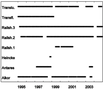
Ship rain gauges have been mounted on a number of research vessels and merchant ships. The position and time at the end of each measurement interval were taken from additional GPS (Global Positioning System) information. Measurement intervals were 8 min on most ships; only R/V Alkor has original measurement intervals of 1 min, which were integrated over 8 min for validation purposes. Figure 1 shows measurement periods of each ship used in this study, which span in total the period from 1995 to 2004. Since ship rain gauges are not suitable to measure snow, only data collected at air temperatures above 4 °C [18] have been used. Since air temperatures were not measured on all ships, they are taken from the collocated ERA-Interim product.
Figure 1. Ships and periods of measurements. Translubeca, Transfinlandia, Railship 1, 2, and 3, and Antares are merchant ships, Heincke and Alkor are research vessels.
2.2. ERA-Interim Reanalysis Precipitation Data
Precipitation data are provided in the ERA-Interim reanalysis [4]. Here, short-range forecast data are used as recommended by [19], constituting the final part of the ECMWF reanalysis compilation loop, which is produced with the Integrated Forecasting System [4] and comprises a forecast model
Figure 1.Ships and periods of measurements. Translubeca, Transfinlandia, Railship 1, 2, and 3, and Antares are merchant ships, Heincke and Alkor are research vessels.
2.2. ERA-Interim Reanalysis Precipitation Data
Precipitation data are provided in the ERA-Interim reanalysis [4]. Here, short-range forecast data are used as recommended by [19], constituting the final part of the ECMWF reanalysis compilation
Atmosphere2016,7, 82 3 of 13
loop, which is produced with the Integrated Forecasting System [4] and comprises a forecast model with three fully-coupled components representing the atmosphere, the land surface, as well as ocean waves. The atmospheric forecast model used for ERA-Interim has a 30 min time step and a spectral T255 horizontal resolution, which corresponds to roughly uniform 79 km spacing for surface- and other grid point fields [20]. For validation purposes total precipitation data have been extracted from the open-access ECMWF Data Server, as well as the land sea mask. Data consist of three hourly surface forecast fields from January 1995 to December 2004, which are initiated at 00 UTC and 12 UTC. The forecast data’s temporal resolution is twice as large as that of the surface analysis fields, which makes it attractive for validation studies. The ERA-Interim data used within this work are grid point values, meaning that they are not averaged area-wise but are rather valid at the exact location of the grid points [21]. Forecasted total precipitation data are given in the form of accumulated fields. To obtain the average between two time steps, the grid point-wise difference of both single fields was retrieved and multiplied by the inverse of the time step.
2.3. Supplementary Data ERA-Interim
Three hourly estimates of air temperature, dew point temperature, sea surface temperature, air pressure, wind speed, and instantaneous evaporation were downloaded from the ECMWF server as supplementary data. These data are also short-range forecast data due to their high temporal resolution.
They are used to analyze the meteorological conditions in terms of stability and evaporation, which may influence the precipitation forecast [22]. Stability was derived by applying two bulk parameterization schemes [23,24]. Furthermore, ERA-Interim 2 m temperatures were used to eliminate measurements of solid precipitation, as mentioned above.
2.4. Supplementary Marine Meteorological Data
To ensure that estimates of stability or evaporation are not biased due to biases in the ERA-Interim reanalysis data, we use high-quality ship observations as an additional source of information. These are hourlyin situdata, which originate from the marine meteorological data archive of the German Meteorological Service (DWD), supervised by the Seewetteramt Hamburg (SWA).
These are measurements in hourly resolution. We extracted air pressure p, air temperature T, dew point temperature Td, sea surface temperature SST, and wind speed u data to estimate stability and latent heat flux independently of the ERA-Interim data. A stability-dependent height correction was applied to air temperature, specific humidity, and wind speed using a bulk flux scheme [23]. Since individual measurement heights are not available in the data, we assume an average measurement height of 18 m [25].
2.5. Weather Radar Data
Rostock weather radar data are used to simulate ERA-Interim grid points and collocated ship observations. It is located directly at the southern coast of the Baltic Sea (54˝101351 1N, 12˝031331 1E). For the simulations the lowest volume scan, with a range resolution of 1 km and a beam width of 1˝, was used. The inclination is 0.5˝and temporal resolution 15 min. The radar has a range of 128 km working in Doppler mode. Approximately one year of data is available from 2002 and 2003.
3. Method
3.1. Collocation
Our first requisite for collocation is that the time of the observation is within the 3 h forecast interval, which is the time interval used for accumulation of the precipitation. Furthermore, observations were collocated with the four grid points which enclose the ship’s position. Therefore, the maximum distance between a collocated measurement and a gridpoint is about 95 km at the most southern part of the Baltic Sea, which agrees well with findings of typical precipitation decorrelation
lengths of 100 km for a 3 h time interval [26]. Collocated data are merged into single events for each grid point and time, excluding ERA-Interim data over land. Thus, these events last up to 3 h. On average 15 to 16 measurements, each of a duration of 8 min, were collocated to a single grid point.
Thus, the observed precipitation rate represents an average over these observations, or about 2 h of data on average. The decorrelation length for this time interval is about 90 km [26], which is also of the order of the maximum distance chosen for collocation.
The SWA marine data were also collocated with the four surrounding grid points, but here the maximum temporal difference is set to 2 h following [27].
3.2. Stability and Latent Heat Fluxes
Stability, expressed in terms of the Monin-Obukhov stability parameter [28], and latent heat fluxes were derived from air temperature, humidity, wind speed, air pressure, and SST by applying a bulk scheme [23]. Input parameters are taken from observations of the SWA-dataset and the ERA-Interim reanalysis data. For comparison the COARE bulk flux scheme [24] has also been used.
3.3. Simulations
Rostock Weather radar reflectivities over the Baltic Sea were used to get an idea about realistic values for binary yes/no statistics, because we compare along track measurements with grid point data.
Therefore, reflectivities Z were transformed into rain rates R by applying a simple ZR-relationship [29]:
Z “ 256¨R1.42 (1)
which is sufficient for the purposes of binary statistics.
To minimize the effect of erroneous data caused, e.g., by moving ships or wind turbines, all grid points with mean rain rates exceeding plus-minus one standard deviation from the total mean, were excluded (Figure2). These grid points also show much higher frequencies of precipitation (not shown).
To take into account that rain rates are not Gaussian distributed, the bootstrap method was used to compute the standard deviations [30]. ERA-Interim grid points were simulated as a 0.75˝ˆ0.75˝ average over a three hour interval. Simulated collocated observations were taken from the same three hour interval within the 0.75˝ˆ0.75˝area. Observations are simulated by 2ˆ2 radar pixels, which is an area of approximately 2ˆ4 km2, to take into account that precipitation measurements took place on moving ships, covering a distance of about 5 km during an 8 min interval. In accordance with the typical numbers of collocated observations over the Baltic Sea (Section3.1) we have randomly chosen 15 simulated observations for each ERA-Interim grid point.
3.4. Binary Statistics
Following the recommendations given by the WMO (World Meteorological Organization) for binary or dichotomous estimates [31], 2ˆ2 contingency tables are computed. They contain the hits (both ERA-Interim and measurements give precipitation), the correct negatives (both ERA-Interim and measurements give no precipitation), the misses (observation gives precipitation in contrast to ERA-Interim), and the false alarms (ERA-Interim gives precipitation in contrast to measurements).
This allows us to derive the accuracy, bias score, probability of detection (POD), success ratio, and critical success ratio. The accuracy is the fraction of correctness; 1 indicates perfect accuracy.
The accuracy also depends on the number of correct negatives. The bias score answers the question:
How does the ERA-Interim frequency of “yes” events compare to the observed frequency of “yes”
events? A score of 1 means that both datasets include the same number of precipitation events; a larger bias score indicates that there are more precipitation events in the ERA-Interim reanalysis data. The POD gives the portion of measured precipitation events that can also be found in the ERA-Interim reanalysis data, with 1 indicating perfect agreement and 0 no agreement, while the success ratios give the fraction of precipitation events in ERA-Interim reanalysis data that are also seen in measurements.
Atmosphere2016,7, 82 5 of 13
Again, a score of 1 indicates perfect agreement while 0 indicates maximum disagreement. The success ratio is equal to 1 minus the false alarm ratio, where the false alarm ratio gives the fraction of the observed non-events which were incorrectly forecasted as yes.
Atmosphere 2016, 7, 82 4 of 13
average 15 to 16 measurements, each of a duration of 8 min, were collocated to a single grid point.
Thus, the observed precipitation rate represents an average over these observations, or about 2 h of data on average. The decorrelation length for this time interval is about 90 km [26], which is also of the order of the maximum distance chosen for collocation.
The SWA marine data were also collocated with the four surrounding grid points, but here the maximum temporal difference is set to 2 h following [27].
3.2. Stability and Latent Heat Fluxes
Stability, expressed in terms of the Monin-Obukhov stability parameter [28], and latent heat fluxes were derived from air temperature, humidity, wind speed, air pressure, and SST by applying a bulk scheme [23]. Input parameters are taken from observations of the SWA-dataset and the ERA- Interim reanalysis data. For comparison the COARE bulk flux scheme [24] has also been used.
3.3. Simulations
Rostock Weather radar reflectivities over the Baltic Sea were used to get an idea about realistic values for binary yes/no statistics, because we compare along track measurements with grid point data. Therefore, reflectivities Z were transformed into rain rates R by applying a simple ZR- relationship [29]:
Z = 256·R1.42 (1)
which is sufficient for the purposes of binary statistics.
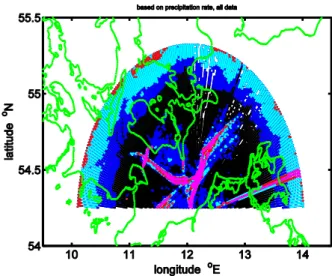
To minimize the effect of erroneous data caused, e.g., by moving ships or wind turbines, all grid points with mean rain rates exceeding plus-minus one standard deviation from the total mean, were excluded (Figure 2). These grid points also show much higher frequencies of precipitation (not shown). To take into account that rain rates are not Gaussian distributed, the bootstrap method was used to compute the standard deviations [30]. ERA-Interim grid points were simulated as a 0.75° × 0.75°
average over a three hour interval. Simulated collocated observations were taken from the same three hour interval within the 0.75° × 0.75° area. Observations are simulated by 2 × 2 radar pixels, which is an area of approximately 2 × 4 km2, to take into account that precipitation measurements took place on moving ships, covering a distance of about 5 km during an 8 min interval. In accordance with the typical numbers of collocated observations over the Baltic Sea (Section 3.1) we have randomly chosen 15 simulated observations for each ERA-Interim grid point.
Figure 2. Mean rain rates derived by applying Equation (1) to Rostock radar reflectivities of the volume scan of the lowest available level. The colors indicate data which lie out of the given interval:
blue: 0.0475 ± 0.5 × 0.0175 mm·h−1; cyan: 0.0475 ± 0.0175 mm·h−1; red: 0.0475 ± 1.5 × 0.0175 mm·h−1; magenta: 0.0475 ± 2 × 0.0175 mm·h−1, where 0.0475 mm·h−1 is the total mean and 0.0175 mm·h−1 is the estimated standard deviation of all available weather radar data.
Figure 2.Mean rain rates derived by applying Equation (1) to Rostock radar reflectivities of the volume scan of the lowest available level. The colors indicate data which lie out of the given interval: blue:
0.0475˘0.5ˆ0.0175 mm¨h´1; cyan: 0.0475˘0.0175 mm¨h´1; red: 0.0475˘1.5ˆ0.0175 mm¨h´1; magenta: 0.0475˘2ˆ0.0175 mm¨h´1, where 0.0475 mm¨h´1is the total mean and 0.0175 mm¨h´1is the estimated standard deviation of all available weather radar data.
4. Results
4.1. Binary Statistics
In general, results of binary statistics between point measurements and areally/temporally-averaged estimates are difficult to interpret. For example, the probability to detect a precipitation event by a point measurement is smaller than by an areally/temporally-averaged estimate. As a consequence, the bias score is expected to take values greater than 1. To get an idea of reasonable values, the contingency tables (Tables1and2) are derived from the collocated events, as well from simulations (Section3.3). Results for the POD, bias score, critical success ratio, success ration, and accuracy are given in Table3. For comparison, the results are given for simulated collocated data based on radar reflectivities. All numbers are quite similar so it can be stated that ERA-Interim precipitation, despite to systematic deviations in the rain rates, shows, in general, a good agreement with observations for the Baltic Sea area. A relatively high number of false alarms, mainly caused by the high precipitation frequency of the ERA-Interim data, is obvious and was also found in several studies (e.g., [11] or [12]), as mentioned in the introduction.
Table 1. Contingency table for binary statistics of collocated events of ERA-Interim rain data and rain measurements on ships. The total number of collocated events is 205,557. The numbers of the proportions to the total number are also given.
ERA: No Rain ERA: Rain
ship: no rain measured correct negatives 121,412 = 59.1% false alarms 43,485 = 21.2%
ship: rain measured misses 10,265 = 5.0% hits 30,395 = 14.8%
Table 2. Contingency table for binary statistics collocated events of simulated fields and simulated rain observations based on weather radar data. The total number of collocated events is 32,685.The numbers of the proportions to the total number are also given.
Simulated Fields: No Rain Simulated Fields: Rain simulated observations: no rain correct negatives 27,321 = 83.6% false alarms 3078 = 9.4%
simulated observations: rain misses 549 = 1.7% hits 1737 = 5.3%
Table 3. Probability of detection (POD), critical success index (csi), bias score, success ratio, and accuracy for collocated events of ERA-Interim rain data with rain measurements and simulated data according to contingency Tables1and2.
ERA and Measurements Simulated Data
POD 0.7475 0.7598
csi 0.3612 0.3238
bias score 1.8170 2.1063
success ratio 0.4114 0.3607
accuracy 0.7385 0.8890
4.2. Annual Precipitation
Mean annual fields are based on more than 200,000 collocated events, each containing 15 to 16 collocated observations (Section3.1). To make reliable estimates only grid points based on more than 10,000 pairs of collocated data are taken into account. The agreement between ship measurements and ERA-Interim precipitation is good (Figure3); mean values and standard deviations are 0.079˘0.025 mm¨h´1derived from ship measurements, and 0.075˘0.016 mm¨h´1derived from the ERA-Interim estimates. Differences between the fields are well within one standard deviation, estimated by the bootstrap method [30]. With respect to annual fields, please note that all situations with solid precipitation were excluded.
Atmosphere 2016, 7, 82 6 of 13
Table 3. Probability of detection (POD), critical success index (csi), bias score, success ratio, and accuracy for collocated events of ERA-Interim rain data with rain measurements and simulated data according to contingency Tables 1 and 2.
ERA and Measurements Simulated Data
POD 0.7475 0.7598
csi 0.3612 0.3238
bias score 1.8170 2.1063
success ratio 0.4114 0.3607
accuracy 0.7385 0.8890
4.2. Annual Precipitation
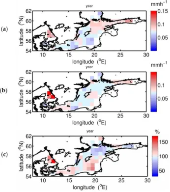
Mean annual fields are based on more than 200,000 collocated events, each containing 15 to 16 collocated observations (Section 3.1). To make reliable estimates only grid points based on more than 10,000 pairs of collocated data are taken into account. The agreement between ship measurements and ERA-Interim precipitation is good (Figure 3); mean values and standard deviations are 0.079 ± 0.025 mm·h−1 derived from ship measurements, and 0.075 ± 0.016 mm·h−1 derived from the ERA-Interim estimates. Differences between the fields are well within one standard deviation, estimated by the bootstrap method [30]. With respect to annual fields, please note that all situations with solid precipitation were excluded.
Figure 3. Mean annual precipitations rates in mm·h−1 derived from collocated precipitation events; (a) observations, (b) ERA-Interim, (c) ratio of ERA-Interim to observed precipitation rates.
4.3. Seasonal Precipitation
Seasonal comparisons give a different picture. In spring (MAM) ERA-Interim underestimates precipitation compared with measurements; in summer (JJA) the observed precipitation agrees nicely with the reanalyzed precipitation while, in autumn (SON), ERA-Interim overestimates precipitation (Figure 4).
(a)
(c) (b)
Figure 3.Mean annual precipitations rates in mm¨h´1derived from collocated precipitation events;
(a) observations, (b) ERA-Interim, (c) ratio of ERA-Interim to observed precipitation rates.
Atmosphere2016,7, 82 7 of 13
4.3. Seasonal Precipitation
Seasonal comparisons give a different picture. In spring (MAM) ERA-Interim underestimates precipitation compared with measurements; in summer (JJA) the observed precipitation agrees nicely with the reanalyzed precipitation while, in autumn (SON), ERA-Interim overestimates precipitation
(FigureAtmosphere 2016, 7, 82 4). 7 of 13
(a)
(b)
(c)
Figure 4. Seasonal estimates of stability and ratios of the ERA-Interim precipitation rate to measured precipitation rate derived from collocated events: (a): spring (MAM); (b): summer (JJA); and (c):
autumn (SON). Upper panels gives the frequencies of stable and unstable stratification (0%: none unstable stratification; 50%: in 50% of all cases stratification is unstable; 100%: always unstable stratification), bottom panels show precipitation ratios.
These biases might be correlated with atmospheric stability, which undergoes certain changes throughout the year, with prevailing stable conditions in spring and unstable conditions in autumn, Figure 4. Seasonal estimates of stability and ratios of the ERA-Interim precipitation rate to measured precipitation rate derived from collocated events: (a): spring (MAM); (b): summer (JJA);
and (c): autumn (SON). Upper panels gives the frequencies of stable and unstable stratification (0%: none unstable stratification; 50%: in 50% of all cases stratification is unstable; 100%: always unstable stratification), bottom panels show precipitation ratios.
These biases might be correlated with atmospheric stability, which undergoes certain changes throughout the year, with prevailing stable conditions in spring and unstable conditions in autumn, and is closely related to evaporation or latent heat flux. To check this assumption, stability in terms of Monin Obukov length has been estimated using a bulk flux scheme [23], in the following called the GEOMAR bulk flux scheme. Stability estimates are derived from ERA-Interim products. Figure4 shows the relative frequency of unstable and stable conditions, in comparison to the ratio of reanalyzed to measured precipitation. Indeed, ERA-Interim overestimates precipitation during prevailingly unstable conditions in autumn, and underestimates it during prevailingly stable conditions in spring, while during the summer months, where the occurrence of stable and unstable stratification is balanced, the agreement between measurements and reanalysis data is good. For the winter months no analysis is possible due to mostly snowy conditions.
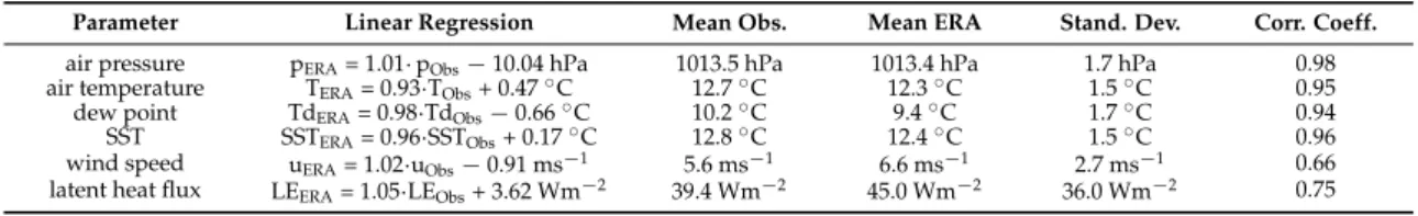
However, estimates of stability might be influenced by thus far unknown uncertainties in the reanalyzed input parameters for the bulk routines: temperatures, wind speed, humidity, and air pressure. To check this, independent ship observations have been used, reducing the observed air temperature, humidity, and wind speed stability-dependency from 18 m height [25] to 2 m and 10 m height, respectively, and comparing them to the ERA-Interim data (Table4). Except for wind speed, the agreement is good between the reanalysis products and observations; biases are generally small and correlation coefficients are 0.94 and more. Results also show that the difference of air and sea surface temperature is not biased. Therefore, the sign of stability is only somewhat affected due to the small differences in the regression coefficients. However, wind speeds are biased by about 1 m/s and show a large scatter, which is reflected in a low correlation coefficient of 0.65.
Table 4. Comparison of ERA-Interim (ERA) air pressure p, 2 m air temperature T, 2 m dew point temperature Td, SST, 10 m wind speed u, and latent heat flux LE derived from instantaneous evaporation to observations (Obs) from the SWA marine dataset, reduced to 2 m or 10 m height by applying the GEOMAR bulk flux scheme. The latent heat flux from observations was also computed by using the GEOMAR bulk flux scheme. The linear regression is derived from a forward and inverse linear regression weighted by the variances to take into account errors in both ERA-Interim and ship data.
Parameter Linear Regression Mean Obs. Mean ERA Stand. Dev. Corr. Coeff.
air pressure pERA= 1.01¨pObs´10.04 hPa 1013.5 hPa 1013.4 hPa 1.7 hPa 0.98
air temperature TERA= 0.93¨TObs+ 0.47˝C 12.7˝C 12.3˝C 1.5˝C 0.95
dew point TdERA= 0.98¨TdObs´0.66˝C 10.2˝C 9.4˝C 1.7˝C 0.94
SST SSTERA= 0.96¨SSTObs+ 0.17˝C 12.8˝C 12.4˝C 1.5˝C 0.96
wind speed uERA= 1.02¨uObs´0.91 ms´1 5.6 ms´1 6.6 ms´1 2.7 ms´1 0.66 latent heat flux LEERA= 1.05¨LEObs+ 3.62 Wm´2 39.4 Wm´2 45.0 Wm´2 36.0 Wm´2 0.75
This has consequences for the uncertainties of the related flux of latent heat. The positive bias in wind speed, in combination with slightly too dry air, leads to a small positive bias of 5.7 W/m2in ERA-Interim instantaneous evaporation expressed in terms of latent heat flux, compared to the latent heat flux based on ship observations using the GEOMAR bulk flux scheme. The correlation coefficient is 0.75 due to scatter in wind speeds. To check whether this is caused by the used bulk flux scheme, a comparison with the COARE algorithm [24] was performed. Results depict a pretty good agreement in terms of estimated latent heat fluxes between both bulk flux schemes. The correlation coefficient is 0.999 and the COARE bulk flux scheme gives only slightly higher fluxes, the bias to the GEOMAR bulk flux scheme is 2.7 W/m2.
4.4. Influence of Stability on Precipitation
Thus, it is possible to estimate the ratio of ERA-Interim precipitation to measured precipitation as a function of latent heat fluxes (Figure5). Latent heat fluxes were calculated by using the ERA-Interim temperature, humidity, wind speed, and pressure information as input values of the GEOMAR bulk flux scheme. The gray shaded area gives the ratio, plus/minus one standard deviation. It was
Atmosphere2016,7, 82 9 of 13
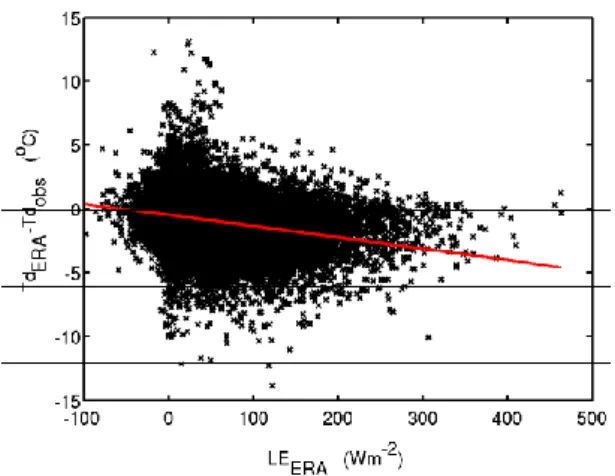
discovered that ERA-Interim gives too low precipitation values at low or slightly negative latent heat fluxes, though this result is not significant. With increasing latent heat flux, however, ERA-Interim increasingly overestimates precipitation up to a factor of two, which is significant for latent heat fluxes exceeding 130 Wm´2. This may indicate that the convection in the ERA-Interim reanalysis scheme is overestimated. As shown in a report of [32] there is a causal relationship between convection and temporal changes in humidity in the IFS (ECMWF Integrated Forecasting System). The negative bias in humidity, compared to marine observations, increases with increasing latent heat flux (Figure6), but it is only spuriously significant.
Atmosphere 2016, 7, 82 9 of 13
ERA-Interim reanalysis scheme is overestimated. As shown in a report of [32] there is a causal relationship between convection and temporal changes in humidity in the IFS (ECMWF Integrated Forecasting System). The negative bias in humidity, compared to marine observations, increases with increasing latent heat flux (Figure 6), but it is only spuriously significant.
Figure 5. Ratio of ERA-Interim to observed precipitation rates as a function of latent heat fluxes, derived from ERA-Interim air pressure, air temperature, humidity, SST, and wind speed by applying the GEOMAR bulk flux scheme. The shaded area gives the standard deviation.
Figure 6. Difference between the ERA-Interim and observed dew point temperature as a function of the latent heat flux, derived from ERA-Interim air pressure, air temperature, humidity, SST, and wind speed by applying the GEOMAR bulk flux scheme. The red line gives the result of a linear regression.
4.5. Fresh Water Budget P − E
Estimates of precipitation (P) and latent heat fluxes (or evaporation (E)) allow the computation of the fresh water budget of the atmosphere and ocean. The mean precipitation of all collocated events is 657 mm·a−1 based on ERA-Interim data. The mean evaporation derived from ERA-Interim instantaneous evaporation is 557 mm·a−1, resulting in a fresh water flux of P - E = 100 mm·a−1. Observations give a higher annual precipitation of 692 mm·a−1 and a lower evaporation of 488 mm·a−1, which results in a P - E of 204 mm·a−1. Please take into account that these estimates also exclude situations with solid precipitation. According to the results of Section 4.4 ERA-Interim underestimates precipitation in April/May and strongly overestimates it in September/October compared to observations, while ERA-Interim precipitation agrees well with observed precipitation in July/August (Table 5). As expected, the Baltic Sea freshens in spring and becomes saltier in autumn, which is less prominent for ERA-Interim data than for observations (Table 5).
Figure 5. Ratio of ERA-Interim to observed precipitation rates as a function of latent heat fluxes, derived from ERA-Interim air pressure, air temperature, humidity, SST, and wind speed by applying the GEOMAR bulk flux scheme. The shaded area gives the standard deviation.
Atmosphere 2016, 7, 82 9 of 13
ERA-Interim reanalysis scheme is overestimated. As shown in a report of [32] there is a causal relationship between convection and temporal changes in humidity in the IFS (ECMWF Integrated Forecasting System). The negative bias in humidity, compared to marine observations, increases with increasing latent heat flux (Figure 6), but it is only spuriously significant.
Figure 5. Ratio of ERA-Interim to observed precipitation rates as a function of latent heat fluxes, derived from ERA-Interim air pressure, air temperature, humidity, SST, and wind speed by applying the GEOMAR bulk flux scheme. The shaded area gives the standard deviation.
Figure 6. Difference between the ERA-Interim and observed dew point temperature as a function of the latent heat flux, derived from ERA-Interim air pressure, air temperature, humidity, SST, and wind speed by applying the GEOMAR bulk flux scheme. The red line gives the result of a linear regression.
4.5. Fresh Water Budget P − E
Estimates of precipitation (P) and latent heat fluxes (or evaporation (E)) allow the computation of the fresh water budget of the atmosphere and ocean. The mean precipitation of all collocated events is 657 mm·a−1 based on ERA-Interim data. The mean evaporation derived from ERA-Interim instantaneous evaporation is 557 mm·a−1, resulting in a fresh water flux of P - E = 100 mm·a−1. Observations give a higher annual precipitation of 692 mm·a−1 and a lower evaporation of 488 mm·a−1, which results in a P - E of 204 mm·a−1. Please take into account that these estimates also exclude situations with solid precipitation. According to the results of Section 4.4 ERA-Interim underestimates precipitation in April/May and strongly overestimates it in September/October compared to observations, while ERA-Interim precipitation agrees well with observed precipitation in July/August (Table 5). As expected, the Baltic Sea freshens in spring and becomes saltier in autumn, which is less prominent for ERA-Interim data than for observations (Table 5).
Figure 6.Difference between the ERA-Interim and observed dew point temperature as a function of the latent heat flux, derived from ERA-Interim air pressure, air temperature, humidity, SST, and wind speed by applying the GEOMAR bulk flux scheme. The red line gives the result of a linear regression.
4.5. Fresh Water Budget P´E
Estimates of precipitation (P) and latent heat fluxes (or evaporation (E)) allow the computation of the fresh water budget of the atmosphere and ocean. The mean precipitation of all collocated events is 657 mm¨a´1based on ERA-Interim data. The mean evaporation derived from ERA-Interim instantaneous evaporation is 557 mm¨a´1, resulting in a fresh water flux of P - E = 100 mm¨a´1. Observations give a higher annual precipitation of 692 mm¨a´1 and a lower evaporation of 488 mm¨a´1, which results in a P - E of 204 mm¨a´1. Please take into account that these estimates also exclude situations with solid precipitation. According to the results of Section4.4ERA-Interim
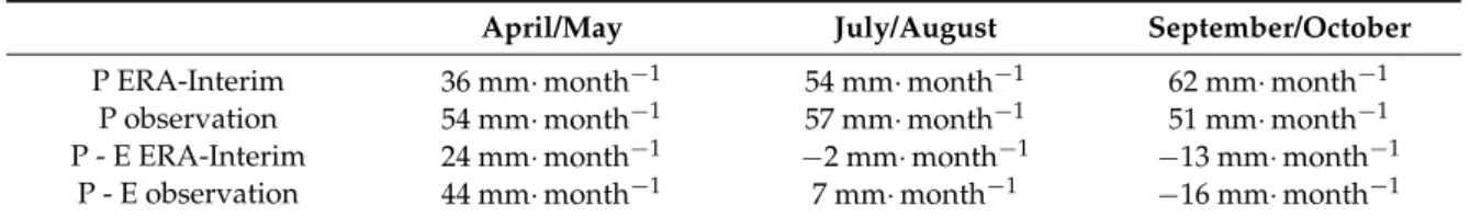
underestimates precipitation in April/May and strongly overestimates it in September/October compared to observations, while ERA-Interim precipitation agrees well with observed precipitation in July/August (Table5). As expected, the Baltic Sea freshens in spring and becomes saltier in autumn, which is less prominent for ERA-Interim data than for observations (Table5).
Table 5.Monthly precipitation P and fresh water budget P - E of ERA-Interim compared to collocated observations based on all collocated events.
April/May July/August September/October
P ERA-Interim 36 mm¨month´1 54 mm¨month´1 62 mm¨month´1
P observation 54 mm¨month´1 57 mm¨month´1 51 mm¨month´1
P - E ERA-Interim 24 mm¨month´1 ´2 mm¨month´1 ´13 mm¨month´1 P - E observation 44 mm¨month´1 7 mm¨month´1 ´16 mm¨month´1
5. Discussion
The main problem in interpreting the results is caused by the comparison of along-track point measurements with estimates integrated over time (ERA-Interim). Moreover, the strong spatial and temporal variability and intermittency of the precipitation further complicate the validation efforts.
Thus, we cannot expect a perfect agreement between the different datasets with respect to statistical parameters. To reduce this problem the data have been merged into events. To obtain an idea of reasonable statistical numbers, simulations of point-to-area collocations have been constructed based on weather radar reflectivities over the Baltic Sea. The summarized statistical parameters, compared to the results for simulations of point-to-area collocation, show a reasonable ability of ERA-Interim to detect precipitation. However, the results also show that ERA-Interim overestimates the frequency of precipitation, as has also been shown in earlier studies, see [11] or [12].
Nevertheless, averaged precipitation rates are close to the measured ones on an annual basis. However, a closer look on a seasonal basis reveals weaknesses related to stability and evaporation/latent heat fluxes. To ensure that this is not an artefact due to biases in ERA-Interim products, ERA-Interim atmospheric standard parameters,i.e., air temperature, sea surface temperature, dew point temperature, air pressure, wind speed, and evaporation (in terms of latent heat fluxes) have been validated against observations available in the SWA marine dataset. It was found that there are also considerable uncertainties in estimated latent heat fluxes mainly due to uncertainties in wind speed. These uncertainties are of the same order as given in a study of [33] for comparisons between measurements and different models over the Baltic Sea, biases in their study range from
´11.5 to 25 Wm´2, standard deviations from 29.5 to 46.8 Wm´2, and correlation coefficients from 0.61 to 0.78. In conjunction with a regression coefficient close to 1 (Table4), it can be concluded that the ERA-Interim products are of sufficient accuracy.
This allows relating the biases in ERA-Interim precipitation to latent heat fluxes. My main result is that there is a significant overestimation of ERA-Interim precipitation for situations with high evaporation. Following [34] or [22] this might be caused by uncertainties in the parameterization of the convection in the IFS. Consequently an overestimation of the precipitation indicates too much convection in the model, which should be related, according to [32], to atmospheric humidity. Indeed, it could be shown that ERA-Interim becomes drier with increasing latent heat fluxes compared to observations close to the surface. These data suggest investigating the convection scheme in detail, but this is not within the scope of this study.
Mean annual precipitation estimates should be taken with care, because data are restricted to rain data only. Nevertheless, estimated annual precipitation is only slightly higher than other estimates as [33] or [35], who gave values ranging from 600 to 640 mm¨a´1. This is to be expected because monthly precipitation during the winter season is lower than average monthly precipitation for the Baltic Sea area, see [33] or [35]. Estimated latent heat fluxes are comparable to other estimates, which are 39 to 44 Wm´2 [36] or 42 Wm´2 [35] The comparison of ERA-Interim latent heat fluxes with
Atmosphere2016,7, 82 11 of 13
estimates derived from observations shows that uncertainties in terms of bias and standard deviation are of the same order as found in other studies, see e.g., [33]. However it should be noted that even a typical bias in the latent heat flux of 5 W m´2gives a bias in annual evaporation of about 65 mm. With respect to the numbers given for P´E over the Baltic Sea such uncertainties are not negligible and call for a validation study of ERA-Interim evaporation over the Baltic Sea, as suggested by [1].
6. Conclusions
The comparison of the binary statistics based on the ERA-Interim product and collocated observations of rain, with results derived from simulated fields and observations based on weather radar reflectivities and the good agreement of the annual precipitation rates with observations, indicate that ERA-Interim precipitation is of sufficient accuracy over the Baltic Sea area. These fields can be used in combination, e.g., with ERA-Interim evaporation information, to estimate the annual fresh water budget, P - E.
However, the most important result is the overestimation of ERA-Interim precipitation with increasing evaporation. This has consequences for the sea surface salinity on a sub-annual time scale.
Using ERA-Interim data as input fields for ocean modelling, the ocean becomes too fresh for unstable atmospheric conditions in autumn, and less certain, too salty under stable atmospheric conditions, as are typical for spring. This correlation should also be investigated for areas over the open ocean, where the land influence, always present for a semi-enclosed sea like the Baltic Sea, can be neglected.
A number of precipitation measurements are also available for the Atlantic Ocean (e.g., [17] or [37]), which allow for such a study.
Acknowledgments:I would like to thank especially the masters and their crews, for supporting the precipitation measurements on board all merchant ships and research vessels. I would like to thank the Finnlines shipping agency for their cooperation, which made it possible to mount our instruments on their ships. Special thanks go to the German Weather Service, Seewetteramt, to make the marine data archive available, and the German Meteorological Service for the radar data. ERA-Interim data used in this study have been obtained from the ECMWF data server. My thanks go also to Lisa Neef for proofreading and to the unknown reviewers, which helped to improve the paper.
Conflicts of Interest:The author declares no conflict of interest.
Abbreviations
The following abbreviations are used in this manuscript:
ECMWF European Center of Medium Range Weather Forecast BALTEX The Baltic Sea Experiment
GPCP Global Precipitation Climatology Project
HOAPS Hamburg Ocean Atmosphere Parameters and Fluxes from Satellite Data IMERG Integrated Multi-satellitE Retrievals for Global precipitation measurement GPS Global Positioning System
IFS Integrated Forecasting System
SWA Seewetteramt Hamburg
DWD German Weather Service
Z Reflectivity
R Rain rate
POD Probability of detection csi Critical success index
p Air pressure
T Air temperature
Td Dew point temperature
SST Sea surface temperature
u Wind speed
LE Latent heat flux
P Precipitation
E Evaporation
References
1. Omstedt, A.; Elken, J.; Lehmann, A.; Leppäranta, M.; Meier, H.E.M.; Myrberg, K.; Rutgersson, A. Review progress in physical oceanography of the Baltic Sea during the 2003–2014 period.Prog. Oceanogr.2014,128, 139–171. [CrossRef]
2. Smedman, A.-S.; Gryning, S.-E.; Bumke, K.; Högström, U.; Rutgersson, A.; Andersson, T.; Batchvarova, E.
Precipitation and evaporation budgets over the Baltic Proper: Observations and modelling.J. Atmos. Ocean Sci.2005,10, 163–191. [CrossRef]
3. Trenberth, K.E.; Fasullo, J.T.; Mackaro, J. Atmospheric moisture transports from ocean to land and global energy flows in reanalyses.J. Clim.2011,24, 4907–4924. [CrossRef]
4. Dee, D.P.; Uppala, S.M.; Simmons, A.J.; Berrisford, P.; Poli, P.; Kobayashi, S.; Andrae, U.; Balmaseda, M.A.;
Balsamo, G.; Bauer, P.; et al. The ERA-Interim reanalysis: Configuration and performance of the data assimilation system.Q. J. R. Meteorol. Soc.2011,137, 553–597. [CrossRef]
5. Adler, R.F.; Huffman, G.J.; Chang, A.; Ferraro, R.; Xie, P.-P.; Janowiak, J.; Rudolf, B.; Schneider, U.; Curtis, S.;
Bolvin, D.;et al.The version-2 global precipitation climatology project (GPCP) monthly precipitation analysis (1979–Present).J. Hydrometeorol.2003,4, 1147–1167. [CrossRef]
6. Huffman, G.J.; Adler, R.F.; Arkin, P.; Chang, A.; Ferraro, R.; Gruber, A.; Janowiak, J.; McNab, A.; Rudolf, B.;
Schneider, U. The global precipitation climatology project (GPCP) combined precipitation dataset.Bull. Am.
Meteorol. Soc.1997,78, 5–20. [CrossRef]
7. Andersson, A.; Fennig, K.; Klepp, C.; Bakan, S.; Graßl, H.; Schulz, J. The Hamburg Ocean atmosphere parameters and fluxes from satellite data—HOAPS-3.Earth Syst. Sci. Data2010,2, 215–234. [CrossRef]
8. Andersson, A.; Klepp, C.; Fennig, K.; Bakan, S.; Graßl, H.; Schulz, J. Evaluation of HOAPS-3 ocean surface freshwater flux components.J. Appl. Meteorol. Climatol.2011,50, 379–398. [CrossRef]
9. Huffman, G.J.; Bolvin, D.T.; Nelkin, E.J. Integrated Multi-satellitE Retrievals for GPM (IMERG) Technical Documentation. Available online: http://pmm.nasa.gov/sites/default/files/document_files/IMERG_doc.
pdf (accessed on 26 April 2016).
10. Rhein, M.; Rintoul, S.R.; Aoki, S.; Campos, E.; Chambers, D.; Feely, R.A.; Gulev, S.; Johnson, G.C.; Josey, S.A.;
Kostianoy, A.;et al.Observations: Ocean. InClimate Change 2013: The Physical Science Basis; Stocker, T.F., Qin, D., Plattner, G.-K., Tignor, M., Allen, S.K., Boschung, J., Nauels, A., Xia, Y., Bex, V., Midgley, P.M., Eds.;
Cambridge University Press: Cambridge, UK; New York, NY, USA, 2013; pp. 659–740.
11. Belo-Pereira, M.; Dutra, E.; Viterbo, P. Evaluation of global precipitation data sets over the Iberian Peninsula.
J. Geophys. Res.2011,116. [CrossRef]
12. Thiemig, V.; Rojas, R.; Zambrano-Bigiarini, M.; Levizzani, V.; De Roo, A. Validation of satellite-based precipitation products over sparsely gauged African river basins. J. Hydrometeorol. 2012,13, 1760–1783.
[CrossRef]
13. Wang, J.J.; Adler, R.F.; Huffman, G.J.; Bolvin, D.F. An updated TRMM composite climatology of tropical rainfall and its validation.J. Clim.2014,27, 273–284. [CrossRef]
14. Hasse, L.; Großklaus, M.; Uhlig, K.; Timm, P. A ship rain gauge for use under high wind speeds.J. Atmos.
Ocean. Technol.1998,15, 380–386. [CrossRef]
15. Clemens, M. Machbarkeitsstudie zur Räumlichen Niederschlagsanalyse aus Schiffsmessungen Über der Ostsee. Ph.D. Thesis, Christian-Albrechts-Universität, Kiel, Germany, 2002.
16. Clemens, M.; Bumke, K. Precipitation fields over the Baltic Sea derived from ship rain gauge on merchant ships.Boreal Environ. Res.2002,7, 425–436.
17. Bumke, K.; König-Langlo, G.; Kinzel, J.; Schröder, M. HOAPS and ERA-Interim precipitation over sea:
Validation against shipboardin situmeasurements.Atmos. Meas. Tech.2016,9, 2409–2423. [CrossRef]
18. Froidurot, S.; Zin, I.; Hingray, B.; Gautheron, A. Sensitivity of precipitation phase over the Swiss Alps to different meteorological variables.J. Hydrometeorol.2014,15, 685–696. [CrossRef]
19. Kållberg, P. Forecast Drift in ERA-Interim ERA Report Series No 10. Available online: http://ecmwf.int/
publications/library/ecpublications/_pdf/era/era_report_series/RS_10.pdf (accessed on 11 April 2016).
20. Berrisford, P.; Kållberg, P.; Kobayashi, S.; Dee, D.; Uppala, S.; Simmons, A.J.; Poli, P.; Sato, H. Atmospheric conservation properties in ERA-Interim.Q. J. R. Meteorol. Soc.2011,137, 1381–1399. [CrossRef]
21. Over What Horizontal Area are Grid Point Data Values Valid? Available online: http://www.ecmwf.int/en/
faq/over-what-horizontal-area-are-grid-point-data-values-valid (accessed on 6 April 2016).
Atmosphere2016,7, 82 13 of 13
22. Sherwood, S.C.; Bony, S.; Dufresne, J.-L. Spread in model climate sensitivity traced to atmospheric convective mixing.Nature2014,505, 37–42. [CrossRef] [PubMed]
23. Bumke, K.; Schlundt, M.; Kalisch, J.; Macke, A.; Kleta, H. Measured and parameterized energy fluxes for Atlantic transects of R/V Polarstern.J. Phys. Oceanogr.2014,44, 482–491. [CrossRef]
24. Fairall, C.W.; Bradley, E.F.; Hare, J.E.; Grachev, A.A.; Edson, J.B. Bulk parameterization of air–sea fluxes:
Updates and verification for the COARE algorithm.J. Clim.2003,16, 571–591. [CrossRef]
25. Kent, E.C.; Woodruff, S.D.; Berry, D.I. Metadata from WMO publication No. 47 and an assessment of voluntary observing ship observation heights in ICOADS.J. Atmos. Ocean. Technol. 2007, 24, 214–234.
[CrossRef]
26. Rubel, F. Scale dependent statistical precipitation analysis. In Proceedings of the International Conference on Water Resources & Environment Research: Towards the 21st Century, Kyoto, Japan, 29–31 October 1996.
27. Kinzel, J.Validation of HOAPS Latent Heat Fluxes against Parameterizations Applied to RV Polarstern Data for 1995–1997; Christian-Albrechts-Universität Kiel: Kiel, Germany, 2013.
28. Obukhov, A.M. Turbulence in an atmosphere with a non-uniform temperature.Tr. Inst. Teor. Geofiz. Akad.
Nauk. SSSR1946,1, 95–115. [CrossRef]
29. Bartels, H.; Weigl, E.; Reich, T.; Lang, P.; Wagner, A.; Kohler, O.; Gerlach, N. in cooperation with the Meteo Solution GmbH RADOLAN, Routineverfahren zur Online-Aneichung der Radarniederschlagsdaten mit Hilfe von automatischen Bodenniederschlagsstationen (Ombrometer), DWD, Abteilung Hydrometeorologie, Zusammenfassender Abschlussbericht für die Projektlaufzeit von 1997 bis 2004. Available online: http://www.dwd.de/DE/leistungen/radolan/radolan_info/abschlussbericht_
pdf.pdf;jsessionid=FC016CC6C87FB0CF48708E2EADBB847F.live11041?__blob=publicationFile&v=2 (accessed on 13 April 2016).
30. Efron, B. Bootstrap Methods, another Look at the Jackknife.Ann. Stat.1979,7, 1–26. [CrossRef]
31. WWRP/WGNE. Methods for Dichotomous Forecasts. Available online: www.cawcr.gov.au/projects/
verification/#Methods_for_dichotomous_forecasts (accessed on 11 April 2016).
32. Bechtholt, P.Atmospheric Moist Convection; ECMWF: Reading, UK, 2015.
33. Hennemuth, B.; Rutgersson, A.; Bumke, K.; Clemens, M.; Omstedt, A.; Jacob, D.; Smedman, A.-S. Net precipitation over the Baltic Sea for one year using several methods.Tellus2003,55A, 352–367. [CrossRef]
34. Holloway, C.E.; Petch, J.C.; Beare, R.J.; Bechtold, P.; Craig, G.C.; Derbyshire, S.H.; Donner, L.J.; Field, P.R.;
Gray, S.L.; Marsham, J.H.;et al. Understanding and representing atmospheric convection across scales:
Recommendations from the meeting held at Dartington Hall, Devon, UK, 28–30 January 2013.Atmos. Sci.
Lett.2014,15, 348–353. [CrossRef]
35. Lindau, R. Energy and water balance of the Baltic Sea derived from merchant ship observations.
Boreal Environ. Res.2002,7, 417–424.
36. Döscher, R.; Meier, H.E.M. Simulated sea surface temperature and heat fluxes in different climates of the Baltic Sea.AMBIO2004,33, 242–248. [CrossRef] [PubMed]
37. Klepp, C. The Oceanic Shipboard Precipitation Measurement Network for Surface Validation—OceanRAIN.
Atmos. Res.2015,163, 74–90. [CrossRef]
© 2016 by the author; licensee MDPI, Basel, Switzerland. This article is an open access article distributed under the terms and conditions of the Creative Commons Attribution (CC-BY) license (http://creativecommons.org/licenses/by/4.0/).