Introducing the monotonicity constraint as an eﬀective chemistry-based condition in self-modeling curve resolution

(1)

Introducing the monotonicity constraint as an effective chemistry-based condition in self-modeling curve resolution

Somaye Vali Zade^a,b, Mathias Sawall^b, Klaus Neymeyr^b,c, Hamid Abdollahi^a

aFaculty of Chemistry, Institute for Advanced Studies in Basic Sciences, 45195-1159 Zanjan, Iran

bUniversität Rostock, Institut für Mathematik, Ulmenstrasse 69, 18057 Rostock, Germany

cLeibniz-Institut für Katalyse, Albert-Einstein-Strasse 29a, 18059 Rostock, Germany

Abstract

The results by soft modeling multivariate curve resolution methods often are not unique and are questionable because of the rotational ambiguity. It means a range of feasible solutions equally fits experimental data and fulfills the constraints. Regarding to chemometric literature, the reduction of the rotational ambiguity in multivariate curve resolution problems is a major challenge in order to construct effective chemometric methods. It is worth to study the effects of applying constraints on the reduction of the rotational ambiguity, since it can help us to choose the useful constraints for multivariate curve resolution methods for analyzing data sets. The aim of this work is to demonstrate the impact of monotonicity and unimodality constraints on the full set of all feasible, nonnegative solutions. We compared the results of two constraints in different two- and three-component systems. To reach this goal, two simulated kinetic and equilibrium data sets are used. Moreover, an experimental data set related to a mixture of two uniprotic acid solutions at different pH values as a model for equilibrium systems is used to extend the discussions to real cases. It is shown in this work that monotonicity is a meaningful chemistry-based constraint which in some cases is more effective than unimodality.

Keywords: Self-modeling curve resolution, Multivariate curve resolution, Rotational ambiguity, Monotone-unimodal areas, Unimodality constraint, Monotonicity constraint

1. Introduction

Multivariate curve resolution (MCR) is a powerful chemometric tool to investigate multivariate data sets, which has been widely used for resolving bilinear data sets obtained from the chemical processes in different application fields such as pharmaceutical analysis, agriculture, food chemistry, environment, and industrial and clinical chemistry [5]. MCR methods are divided into soft and hard approaches. Spectrophotometric data that describes a chemical process can be analyzed by using these two different approaches. Hard-modeling based methods require a chemical model to describe the process which is being investigated. Soft-modeling approaches, like multivariate curve resolution, are meant to describe processes without using explicitly the underlying chemical model linked to them [5].

By using soft modeling methods, we avoid the errors caused by choosing an incorrect model. At the same time, the signals originating from species that do not take part in the reaction are included in the analysis. However, the main drawback of these soft methods is the rotational ambiguity associated with the obtained profiles. In fact, there is an ambiguity to find the true decomposition. In order to decrease the ranges of feasible solution, the useful knowledge about the chemical system can be applied as constraint. Therefore, self-modeling curve resolution (SMCR) attempts to find all the feasible solutions regarding to certain restrictions. Several methods were reported to calculate all feasible solutions in two- and three-component systems.

The self-modeling curve resolution was first introduced by the pioneering work of Lawton and Sylvestre in 1971 [15]. Borgen and Kowalski [4] expanded this method for three-component systems on the basis of the non-negativity constraint, using the simplex rotation algorithm. However, the three-component system is more complex than the two-component problem and this algorithm was rather hard to comprehend and apply. Rajkó and István in 2005 utilized computational geometry tools in order to clarify the Borgen method, due to the complexity of using Borgen plots for three-component systems. They revised Borgen’s study and could elucidate the concepts of SMCR methods based on the geometry of the abstract space [20]. A systematic grid search for the calculation of all feasible solutions was proposed by Vosough et al. [30] for two-component systems. This was extended to three-component systems, and later on, for four-component systems by Golshan et al. [8]. These methods explore the set of feasible solutions that minimize the residual that is obtained from the difference between the real data set and the reconstructed data set.

Nevertheless, the concept of grid search methods is time consuming. Golshan et al. have developed an adaption of the simplex algorithm which reduces the number of computations [10]. Then Sawall et al. [22] have suggested a fast and

(2)

accurate algorithm to compute the Area Feasible Solution (AFS) in two- and three-component systems by using the polygon inflation algorithm. Recently, Jürß et al. [13] have introduced generalized Borgen plots for spectral data with small noise. Sawall et al. [21] have introduced the dual Borgen plots for the simultaneous computation of both AFS sets. And later on, they have introduced in a second part algorithmic enhancements that make the simultaneous Borgen plot construction possible for noisy experimental data matrices which can contain small negative matrix entries [23].

SMCR methods calculate all feasible solutions of the components in a system, while by construction the result of the MCR methods is always a single solution. Getting more information about a system and applying constraints in a suitable way will result in less ambiguity and under certain circumstances even unique answers can be achieved [16].

The useful constraints for restricting the rotational ambiguity are non-negativity, unimodality [6], hard modeling [9], local rank and selectivity [29, 28]. The first and most general natural constraint is non-negativity that is implemented on the concentration and response profiles [15]. Tauler et al. [28] studied intensity and rotational ambiguities as well as the effect of the selectivity and the local rank constraints on successful applications of MCR methods. They suggested that the presence and detection of the selectivity and appropriate use of constraints are the cornerstones of the individual MCR analyses. Unimodality is a common constraint that is applied to chromatographic elution profiles. It guarantees that chromatograms have just one maximum [6]. Beyramisoltan et al. suggest procedures for implementing equality and unimodality constraints in the Lawton-Sylvestre method and impose the equality on Borgen plots [2]. Hard modeling constraints on concentration profiles are powerful constraints which calculate profiles based on the chemical model and their mathematical function. These constraints resulted in unique solutions for components which can be described with a proper physical/chemical model [9]. On the other hand, applying some of the constraints such as local rank constraint can reduce the extent of rotational ambiguity. In some cases a unique solution can be achieved, Akbari et al. [1] have shown that this constraint is a mathematical concept that may not be in agreement with chemical information. Thus, applying local rank constraints in MCR methods can lead to incorrect solutions. In general, the constraints used for MCR and SMCR methods should be based on physical/chemical relevance. If they would only be based on mathematical concepts, they may not be in agreement with chemical information. Therefore, the constraints used for soft analysis should be based on reality. Among of the various constraints that have different effects to restrict the rotational ambiguity, the monotonicity constraint can be very helpful in some chemical systems because in these systems some species behave monotone. The concentration profiles of the reactants and products of a chemical reaction can usually be assumed as monotone decreasing or increasing functions. Thus, monotonicity constraints on these profiles can reduce the AFS. On the other hand, monotonicity is a restricted mode of unimodality. Therefore, in systems that components have a monotone behavior, if there are unimodal profiles (non- monotone profiles) in the set of feasible solutions are removed by the monotonicity constraint while these profiles are accepted by the unimodality constraint. So monotonicity constraints on these profiles can reduce the AFS more than the unimodality constraints. For first time, Sawall et al. [25] have demonstrated the impact of monotonicity constraint in soft constraints (monotonicity, unimodality and windowing) on the full set of feasible, non-negative solutions for a three-component system.

In this research work, we introduce the monotonicity constraint as a chemically meaningful restriction and empha- size the impact of monotonicity constraint in the study of kinetic and equilibrium chemical processes. Furthermore we investigated its efficiency compared to the unimodality constraint on the extent of rotational ambiguity in the simulated and spectroscopic data sets.

2. Theoretical basis

Second order bilinear data can be decomposed by multivariate curve resolution methods according to

D=CS^T+E (1)

In this equationD(k×n) is a spectral data matrix corresponding to a bilinear system withkdifferent samples andn different variables. The matrixC(k×s) includes the contributions of thescomponents in each sample,S (n×s) is the pure response matrix of the components andE(k×n) is the residual error matrix.

Given a spectral data matrixD, MCR methods try to obtain the two matricesC andS. For this purpose, the singular value decomposition or the principle component analysis (PCA) provide a decomposition of data matrix according to

D=UΣV^T =XV^T =UY^T (2)

According Eq. (2), the bilinear matrixDcan be decomposed toU that is the left singular vector matrix, V is the right singular vector matrix andΣis a diagonal matrix including the singular values. The matricesX andYinvolve coordinates of the projected row and column vectors of the matrixDin the row and column spaces, respectively. The problem of the SMCR technique is to acquire the correct basis profilesCandS for a given data set. The matricesX

(3)

andVcan be transformed by any invertible transformation matrixTto physically and chemically interpretable matrix, CandS based on

D=

XT⁻¹ T V^T

=

UT_∗⁻¹ T_∗Y^T

=CS^T. (3)

Note that the transformation matrices for the two spaces have one-to-one relationships: ΣT⁻¹ = T_∗⁻¹ andT =T∗Σ.

The matricesCandS may not be determined uniquely. Thus, in most cases, several transformation matricesT could generate matricesCandS that fit the data set equally well. Therefore, an infinite number of solutions are possible. All these feasible solutions are equally valid from a mathematical point of view, although only one of them is the true one.

This intrinsic indeterminacy of MCR methods is known as rotational ambiguity [15, 19]. In fact, the results of MCR methods are completed with two types of ambiguity, namely the intensity and rotational ambiguity. The intensity ambiguity can be removed by using a normalization for the single profiles. However, scaling cannot remove rotational ambiguity. Based on the rotational ambiguity, all feasible solutions have the same sum of squares residuals. So there is a range of feasible solutions forC andS^T related to the elements of the matrixT. However, when constraints are applied and the data structure is used appropriately, the set of feasible solutions can be reduced considerably.

This reduction can sometimes lead to a single unique solution. The most important constraint that can be applied is the non-negativity of the concentration values and the molar absorptivities as a natural property of most chemical systems. Additional constraints such as equality, hard-modeling, unimodality and monotonicity can also be applied and investigated by SMCR methods in order to reduce the rotational ambiguity.

2.1. Defining areas of feasible solutions for two- and three-component systems by the grid search method

To deal with rotational ambiguity problem, among the methods for the calculation of feasible solutions, the systematic grid search methods for two- and three-component systems [15, 4, 26] and also in the case of more complex multi-component mixture [7, 12, 14] are reformulated to find all feasible matrix T defining the correctC and S. Defining the sum of squared residuals (ssq) as a function of the matrix elements ofT is the heart of these methods. At the first step,CandS are estimated by the normalized transformation matrix according to (3). Normalization of the matrixT is useful (as mentioned) because it generally removes the intensity ambiguity and also reduces the unknown elements of the matrixT. In the next step, all the physical constraints are imposed on the profiles inCandS and the results in matricesC^∗andS^∗. Finally, the ssq is computed from the difference between the reconstructed data (C^∗and S^∗) and the original data set (D) according to

R=D−C^∗S^∗T, ssq=X

i

X

j

R²_{i j}.

In two-component systems (s=2) all decomposition matrices are formed by two columns or rows. In particular the transformation matrixT is a 2×2 matrix, and may be written as,

T = t11 t12

t21 t22

!

Since only the shapes of the concentration profiles and spectra are of interest and the scale may be fixed, it is legitimate to useT in the form

T = 1 t12

t₂₁ 1

!

(4) and the inverse ofT matrix is

T⁻¹= 1 1−t12t21

1 −t12

−t21 1

!

(5) ThenCandS^T are computed asC=UΣT⁻¹andS^T =T V^T. Thet12value defines the shape of the first spectrum and of the second concentration profile, apart from the normalization. Analogously, thet21value defines the shapes of the second spectrum and of the first concentration profile. A systematic grid search of all possible values oft12 andt21

exploring a comprehensive section of the space of feasible spectra and concentration profiles has been proposed. This approach allows the detection and visualization of the presence of rotational ambiguities in MCR solutions.

In case of three-component system, the matricesT have the dimensions 3×3. Accordingly, the ssq is a function of nine elements ofT matrix. In the grid search algorithm, the first column of the matrixT is fixed to 1 by dividing

(4)

each row of the matrixT by its first element. In this kind of normalization, the first coordinate of each profile on the first eigenvector will be 1 and feasible regions can be visualized in a 2D plane by dropping the first eigenvector.

T =







t11 t12 t13

t21 t22 t23

t31 t32 t33







→ T_normalized=







1 t12 t13

1 t22 t23

1 t32 t33







(6) The two elements of the matrixT related to one component feasible region are explored by a systematic search while the other four elements, which are other components coordinate, are calculated by a nonlinear optimization method (e.g by the standard simplex algorithm). A complete exploration of the coordinates of one component in the 2D space serves to find out the feasible region of that component. This process should also be repeated for the other two components in this space, and so it requires to apply grid search method 6 times to get the whole feasible regions for three components in two spaces.

2.2. Applying the unimodality constraints in SMCR methods

A unimodal concentration profile, typically the profile of an intermediate compound of a chemical reaction, has only one local maximum [27, 25]. Hence the function increases until the maximum is reached and decreases after- wards [27, 25]. Next A MatLab-code-element is presented for the computation of the unimodality constraint. This program code computes the cost value for a given factorC ∈R^(k×s). Therein the reference valueris either the last function value in the case of unimodal behavior or the last penalized decreased/increased value if the function is not in a unimodal way (thenY(j,i),0), see also [25]. A MatLab-code-element for implementing unimodality constraints reads as follows:

Y = zeros(k , s );

for i = 1: s

[r , i0 ] = max( C (: , i ));

for j = i0 : -1:2

Y ( j , i ) = min(0 , r - C (j -1 , i ));

if (( r > C (j -1 , i )) || (r - C (j -1 , i ) <0)) r = C (j -1 , i );

end end

r = C ( i0 , i );

for j = i0 +1: k

Y (j , i ) = min(0 , r - C (j , i ));

if (( r > C (j , i )) || (r - C (j , i ) <0)) r = C (j , i );

end end end

f_unimod = norm(Y , ' fro ')^2;

Finally the cost value on unimodality ofCis the squared Frobenius norm ofY(last line of the MatLab-code).

funimodal(C)=kYk²_F. (7)

2.3. Applying the monotonicity constraints in SMCR methods

This part of the paper contains a procedure how to implement the monotonicity constraints. The monotonicity constraints are applied to the concentration profiles. The heart of the monotonicity constraints is an objective function for detecting monotone profiles. The objective function is defined as

fmonotone(C)=X

min(kZ(:,i)k²₂,kW(:,i)k²₂), (8) see also [25]. Therein the variableZcontrols the monotone decreasing behavior and the variableWcontrols controls the monotone increasing behavior. For the computation ofZ andW the auxiliary variablesz,w ∈ R^(k×s) are used which are defined inductively. According to

z1,i=C1,i, w1,i=C1,i, i=1, ...s, (9)

The remaining entries ofzandware computed as z_j+1,i=











Cj+1,i, if zj,i>Cj+1,ior zj,i<Cj+1,i, zj,i otherwise,

(5)

wj+1,i=











Cj+1,i, if wj,i<Cj+1,ior wj,i>Cj+1,i,

wj,i otherwise, (10)

forj=1, ...,k−1. The matricesZandWare computed as

Zj,i=min(0,zj,i−Cj+1,i), Wj,i=max(0,wj,i−Cj+1,i),

fori = 1, . . . ,sand j = 1, ...,k−1. The objective function from (8) together with its auxiliary functions from (9) and (10) for applying the monotonicity constraints can be used in every multivariate curve resolution method. A MatLab-code-element for implementing the monotonicity constraints reads as follows:

Z = zeros(k , s );

W = zeros(k , s );

for i = 1: s z = C (1 , i );

w = C (1 , i );

for j = 1:length( C ) -1

Z (j , i ) = min(0 , z - C ( j +1 , i ));

W (j , i ) = max(0 , w - C ( j +1 , i ));

if (( z > C ( j +1 , i )) || (z - C ( j +1 , i ) <0)) z = C ( j +1 , i );

end

if (( w < C ( j +1 , i )) || (w - C ( j +1 , i ) >0 )) w = C ( j +1 , i );

end end end

f_mono (1 , i ) = min((norm( Z (: , i ) ,' fro ')) , (norm( W (: , i ) ,' fro ')))^2;

2.4. Outer polygon, inner polygon and the AFS

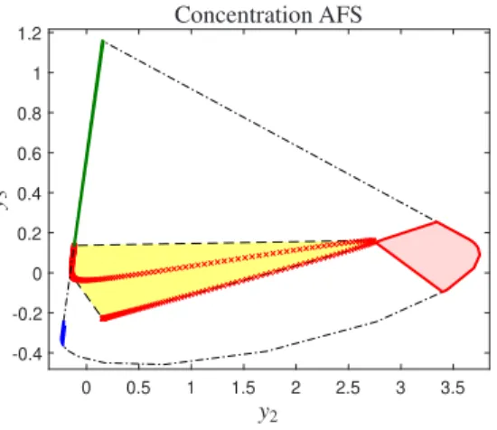
For a three-component system, the subspace of the pure components is three-dimensional. However, the geometry of the bilinear model in this system can be shown in 2D plane using some proper normalization. Fig. 1 displays the schematic illustration of the abstract space in three-component system (three-component equilibrium system, data set 2). This plot consists of three important sections: the outer polygon, the inner polygon and the AFS-sets [4, 20, 21].

The inner polygon is a convex polygon (convex hull) that encloses all the data points in the reduced abstract subspace (U- or V-subspace) after a proper normalization [18]. The convhull function as implemented in MatLabcan be used to identify the convex hull of the data points and so, the inner polygon. The sides of a polygon called outer polygon are the boundary between positive and negative sections of the abstract space. The transformed profiles from the facets (sides) of the outer polygon have at least one zero value and the hole inside this polygon will be the area where the transformed profiles have no negative values. For finding the vertices of the outer polygon is used to the duality concept [11, 17]. In [21, 23, 2] the duality has been used for the construction of the outer polygon and inner polygon for concentration and spectral spaces. Based on the concept of duality the vertices of the inner polygon in the V-space are dual to the facets of the outer polygon in the U-space. Moreover, the vertices of the inner polygon in the U-space are dual of the facets of the outer polygon in the V-space. In this term, the sides of any outer polygon can be calculated by using the dual vertices of the inner polygon. So, the inner polygon recognizes the convex hull of data points and the outer polygon as a non-negativity boundary, defines the border between positive and negative regions of abstract space [20, 17]. The AFS-sets contains all the possible solutions for the curve resolution problem and is placed between in the inner and the outer polygons. See Fig. 1 for the outer and the inner polygons as well as the AFS-sets for data set 2.

If the unimodality or monotonicity constraints are applied, then the set outer polygon in the U-space is restricted/reduced. This reduction has a direct effect to reduce the feasible regions in U-space, since some simplex- constructions (Borgen plots) are not possible any more. Due to the duality principle it has also an indirect reduction- effect in the V-space. How the outer polygon in U-space is reduced by the unimodality and monotonicity constraints is presented in Fig. 9 and Fig. 13.

3. Experimental section

The goal for simulated data is to investigate the effect of the monotonicity and unimodality constraints and to compare these two constraints on the range of feasible solutions. To reach this goal, we simulate kinetic and equilibrium data sets. The first simulated data set is a kinetic system consisting of two independent first-order reactions

(6)

0 0.5 1 1.5 2 2.5 3 3.5 -0.4

-0.2 0 0.2 0.4 0.6 0.8 1 1.2

y₂ y3

Concentration AFS

Figure 1: The AFS-sets (blue, green, red), the outer polygon (dash/dotted black line) and the inner polygon (dashed black line) for the simulated data set (data set 2). The red points indicate the columns of the data in concentration space.y2andy3are the second and third coordinates (scores) of the projected column vectors in the concentration space.

10 20 30 40 50

0.2 0.4 0.6 0.8

Time Concentration profiles

200 300 400

0.2 0.4 0.6 0.8

Wavelength Spectral profiles

200 300 400

0.1 0.2 0.3

Wavelength Mixed spectra

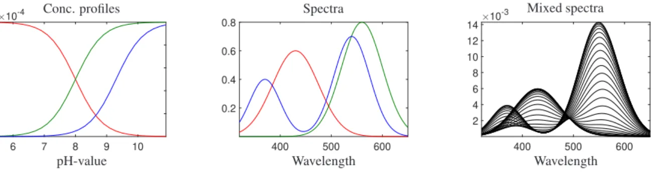
Figure 2: Data set 1: left panel shows the simulated concentration profiles; the central panel shows the simulated spectral profiles; the right panel shows the simulated absorbance data. Red: componentAblue: componentB.

for considering two-component system. The second simulated data set is an equilibrium system which consists of a mixture of two different uniprotic acid as a three-component system. Moreover, an experimental data set as a third data set was used to extend the discussions to real cases. The simulations were carried out in MatLaband the SMCR calculations for obtaining the Borgen plots and feasible solutions were made by the FACPACK software or the grid search method. Next the data sets are introduced in more detail.

3.1. Simulated kinetic systems

3.1.1. Data set 1: Two-component kinetic system

The first simulated data set is obtained from the concentrations and spectra in Fig. 2, corresponding to a mixture of two first order kinetic systems (A→^k¹ B,C→^k² D) monitoring with a spectrophotometer.

The speciesBand Dare spectroscopically active in the region under study. The data matrix contains mixture spectra at different times of reaction. The matrix hask =50 rows andn =281 columns. Spectral profiles for two species were created with Gaussian functions. The concentration profiles for these species were simulated according to the known model. When a matrix of two first-order kinetic reactions was modeled, the columns of the concentration matrix were calculated according to

[A]=[A0] e^−k¹^t, [B]=[A0]

1−e^−k¹^t , [C]=[C0] e^−k²^t, [D]=[C0]

1−e^−k²^t .

There are two monotone concentration profiles in this data matrix. The concentration profiles and the associated spectral feasible bands of each component are represented by same color.

3.1.2. Data set 2: simulated equilibrium system

The data set is created to model the spectrophotometric monitoring of a mixture of two uniprotic acid solutions at different pH-values. The data set consists of three species. The concentration profiles, the pure component spectra

(7)

6 7 8 9 10 2

4 6 8

10^-4

pH-value Conc. profiles

400 500 600

0.2 0.4 0.6 0.8

Wavelength Spectra

400 500 600

2 4 6 8 10 12 14 10^-3

Figure 3: Data set 2: The left panel shows the simulated concentration profiles; the central panel shows the simulated spectral profiles; the right panel shows the simulated absorbance data.

and the mixed spectra are shown in Fig. 3. Spectral profiles for three species are created with Gaussian functions. The concentration profiles for these species are simulated according to the known model. When a matrix of two uniprotic acids (HA and HB) is modeled, the columns of the concentration matrix are calculated according to

[HA]= CHAH⁺

([H⁺]+K_HA), A⁻= CHAKHA

([H⁺]+K_HA), [HB]= CHBH⁺

([H⁺]+KHB), B⁻= CHBKHB

([H⁺]+KHB).

The species HA, A and B are spectroscopically active in the region under study. This data set hask =28 rows by n=331 columns.

3.1.3. Data set 3: experimental data:

Phenol red and phenolphthalein are chemical compounds that are often used as indicator in acid-base titration.

Phenol red (PhR) is a weak acid with pKa=7.9. Its color exhibits a gradual transition from yellow (λmax=443nm) to red (λ_max=570nm) over the pH range 6.8 to 8.2. Above pH 8.2, phenol red turns a bright pink color.Phenolphthalein (Phph) belongs to class of dyes known as Pthalein dyes. It is a weak acid (pKa=9.4,λ_max=553nm), which is colorless in acidic conditions and magenta (bright pink) in an alkaline solution. Phenolphthalein is slightly soluble in water.

Phenolphthalein (Phph), phenol red (PhR) and other analytical reagents were obtained from Merck and were used without further purification. A stock solution of phenolphthalein (Phph) 10⁻³M were prepared by dissolving 0.016g in 10ml distilled water and also a stock solution of phenol red (PhR) 10⁻³M was prepared by dissolving 0.018g in 10ml distilled water. Mixtures of Phph and PhR 10⁻⁵M was prepared by dilution of stock solutions and diluted by Britton-Robinson buffer 0.1M to 10ml. Ten spectrophotometric signals of (Phph 10⁻⁵M) and (PhR 10⁻⁵M) mixtures were recorded in pH range 5.5−10.5. All of the solutions were prepared fresh. The pH-values of the solutions were adjusted by NaOH and then each solution was transferred into the cuvette and the spectrophotometric spectra were recorded. All spectrophotometry measurements were done on a Cary spectrophotometer (Varian, UV S-2100). The measurements were done using a 3 cm quartz cell. The pH measurements were carried out with a Metrohm 713 pH meter (Herisau, Switzerland) equipped with a combined glass electrode. The temperature was maintained at 25.0^◦C.

4. Results

This section reports on the results of an application of the monotonicity and unimodality constraints in the bilinear data matrices. Here, we investigate the influence of the monotonicity and unimodality constraints on reduction of rotational ambiguity in two- and three-component systems. The results are compared. The main question arises: is there any difference between the monotonicity and unimodality constraints for restricting the AFS-sets? Alternatively, is it possible for the monotonicity constraint to reduce the rotational ambiguity more than the unimodality constraint in some systems?

The objective functions from (7) and (8) for applying the unimodality and monotonicity constraints can be used in every multivariate curve resolution method. As mentioned in the previous sections, the reduction of the AFS by soft constraints is also analyzed in previous works but therein several soft constraints are used in combination, see also [3, 24] for the reduction of the AFS by the complementarity/duality theory. The ultimate goal of this work is to illustrate monotonicity as a meaningful, chemistry-based constraint which is for some kinetic and equilibrium systems more effective than the unimodality constraints for reducing rotational ambiguity. In order to investigate the accuracy of applying monotonicity constraints without any non-ideal behavior of real data, we initially used the simulated

(8)

-1.5 -1 -0.5 0 0.5 1 10^-25

10^-20 10^-15 10^-10 10^-5

t12resp.t21

ssq

Concentration space by nonnegativity

-1.5 -1 -0.5 0 0.5 1

10^-25 10^-20 10^-15 10^-10 10^-5

t12resp.t21

ssq

Concentration space plus unimodality

-1.5 -1 -0.5 0 0.5 1

10^-25 10^-20 10^-15 10^-10 10^-5

t12resp.t21

ssq

Concentration space plus monotonicity

-1.5 -1 -0.5 0 0.5 1

10^-25 10^-20 10^-15 10^-10 10^-5

t12resp.t21

ssq

Spectral space by nonnegativity

-1.5 -1 -0.5 0 0.5 1

10^-25 10^-20 10^-15 10^-10 10^-5

t12resp.t21

ssq

Spectral space plus unimodality

-1.5 -1 -0.5 0 0.5 1

10^-25 10^-20 10^-15 10^-10 10^-5

t12resp.t21

ssq

Spectral space plus monotonicity

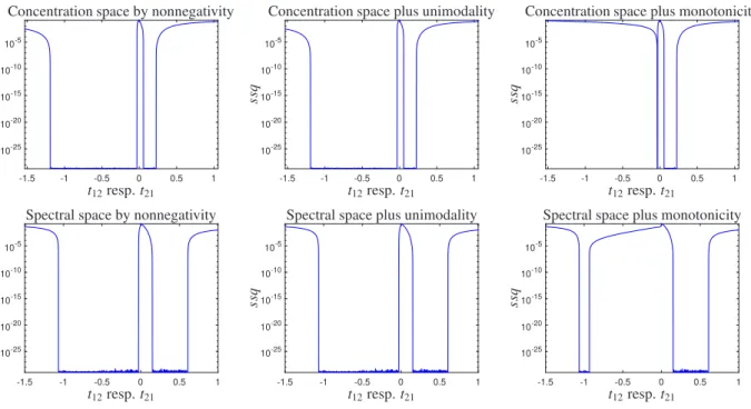
Figure 4: The concentrational and spectral feasible solutions for data set 1. First column: The feasible solution by using only the nonnegativity constraint. Second column: The feasible solutions by using the nonnegativity plus the unimodality constraint. Last column: The feasible solutions by using the nonnegativity plus the monotonicity constraint.

two- and three-component data sets. After that, an experimental data set is used to show the impact of applying monotonicity constraints in the real condition.

Fig. 2 (right panel) displays an appropriate noiseless two-component kinetic data set that is used for examination of the monotonicity and unimodality constraints. This data is obtained from multiplying simulated concentration profiles (left panel) by pure spectral profiles (center panel) in Fig. 2.

The SMCR results in the concentration and spectral subspaces acquired from the analysis of this system. The results are obtained by the grid search method when the nonnegativity, monotonicity and unimodality constraints are applied. In the first column of Fig. 4 we present semilogaritmic-plots of the sum of squares of the residuals as a function of thet- values (t12 resp. t21 from (4)) by using only the nonnegativity constraints for the simulated two- component kinetic system (data set 1). In the second and third columns of Fig. 4 we present semilogaritmic plots of the sum of squares of the residuals as a function of thet-values by using the nonnegativity plus the unimodality and monotonicity constraints for this system. The associated feasible profiles are plotted in Fig. 5. An important feature of the plots in Fig. 4 is the existence of a flat minimum region, respectively. Any set of coordinates in this minimum region results in different matricesCandS but the same productCS^T, and thus the solutions are not distinguishable;

they cover the range of all feasible solutions within rotational ambiguities. The whole range oft-values produces the whole feasible profiles of the first component spectrum (red) and of the second component concentration profile (blue).

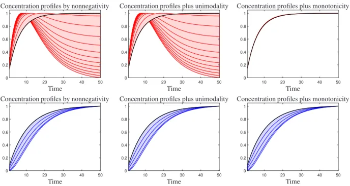
As shown in Fig. 5, there are non-monotone profiles (unimodal profiles) in the set of feasible profiles for the red component (the component related to the faster reaction). So the monotonicity constraint can reduce the AFS- sets and the set of feasible profiles related to one component concentration profile (red component) and reduce the AFS and the set of feasible profiles of the other component spectrum profile (blue component), There is a surprising cross-relationship. However, unimodality does not affect on reducing the AFS of this component because these non- monotone profiles are unimodal, as shown in the second and third columns of Figs. 5 and 6.

According to data based uniqueness rules, selectivity in concentration profiles or spectral profiles is very effective to reduce the amount of uncertainty of the solution, but it is generally not enough to obtain unique solutions in the other space. Therefore, the condition for a unique solution should be appropriate in both the concentration and the spectral space. Also in this data, as shown in Figs. 5 and 6, the nonnegativity constraint on its own is not enough to reduce the AFS and the range of feasible profiles. In contrast to this, By applying the monotonicity constraint the range of feasible solutions can considerably be reduced.

The effects of spectral overlapping on the impact of the unimodality and monotonicity constraints seem very dependent on the structure of the related data. In figuresS1 andS2 (see Supporting Information) the overlaid feasible bands of concentration profiles have been shown under two extreme spectral overlapping. In this case both constraints

(9)

10 20 30 40 50 0

0.2 0.4 0.6 0.8 1

Time

Concentration profiles by nonnegativity

10 20 30 40 50

0 0.2 0.4 0.6 0.8 1

Time

Concentration profiles plus unimodality

10 20 30 40 50

0 0.2 0.4 0.6 0.8 1

Time

Concentration profiles plus monotonicity

10 20 30 40 50

0 0.2 0.4 0.6 0.8 1

Time

10 20 30 40 50

0 0.2 0.4 0.6 0.8 1

Time

10 20 30 40 50

0 0.2 0.4 0.6 0.8 1

Time

Figure 5: Concentration feasible profiles being associated with the feasible solutions shown in the first column of Fig. 4. Nonnegative solutions (first column), unimodal nonnegative solutions (second column) and monotone nonnegative solutions (third column). Some representative profiles have been plotted in dark colors. The black lines represent the simulated concentration profiles

200 250 300 350 400 450

0 0.2 0.4 0.6 0.8 1

Wavelength

Spectral profiles by nonnegativity

200 250 300 350 400 450

0 0.2 0.4 0.6 0.8 1

Wavelength

Spectral profiles plus unimodality

200 250 300 350 400 450

0 0.2 0.4 0.6 0.8 1

Wavelength

Spectral profiles plus monotonicity

200 250 300 350 400 450

0 0.2 0.4 0.6 0.8 1

Wavelength

200 250 300 350 400 450

0 0.2 0.4 0.6 0.8 1

Wavelength

200 250 300 350 400 450

0 0.2 0.4 0.6 0.8 1

Wavelength

Figure 6: Spectral feasible profiles being associated with the feasible solutions shown in the second column of Fig. 4. Nonnegative solutions (first column), unimodal nonnegative solutions (second column) and monotone nonnegative solutions (third column). Some representative profiles have been plotted dark colors. The black lines represent the simulated spectral profiles

(10)

0 5 10 15 20 25 0

0.2 0.4 0.6 0.8 1 1.2

pH-value

0 5 10 15 20 25

0 0.2 0.4 0.6 0.8 1 1.2

pH-value

0 5 10 15 20 25

0 0.2 0.4 0.6 0.8 1 1.2

pH-value

0 50 100 150 200 250 300

0 0.05 0.1 0.15 0.2 0.25 0.3

Wavelength

0 50 100 150 200 250 300

0 0.05 0.1 0.15 0.2 0.25 0.3

Wavelength

0 50 100 150 200 250 300

0 0.05 0.1 0.15 0.2 0.25 0.3

Wavelength

Figure 7: Data set 2: The feasible profiles being associated with the AFS representations in Fig. 8. Nonnegative solutions (first column), unimodal nonnegative solutions (second column) and monotone nonnegative solutions (third column).

have been affected by the extent of spectral overlapping.

As well as, The effects of noise in the calculated area of feasible solutions have been investigated already in our group [8]. Generally, noise can increase the AFS of each profile due to improving the uncertainty of defined borders of feasible solutions regions. As monotonicity is a restricted mode of unimodality; therefore, that is expected to have the same effect of noise on both constraints.

The three-component equilibrium data set (data set 2) was analyzed by the systematic grid search method and the FACPACK software by using the non-negativity, unimodality and monotonicity constraints for concentrations and absorbances. Figure 8 shows the AFS-sets for all components in the concentration and spectral spaces for the data set 2. The color of each AFS-sets matches with the related component.

Every point in the feasible solution regions in U-space or V-space can be transformed to a concentration or spectral profile, respectively. Therefore, every feasible region can be transformed to a more interpretable concentration or spectral band profile. Figure 7 shows the feasible concentration and spectral profiles for all components in concentration and spectral spaces related to equilibrium system, the color of each AFS-sets matches with the color related component.

Three distinct feasible regions in Fig. 8 illustrate that rotational ambiguity exists for all three components. So, a range of feasible spectra can be defined for each species by the non-negativity constraints. The SMCR methods usually try to find a set of feasible spectra that can construct data with corresponding non-negative concentration profiles. Fig. 9 shows monotonicity/unimodality-areas for the outer polygon in the U-space for data set 2.

So, applying the monotonicity and unimodality constraints can decrease feasible region as shown in the second and the third columns of figure 8 for data set 2. The results show that the monotonicity constraints can reduce the AFS-sets in a harder way than unimodality (see the green component) . As shown in the Figs. 9 and 8, there are points in the AFS for the green component representing unimodal functions. Thus the monotonicity constraint can eliminate these points and reduces the AFS-subset of this component more than the unimodality constraints.

Nevertheless, if the monotonicity constraint is applied incorrectly and due to a wrong diagnosis to profiles which have a peak, in this case, it can lead to the removal of some acceptable responses. For instance, to consider a typical complexometric titration which chemical model is as follow

M+L↔ML K1=10^6.38 ML+L↔ML2 K2=10^11.91

WhereL(ligand), MLandML₂ are spectroscopic active species so the data set consists of three species. 10ml of ligand (8×10⁻⁶) titrated with 3ml metal ion (10⁻⁶). The concentration profiles were simulated in MatLabusing the Newton Raphson algorithm. Spectral profiles for three species are created with Gaussian functions. This data

(11)

0 1 2 3 0

0.5 1

y₂ y3

Concentration AFS by nonnegativity

0 1 2 3

0 0.5 1

y₂ y3

Concentration AFS plus unimodality

0 1 2 3

0 0.5 1

y₂ y3

Concentration AFS plus monotonicity

0 0.5 1 1.5 2 2.5 3

-0.4 -0.2 0 0.2 0.4

x2

x3

Spectral AFS by nonnegativity

0 0.5 1 1.5 2 2.5 3

-0.4 -0.2 0 0.2 0.4

x2

x3

Spectral AFS plus unimodality

0 0.5 1 1.5 2 2.5 3

-0.4 -0.2 0 0.2 0.4

x2

x3

Spectral AFS plus monotonicity

Figure 8: Data set 2: The concentrational and spectral AFS for a three-component equilibrium system. First column: The feasible solution by using only the nonnegativity constraint. Second column: The feasible solutions by using the nonnegativity plus the unimodality constraint. Last column:

The feasible solutions by using the nonnegativity plus the monotonicity constraint. (Dotted lines show the monotonicity areas.)

0 0.5 1 1.5 2 2.5 3 3.5

-0.4 -0.2 0 0.2 0.4 0.6 0.8 1 1.2

monotone unimod., not mono.

not unimodal

y₂ y3

Monotonicity/unimodality-areas for outer polygon (concentration)

Figure 9: Monotonicity and unimodality areas for outer polygon in concentration space for data set 2. Orange color is used to indicate monotone profiles, yellow color is used to indicate unimodal profiles which are not monotone and blue color indicates an area that is not related to unimodal or monotone profiles.

50 100 150

1 2 3 4 5 6

x 10⁻⁶

vadded

Concentration profiles

400 450 500 550 600

0.2 0.4 0.6 0.8 1 1.2 1.4 1.6

Wavelength Spectral profiles

400 450 500 550 600

2 4 6 8 10

x 10⁻⁶

Figure 10: Left panel shows the simulated concentration profiles; the central panel shows the simulated spectral profiles; the right panel shows the simulated absorbance data. Red: speciesLblue: speciesML2green: speciesML.

(12)

50 100 150 0.2

0.4 0.6 0.8 1

vadded

50 100 150

0.2 0.4 0.6 0.8 1

vadded

50 100 150

0.2 0.4 0.6 0.8 1

vadded

50 100 150

0.2 0.4 0.6 0.8 1

vadded

50 100 150

0.2 0.4 0.6 0.8 1

vadded

50 100 150

0.2 0.4 0.6 0.8 1

vadded

50 100 150

0.2 0.4 0.6 0.8 1

vadded

50 100 150

0.2 0.4 0.6 0.8 1

vadded

50 100 150

0.2 0.4 0.6 0.8 1

vadded

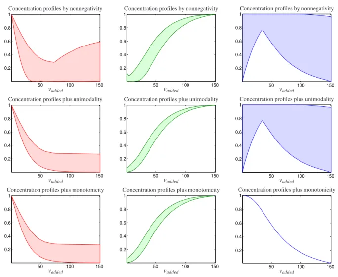
Figure 11: Concentration feasible profiles. The first row shows nonnegative solutions, the second row shows unimodal nonnegative solutions and the third row shows monotone nonnegative solutions. The first column is related to theL. The second column is related to theML. The third column is related to theML2.

set hask =151 rows byn =201 columns. The concentration profiles, the pure component spectra, and the mixed spectra are shown in Fig. 10. As shown in the figure, the concentration profiles ofLandMLare monotone and the concentration profile ofML2is unimodal. Next, the simulated data were analyzed and feasible solutions are obtained when the nonnegativity, monotonicity, and unimodality constraints are applied. Feasible profiles are plotted in Fig.

11. As it is clear from Fig. 11, applying monotonicity and unimodality constraints can decrease feasible profiles of LandMLspecies similarly. However, because exist monotone profiles in the set of feasible solutions for theML2

species (the unimodal species), the monotonicity constraint leads to the removal of some acceptable responses. Thus, after applying the monotonicity constraint incorrectly even unique answers can be achieved and removed acceptable responses.

Data set 3 is on the equilibrium system

1)Phenol red HA↔H+A pKa=7.9 2)Phenolphthalein HB↔H+B pKa=9.4

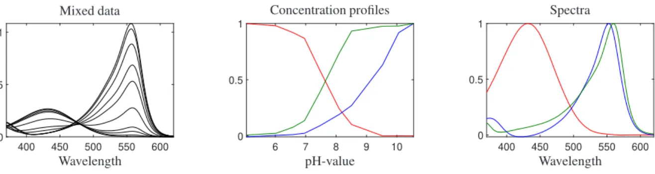
The experimental data set (10rows×251columns) consists of the spectra of the mixture samples (containing Phph and PhR) in different pH-values. The initial concentrations of PhR (HA) and Phph (HB) are 10⁻⁵M. This data, in spite of the simultaneous equilibrium, does not suffer from a rank deficiency. Phenolphthalein is colorless in acidic conditions and thus its protonated form (HB) does not show absorbance. Therefore, effectively we have a three- component system and there is not any rank deficiency. Fig. 12 represents the decomposition of the experimental data to the concentration and spectral profiles.

The AFS-sets are computed by using the FACPACK software under the non-negativity, unimodality and monotonicity constraints and the results are checked by using the systematic grid search method. The results coincide for each single restriction-level with respect to different control parameters. Data set 3 documents the monotonicity

(13)

400 450 500 550 600 0

0.5 1

Wavelength Mixed data

6 7 8 9 10

0 0.5 1

pH-value Concentration profiles

400 450 500 550 600 0

0.5 1

Wavelength Spectra

Figure 12: Data set 3: The left panel is related to the data set of the mixture samples of phph and phr in different pH; the center panel is related to concentration profiles and the right panel is related to spectral profiles.

0 1 2 3 4

-0.5 0 0.5 1

monotone unimod., not mono.

not unimodal

y2

y3

Monotonicity/unimodality-areas for outer polygon (concentration)

Figure 13: Monotonicity and unimodality areas for outer polygon in concentration space for the data set 3. Orange color is used to indicate monotone profiles, yellow color is used to indicate unimodal profiles and blue color indicates profiles that are not related to unimodal and monotone profiles.

constraints is not only helpful for simulated data sets but also for experimental, noisy data. Since species show a monotonous behavior. As it has been shown in Figs. 13, 14 the AFS-subsets of the green component contains points that are related to the orange area (monotone), the yellow area (unimodal but not monotone) and the blue area (not unimodal). The unimodality constraints removes the blue area and it accepts the orange and yellow areas. Consequently, the AFS of this component divided into two subsets, the monotone and unimodal subsets, while the monotonicity constraints just accepts the orange area, that means the subset which is related to the monotone profiles and removes two other areas. Therefore, this results show a similar behavior as explained above for the simulated model data, namely a drastic reduction of the AFS-sets by the monotonicity constraints.

The results are consistent with previous observations and the monotonicity constraint is more effective than the unimodality constraint for reducing the AFS-sets related to one species (green).

We have seen very clearly in Figs. 5 and 6 that the additional application of the monotonicity constraint compared to only applying the unimodality constraint can strongly reduce the rotational ambiguity. To a smaller extent, this result is confirmed by the experimental data set 3, see Fig. 14. Our analysis is closely related to the question of the reliability of MCR methods. We conclude that a soft-constraint MCR method can provide reliable results if this constraint of the MCR methods characteristically reduce the size of the AFS.

5. Conclusion

In this work the monotonicity and unimodality constraints are used for the reduction of the rotational ambiguity underlying multivariate curve resolution methods. In particular the reduction of the AFS-sets is investigated. The monotonicity constraint has already been studied in [25] for a three-component system. However, the difference of the monotonicity and unimodality constraints has not been mentioned clearly in the previous work. For the given data, our work obviously shows that the monotonicity constraint can reduce the AFS more than the unimodality constraint.

(14)

0 1 2 3 4 -0.5

0 0.5 1

y₂ y3

Concentration AFS by nonnegativity

0 1 2 3 4

-0.5 0 0.5 1

divided subset

y₂ y3

Concentration AFS plus unimodality

0 1 2 3 4

-0.5 0 0.5 1

y₂ y3

Concentration AFS plus monotonicity

0 1 2 3 4

-0.2 0 0.2 0.4 0.6

x2

x3

Spectral AFS by nonnegativity

0 1 2 3 4

-0.2 0 0.2 0.4 0.6

divided subset

x2

x3

Spectral AFS plus unimodality

0 1 2 3 4

-0.2 0 0.2 0.4 0.6

x2

x3

Spectral AFS plus monotonicity

Figure 14: Data set 3: The concentrational and spectral AFS for a three-component equilibrium system. First column: The feasible solution by using only the nonnegativity constraints. Second column: The feasible solutions by using the nonnegativity plus the unimodality constraints. Last column: The feasible solutions by using the nonnegativity plus the monotonicity constraints.

2 4 6 8 10

0 0.2 0.4 0.6 0.8 1

pH-value

2 4 6 8 10

0 0.2 0.4 0.6 0.8 1

pH-value

2 4 6 8 10

0 0.2 0.4 0.6 0.8 1

pH-value

Concentration profiles plud monotonicity

50 100 150 200 250

0.1 0.2 0.3 0.4 0.5 0.6 0.7 0.8 0.9

Wavelength Spectral profiles by nonnegativity

50 100 150 200 250

0 0.2 0.4 0.6 0.8 1

Wavelength Spectral profiles plus unimodality

50 100 150 200 250

0 0.2 0.4 0.6 0.8 1

Wavelength

Figure 15: The feasible profiles being associated with the experimantal data set. Nonnegative solutions (first column), unimodal nonnegative solutions (second column) and monotone nonnegative solutions (third column). The black lines show the original profiles.

(15)

So, monotonicity is a meaningful, chemistry-based constraint in these systems for reducing rotational ambiguity. Of course, if the monotonicity constraint is applied incorrectly and due to a wrong diagnosis to profiles which have a peak, in this case, it can lead to the removal of some acceptable responses.

The present study justifies the general recommendation to use any available information on the chemical reaction system in order to reduce ambiguity. The AFS approach enable a systematic access for the understanding and visualization of the implementation of such constraints.

References

[1] M. Akbari Lakeh, R. Rajkó and H. Abdollahi. Local rank deficiency caused problems in analyzing chemical data.Anal. Chem., 89(4):2259–

2266, 2017. PMID: 28192909.

[2] S. Beyramysoltan, H. Abdollahi and R. Rajkó. Newer developments on self-modeling curve resolution implementing equality and unimodality constraints.Anal. Chim. Acta, 827:1–14, 2014.

[3] S. Beyramysoltan, R. Rajkó and H. Abdollahi. Investigation of the equality constraint effect on the reduction of the rotational ambiguity in three-component system using a novel grid search method.Anal. Chim. Acta, 791:25–35, 2013.

[4] O. S. Borgen and B. R. Kowalski. An extension of the multivariate component-resolution method to three components. Anal. Chim. Acta, 174:1–26, 1985.

[5] A. de Juan, E. Casassas and R. Tauler.Soft modeling of analytical data. American Cancer Society, 2006.

[6] A. de Juan, Y. Vander Heyden, R. Tauler and D. L . Massart. Assessment of new constraints applied to the alternating least squares method.

Anal. Chim. Acta, 346(3):307–318, 1997.

[7] P. J. Gemperline. Computation of the range of feasible solutions in self-modeling curve resolution algorithms. Anal. Chem., 71(23):5398–

5404, 1999.

[8] A. Golshan, H. Abdollahi and M. Maeder. Resolution of rotational ambiguity for three-component systems. Anal. Chem., 83(3):836–841, 2011.

[9] A. Golshan, H. Abdollahi and M. Maeder. The reduction of rotational ambiguity in soft-modeling by introducing hard models.Anal. Chim.

Acta, 709:32–40, 2012.

[10] A. Golshan, M. Maeder and H. Abdollahi. Determination and visualization of rotational ambiguity in four-component systems.Anal. Chim.

Acta, 796:20–26, 2013.

[11] R. C. Henry. Duality in multivariate receptor models.Chemom. Intell. Lab. Syst., 77(1-2):59–63, 2005.

[12] R. C. Henry and B. M. Kim. Extension of self-modeling curve resolution to mixtures of more than three components: Part 1. Finding the basic feasible region.Chemom. Intell. Lab. Syst., 8(2):205–216, 1990.

[13] A. Jürß, M. Sawall and K. Neymeyr. On generalized Borgen plots. I: From convex to affine combinations and applications to spectral data.J.

Chemom., 29(7):420–433, 2015.

[14] B. M. Kim and R. C. Henry. Extension of self-modeling curve resolution to mixtures of more than three components: Part 2. Finding the complete solution.Chemom. Intell. Lab. Syst., 49(1):67–77, 1999.

[15] W. H. Lawton and E. A. Sylvestre. Self modelling curve resolution.Technometrics, 13(3):617–633, 1971.

[16] R. Manne. On the resolution problem in hyphenated chromatography.Chemom. Intell. Lab. Syst., 27(1):89–94, 1995.

[17] R. Rajkó. Natural duality in minimal constrained self modeling curve resolution.J. Chemom., 20(3-4):164–169, 2006.

[18] R. Rajkó. Studies on the adaptability of different Borgen norms applied in self-modeling curve resolution (SMCR) method. J. Chemom., 23(6):265–274, 2009.

[19] R. Rajkó. Additional knowledge for determining and interpreting feasible band boundaries in self-modeling/multivariate curve resolution of two-component systems.Anal. Chim. Acta, 661(2):129–132, 2010.

[20] R. Rajkó and K. István. Analytical solution for determining feasible regions of self-modeling curve resolution (SMCR) method based on computational geometry.J. Chemom., 19(8):448–463, 2005.

[21] M. Sawall, A. Jürß, H. Schröder and K. Neymeyr. Simultaneous construction of dual Borgen plots. I: The case of noise-free data.J. Chemom., 31(12):e2954, 2017.

[22] M. Sawall, C. Kubis, D. Selent, A. Börner and K. Neymeyr. A fast polygon inflation algorithm to compute the area of feasible solutions for three-component systems. I: Concepts and applications.J. Chemom., 27(5):106–116, 2013.

[23] M. Sawall, A. Moog, C. Kubis, H. Schröder, D. Selent, R. Franke, A. Brächer, A. Börner and K. Neymeyr. Simultaneous construction of dual Borgen plots. II: Algorithmic enhancement for applications to noisy spectral data.J. Chemom., 32(6):e3012, 2018.

[24] M. Sawall and K. Neymeyr. On the area of feasible solutions and its reduction by the complementarity theorem.Anal. Chim. Acta, 828:17–26, 2014.

[25] M. Sawall, N. Rahimdoust, C. Kubis, H. Schröder, D. Selent, D. Hess, H. Abdollahi, R. Franke, Börner A. and K. Neymeyr. Soft constraints for reducing the intrinsic rotational ambiguity of the area of feasible solutions.Chemom. Intell. Lab. Syst., 149:140–150, 2015.

[26] E. A. Sylvestre, W. H. Lawton and M. S. Maggio. Curve resolution using a postulated chemical reaction. Technometrics, 16(3):353–368, 1974.

[27] R. Tauler. Calculation of maximum and minimum band boundaries of feasible solutions for species profiles obtained by multivariate curve resolution.J. Chemom., 15(8):627–646, 2001.

[28] R. Tauler, A. Smilde and B. Kowalski. Selectivity, local rank, three-way data analysis and ambiguity in multivariate curve resolution. J.

Chemom., 9(1):31–58, 1995.

[29] R. Tauler, M. Viana, X. Querol, A. Alastuey, R.M. Flight, P.D. Wentzell and P.K. Hopke. Comparison of the results obtained by four receptor modelling methods in aerosol source apportionment studies.Atmos. Environ., 43(26):3989–3997, 2009.

[30] M. Vosough, C. Mason, R. Tauler, M. Jalali-Heravi and M. Maeder. On rotational ambiguity in model-free analyses of multivariate data.J.

Chemom., 20(6-7):302–310, 2006.