Prompt Gamma-ray 3D-Imaging for Cultural Heritage Purposes

Cultural Heritage Purposes

Inaugural-Dissertation zur Erlangung des Doktorgrades der Mathematisch-Naturwissenschaftlichen Fakultät

der Universität zu Köln

vorgelegt von

Ralf Schulze

aus Lemgo

Köln 2010

Prof. Dr. A. Eckart

Tag der mündlichen Prüfung: ^5.7.2010

wholesale returns of conjecture out of such a trifling investment of fact.

M ARK T WAIN

Die Entwicklung von neuen und die Verbesserung existerender element-sensitiver, bildgebender Verfahren mit Hilfe von Neutronen verschiedener Energiebereiche war das Ziel des europäischen A NCIENT C HARM -Projektes. Während der vorliegenden Arbeit wurde als Teil dieses Projektes die Station für Prompte-Gamma-Aktivierungs- Analyse (PGAA) am Forschungsreaktor FRM 2 in Garching bei München modifiziert, um die ortsauflösende Bestimmung elementare Verteilungen zu ermöglichen. Da sich die PGAA-Station am FRM 2 zu Beginn der Arbeit noch in der Fertigstellung befand wurden erste Tests und die Erarbeitung von ersten Kalibrierungs- und Messproze- duren für die neue bildgebende Methode von der Budapester PGAA-Gruppe in Ko- operation mit dem Institut für Kernphysik der Universität zu Köln am Budapester Forschungsreaktor vorgenommen. Auf Grund des höheren Neutronenflusses der Gar- chinger PGAA-Station wurden nach der regulären Inbetriebnahme der Station die benötigten Gerätschaften vom Budapester Reaktor zum FRM 2 verlegt. Dort wurden weitere Optimierungen vorgenommen und die Eigenschaften des Aufbaus charakte- risiert. Nach ersten Testmessungen mit Repliken von archäologischen Objekten wur- den mehrere Messungen an echten Objekten von ärchäologischem Interesse durchge- führt und analysiert. Hierbei wurden verschiedenen Messkonfigurationen angewen- det. Neben bildgebenden 2D- und 3D-Messungen wurde auch eine neue Anwendung zur Messung dünner Oberflächenschichten im Bereich von eingen 100 µ m entwickelt.

Für die quantitative Bestimmung von elementaren Verteilungen ist u. a. die ge- naue Kenntnis des Neutronenflusses an jeder gemessenen Position innerhalb der analysierten Probe nötig. Mit Hilfe der etablierten Methode der kalten Neutronen- Tomographie (NT) wurde ein Verfahren mit zugehöriger Software entwickelt, durch welches sich der erwartete Neutronenfluss innerhalb von Proben aus der mit NT ge- messenen Abschwächungs-Verteilung für kalte Neutronen bestimmen lässt.

Zur regulären Inbetriebnahme der PGAA-Station am Garchinger Forschungsreak- tor wurde u. a. ein neues Datenaufnahmesystem beigetragen, welches sowohl traditio- nelle PGAA-Messungen, als auch Messungen mit der neuen Methode der bildgeben- den PGA erlaubt. Durch die hohe Automatisierung erlaubt die neue Datenaufnahme einen deutlich effektiveren Betrieb der PGAA-Station, als es bisher der Fall war.

Die neue, momentan am Institut für Kernphysik der Universität zu Köln entwickel- te Software für die Analyse von _γ -Spektren „HDTV“ wurde um einige Funktionali- tät zur Analyse von PGAA-Spektren erweitert. „HDTV“ ist als zukünftiger moderner Nachfolger für die bisher genutzte Software „TV“ vorgeschlagen und erleichtert bspw.

die halb-automatische Analyse von vielen, ähnlichen _γ -Spektren, was für das neue

bildgebende PGA-Verfahren essenziell ist.

The development of new, and the enhancement of existing element-sensitive imaging methods utilizing neutrons of different energy regions was the aim of the European A NCIENT C HARM project. During the present work the setup for Prompt Gamma-ray Activation Analysis (PGAA) at the research reactor FRM 2 in Garching near Munich was modified to enable the spatial mapping of elemental abundances in the analysed samples. Because the PGAA setup at FRM 2 was under construction at the beginning of the project first tests and the development of calibration and measurement proce- dures for the new imaging method were done by the PGAA group at the Budapest Research Reactor in cooperation with the Institute for Nuclear Physics of the Uni- versity of Cologne. Due to the higher neutron flux at the PGAA setup at FRM 2 the equipment was transferred from the Budapest Research Reactor to FRM 2 after the PGAA setup at FRM 2 started its regular operation. After further optimizations and the characterization of the setup, measurements were started on replicas of real ar- chaeological objects before several measurements on real objects were performed and analysed. Several measurement configurations were applied. Additional to 2D and 3D imaging measurements a new application for the measurement of thin surface layers in the order of a few 100 µ m was developed.

For the quantitative analysis of elemental distributions the exact knowledge of the neutron flux at each measured position in the analysed sample has to be known.

Based on the well-established cold Neutron Tomography (NT) method a method and software have been developed, which enables the calculation of the neutron flux inside samples with the map of attenuation properties obtained through NT.

A new data acquisition system was developed for the regular operation of the PGAA setup at FRM 2, which supports traditional bulk PGAA measurements as well as measurements in the new imaging configuration. The high automation of the system allows a significantly more efficient use of the available measurement time than it was the case before.

The new software “HDTV” for the analysis of _γ -ray spectra, which is currently

under active development at the Institute for Nuclear Physics of the University of

Cologne, was extended by some functionality for the analysis of PGAA spectra. It is a

proposed modern successor of the currently used software “TV” and allows the semi-

automatic analysis of multiple, similar spectra, what is essential for the new imaging

PGA method.

1. Introduction 10

1.1. The use of neutrons for imaging purposes . . . . 10

1.2. The A NCIENT C HARM project . . . . 10

2. Neutron methods 13 2.1. Neutron properties . . . . 13

2.2. Neutron Tomography . . . . 14

2.2.1. Mathematical description . . . . 14

2.2.2. Cold Neutron Tomography . . . . 17

2.3. Prompt Gamma-ray Activation Analysis . . . . 18

2.3.1. Principle of the method . . . . 18

2.3.2. Quantitative PGAA . . . . 20

2.4. Prompt Gamma-ray Activation Imaging . . . . 21

2.4.1. Principle of the method . . . . 21

2.4.2. PGAI as a surface method . . . . 22

2.4.3. Quantitative PGAI . . . . 23

2.5. Combined PGAI and NT . . . . 24

3. Instrumentation 27 3.1. PGAA setup at FRM 2 . . . . 27

3.2. PGAI/NT setup at FRM 2 . . . . 27

3.2.1. Modifications to the PGAA setup . . . . 27

3.2.2. Alignment of the PGAI/NT setup . . . . 28

3.2.3. Design and properties of the _γ -collimator . . . . 32

3.2.4. Design and properties of the neutron collimator . . . . 35

3.3. Sample supports . . . . 40

3.4. Data acquisition system . . . . 43

3.4.1. Overview and requirements . . . . 43

3.4.2. Initial acquisition system . . . . 44

3.4.3. PGA-Acquisition-System (PAcSy) . . . . 45

4. Measurements and analyses 47 4.1. Sample positioning and registration . . . . 47

4.1.1. Introduction . . . . 47

4.1.2. Positioning . . . . 48

4.1.3. Registration . . . . 49

4.2. Calculation of the cold neutron flux inside samples . . . . 49

4.3. PGAI surface measurements on a bronze head . . . . 56

4.3.1. Object and motivation . . . . 56

4.3.2. Alignment of the setup and sample positioning . . . . 57

4.3.3. Analysis and results . . . . 59

4.4. Analysis of a proto-Corinthian vase . . . . 62

4.4.1. Object . . . . 62

4.4.2. Measurements . . . . 63

4.4.3. Results and discussion . . . . 63

4.5. Analysis of a bronze belt point from the 7 ^th century . . . . 65

4.6. Analysis of a 7 ^th century iron belt mount . . . . 66

4.6.1. Object . . . . 66

4.6.2. Measurements . . . . 67

4.6.3. Results . . . . 67

4.7. Analysis of a disc fibula from the 6 ^th century . . . . 67

4.7.1. Object . . . . 67

4.7.2. Measurements . . . . 69

4.7.3. Results . . . . 70

4.7.4. Discussion . . . . 73

5. Conclusions and outlook 83 A. Appendix 85 A.1. Nessas NT . . . . 85

A.2. PacSy hardware control libraries . . . . 87

A.2.1. Multi-Channel-Analyzer control . . . . 87

A.2.2. Sample table control . . . . 87

A.2.3. Beam control and safety management . . . . 89

A.2.4. Camera . . . . 91

A.3. FWHM approximation for the “bump” function . . . . 93

A.4. HDTV extensions . . . . 94

B. Acknowledgments 96

List of Figures 98

List of Tables 100

Bibliography 101

1.1. The use of neutrons for imaging purposes

The neutron is an ideal probe for the elemental and structural analysis of objects from multiple fields of interest, e.g. geology, crystallography, or archaeology. As chargeless particles the penetratoin depth of neutrons is large compared to e.g. X-rays or pro- tons and, depending on the used method, they can deliver the quantitative elemental composition of an investigated sample. Because neutrons interact with the nucleus, they can be used to identify different isotopes of one element.

Neutrons are in wide use for the bulk elemental, crystallographic or morphological analysis, but only few methods are established for position sensitive elemental dis- tribution measurements [Spy87, SK87, Bal96, Bae01, Kar03]. It was thus seen as desirable to form a collaboration for the joint development of new, non-destructive, element sensitive, 3D neutron imaging methods.

1.2. The Ancient Charm project

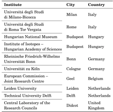
In 2006 the European A NCIENT C HARM ¹ project [Gor07] started as a collaboration of ten European Institutes (tab. 1.1) from the fields of physics and radiochemistry, ar- chaeology, restoration and conservation, and crystallography. The aim of A NCIENT

C HARM was the improvement of existing, and development of new neutron based 3D elemental imaging methods for the purpose of cultural heritage studies. The main methods used during the project were (cold) Neutron Tomography (NT), Prompt Gamma-ray Activation Analysis (PGAA) which has been developed into the imaging method Prompt Gamma-ray Activation Imaging (PGAI), Neutron Resonant Capture Analysis (NRCA) with the corresponding imaging method Neutron Resonant Capture Imaging (NRCI), and the newly developed Neutron Resonant (Transmission) Tomog- raphy (NRT).

Special focus was put on the combined analysis of the data-sets from the differ- ent methods with the aim of compensating the disadvantages of one methods with the results obtained through another method. E.g. NT is a method, which acquires highly resolved ( ≈ 100 − 500 µ m) 3D images in a relatively short time, but does not deliver elemental compositions. PGAI on the other hand has a much lower resolu- tion ( ≈ 3 − 6 mm) and requires much longer measurement times, but is able to deliver spatial elemental information. With the combination of these two methods (PGAI/NT), it is possible in some cases to obtain a quite accurate, high resolution elemental dis-

1

Analysis by Neutron resonant Capture Imaging and other Emerging Neutron Techniques: new

Table 1.1.: List of institutes that participated in the A NCIENT C HARM project

Institute City Country

Universitá degli Studi

Milan Italy di Milano-Bicocca

Universitá degli Studi

Rome Italy

di Roma Tor Vergata

Hungarian National Museum Budapest Hungary Institute of Isotopes –

Budapest Hungary Hungarian Academy of Sciences

Rheinische Friedrich-Wilhelms

Bonn Germany

Universität Bonn

Universität zu Köln Cologne Germany

European Commission –

Geel Belgium

Joint Research Centre

Leiden University Leiden Netherlands

Technical University Delft Delft Netherlands Central Laboratory of the

Didcot United

Research Councils Kingdom

tribution in acceptable measurement times without performing a full PGAI scan of the sample [Ebe09].

The tasks of the A NCIENT C HARM project were divided into several work-packages which covered (amongst others):

1. Selection of adequate samples for the final proof-of-concept measurements, 2. development of procedures for sample preparation and sample transport from

one measurement facility to another [Fes08],

3. fabrication of test and benchmark objects for the development and test of the different measurement methods [Kir08],

4. simulations for the design of new measurement setups and hardware [PC07, PC08, PC09a, PC09b],

5. development of PGAA into PGAI/NT and the construction of a new, high-flux PGAI/NT setup at the research reactor FRM 2 ² in Garching near Munich [Bel07, Kud08a],

2

Forschungs-Neutronenquelle Heinz Maier-Leibnitz, Technische Universität München:

http://www.frm2.tum.de/

6. development of NRCA into NRCI/NRT and the construction of a NRCI/NRT setup at the I SIS ³ pulsed neutron and muon source in Didcot, United Kingdom, 7. and the development of methods for the combination and mutual enhancement

of the data-sets obtained by the different methods [Sch09, Sch10].

The main involvement of the Institute of Nuclear Physics of the University of Cologne was in tasks 5 and 7 of the list above, but there was also participation in tasks 4 and 6.

3

I

Science and Technology Facilities Council, Rutherford Appleton Laboratory, Oxfordshire:

http://www.isis.stfc.ac.uk

2.1. Neutron properties

The free neutron is an unstable particle with a lifetime of 885.7(8) s. Its interesting feature for material analysis is that it is free of charge and can thus, unaffected of the atomic electron-shells, intrude deeply into materials. Neutron beams for material analysis are commonly created in nuclear research reactors or spallation sources.

The wavelength of a free neutron is given by the de Broglie equation:

λ = h

p = hc

p 2 E _kin m ₀ c (2.1)

For neutrons at “room temperature”, i.e. T = 293.16 K ⇒ E _kin = kT = 25.26 meV, one obtains the wavelength _λ = 0.1797 nm and the velocity v ₀ = 2198 m/s. Neutrons of this energy are called thermal neutrons. For further classification according to the neutron energies, and corresponding temperatures, the neutron energy spectrum is divided loosely into several groups [Mol04, Byr95]: Slow or cold neutrons with energies below about 100 meV, epithermal neutrons with energies in the range of about 0.1 eV – 1 eV, intermediate neutrons with about 1 eV – 1 MeV, and fast neutrons with energies above 1 MeV.

The important parameter for the description of neutron interaction with materials is the cross-section _{σ total} , which describes the overall probability of a nuclear reac- tion, i.e. scattering (elastic and inelastic) or capture, of a neutron with the irradiated nucleus:

σ total = σ scattering + σ capture . (2.2)

The cross-section of neutron capture reactions depends on the kinetic energy of the neutron. As a reference value for each isotope the neutron capture cross-section for thermal neutrons _{σ 0} is usually tabulated.

The energy dependence of neutron capture cross-sections shows a varying behavior in the different energy regions. Below thermal energy they follow the ¹ / v -law:

σ (v) : = σ capture (v) = v ₀

v · _{σ 0} , (2.3)

showing an inverse proportionality to the velocity. Going to higher neutron energies

the validity of this law is reduced, as resonances, i.e. energy regions where the cross-

section drastically increases in small energy windows, in the capture cross-section

value start to appear. Most resonances lie in the range of eV – keV, but some excep-

tional elements (Cd, Sm, Gd, and Eu) already show resonances in the thermal and

epithermal region [Mol04, Mug81, Mug84].

2.2. Neutron Tomography

2.2.1. Mathematical description

Tomography means the process of reconstructing the 2D-distribution of attenuation factors, elemental abundances or other sample properties ¹ from 1D-projections of these properties [Cor63, Hou73]. Performing this operation for a set of stacked slices one obtains a 3D-distribution of these properties from their 2D-projections, the so- called radiographies. These radiographies are taken during the rotation of the inves- tigated object ² around an axis perpendicular to the detection system. For a parallel illuminating beam theoretically a rotation for 180 ^◦ is enough, however in praxis it may be advisable to do a full 360 ^◦ rotation of the sample to compensate for deviations from the ideal theoretical assumptions ³ .

The principle of tomography is nicely explained in detail in e.g. [Kak88]. The fol- lowing summary is based on this reference.

Mathematically spoken the process of tomography is the determination of a 2D point function in one plane f (x, y) from its straight line integral values P _ϕ (t) [Rad17, Rad86]:

P _ϕ (t) = Z

line

f (x, y) ds. (2.4)

In praxis f (x, y) may be the distribution of neutron attenuation factors _µ (x, y) in one slice while P _ϕ (t) is a measure for the summed up attenuation factors along one line at angle _ϕ (fig. 2.1), i.e. the gray-value at “pixel” t in one slice of the radiography. Equa- tion (2.4) is called the Radon transform. With a parametrization in polar coordinates

t = x cos _ϕ + ysin _ϕ , (2.5)

we can rewrite (2.4) as P _ϕ (t) =

Z _+∞

−∞

Z _+∞

−∞ δ ¡

x cos _ϕ + ysin _ϕ − t ¢

f (x, y) dxdy. (2.6)

The key to the tomography problem is the Fourier-slice (or projection-slice) theo- rem [Bra56]. We take the 1D-Fourier transform of P _ϕ (t) and the 2D-Fourier trans- form of f (x, y):

P ϕ ( _ω ) = Z _+∞

−∞

P _ϕ (t) · e ^−2πiωt dt, (2.7)

F (u, v) = Z _+∞

−∞

Z _+∞

−∞

f (x, y) · e ^{− 2 π i (ux + v y)} dxdy. (2.8)

1

E.g. medical Computer Tomography (CT) maps X-ray attenuation factors in the human body, while medical Magnetic Resonance Imaging/Tomography (MRI/T) usually maps the distribution of hydro- gen.

2

In medical imaging it is common practice to rotate the detection system, not the “sample”, i.e. the screened patient. This is equivalent to the rotation of the sample.

3

E.g. in Neutron Tomography the effect of beam hardening, which describes the change of the neutrons

energy distribution on their way through the sample, influences the reconstruction results.

Figure 2.1.: The Fourier-slice theorem [Kak88, Pan83]

Looking at the special case v = 0 we obtain from (2.8) F (u, 0) =

Z _+∞

−∞

Z _+∞

−∞

f (x, y) d y

| {z }

P

(x)

· e ^{−2 π i (ux)} dx, (2.9)

and thus, using (2.7) and (2.9)

F (u, 0) = P ϕ= 0 (u) . (2.10)

Equation (2.10) is valid for all angles _ϕ , because for a rotated (t, s)-coordinate system

P ϕ (u) = F (u, v) (2.11)

is valid along a line which is rotated by _ϕ with respect to the u-axis (fig. 2.1). Express- ing eq. (2.6) in the (t, s)-coordinate system yields

P _ϕ (t) = Z _+∞

−∞

f (t, s) ds, (2.12)

(2.7)

⇒ P ϕ ( _ω ) = Z _+∞

−∞

Z _+∞

−∞

f (t, s) ds · e ^{−2 π i ω t} dt. (2.13) For reconstruction purposes it is desired to transform (2.13) to Cartesian coordinates:

P ϕ ( ω ) = Z _+∞

−∞

Z _+∞

−∞

f (x, y) · e ^{− 2 π i ω} ( ^xcos ϕ+ ysin ϕ ) dxd y. (2.14)

Figure 2.2.: Data point collection in the frequency domain by projections [Kak88, Pan83]

Inversion of the Fourier transform and using (2.11) with (u, v) = ( _ω cos _ϕ , _ω sin _ϕ ) gives:

f (x, y) = Z _+∞

−∞

Z _+∞

−∞ F (u, v) · e ^{− 2 π i (ux + v y)} du dv. (2.15) The Fourier-slice theorem can be summarized in words as:

The 1D-Fourier transform P _ϕ ( _ω ) of a parallel projection P _ϕ (t) at angle ϕ yields one slice, which subtends an angle _ϕ with the u-axis, in the 2D- Fourier transform F (u, v) of the projected distribution f (x, y) [Kak88].

With an infinite number of projections at different angles one could fill up the fre- quency domain by Fourier transformations of P ϕ (t) and then determine F (u, v). The searched distribution f (x, y) is then obtained via (2.15).

In reality the number of projections is not infinite and thus the number of known values of F (u, v) is limited. Because the projections are taken along radial lines, their density increases near to the center of the (u, v)-coordinate system (fig. 2.2). The re- construction is transferred to a Cartesian (x, y)-grid and due to the varying density of the data-points in the frequency domain they contribute differently to the Carte- sian reconstruction cells. Hence the data-points in the frequency domain have to be weighted by their distance to the coordinate origin.

Transforming the right side of (2.15) to polar coordinates ( _ω , _ϕ ) and under exploita- tion of the symmetry F ¡

ω , _ϕ + π ¢

= F ¡

− ω , _ϕ ¢ yields f (x, y) =

Z _π

0

Z _+∞

−∞ F ¡ ω , _ϕ ¢

| ω | · e ^{−2 π i ω} ( ^{x cos} ϕ+ysin ϕ ) d ω

| {z }

Q

( xcos ϕ+ysin ϕ )

d _ϕ . (2.16)

Figure 2.3.: A common Neutron Tomography setup

The term Q _ϕ is called filtered projection with filter | ω | . For practical reasons like e.g. noise filtering it may be advisable to use adjusted filters (e.g. the Shepp-Logan filter [Kak88]). Equation (2.16) is the basis for the filtered back-projection algorithm that is commonly used for tomographic reconstructions. Another alternative approach, based on the algebraic analysis of the projections, is introduced in [Bal07]. It is claimed that this algebraic reconstruction procedure performs better for cases when the projection information is incomplete, e.g. only available for a limited angular region.

During this work the software O CTOPUS [Die04], which uses the filtered back- projection algorithm, was used for the tomographic reconstructions.

2.2.2. Cold Neutron Tomography

For cold Neutron Tomography (NT) the reconstructed property is the distribution of neutron attenuation factors inside the investigated object. Modern NT systems, as shown in figure 2.3, acquire the radiographies with CCD ⁴ -cameras, that collect the image information digitally. The sample is placed on a rotation table into the cold neu- tron beam. A neutron scintillator, made e.g. from a ZnS:Ag, phosphor, and ⁶ Li com-

4

Charge-coupled device

pound, is placed behind the sample. This scintillator performs the reaction [Die04]

n + ⁶ Li → ³ H + ⁴ He + 4.79 MeV. (2.17) The ³ H and ⁴ He atoms interact with the phosphor in the scintillation layer and create visible light, which is collected by a grayscale CCD-camera. To protect the camera from neutron damages it is positioned outside the neutron beam, normally under an angle of 90 ^◦ . A silver-free ⁵ mirror reflects the light into the camera direction.

The theoretical number of projections of the sample one should acquire to obtain an optimal resolution is limited by the Nyquist theorem and results to:

# p = ^π N

2 , (2.18)

with the number of projections #p and the number of pixels in one horizontal slice of the detection system N. In [Sch99] it is shown that for realistic resolutions of the commonly used detector systems this number can be further reduced to

# p ≈ N

2 . . . 3 , (2.19)

without worsening the resulting reconstruction quality.

2.3. Prompt Gamma-ray Activation Analysis

2.3.1. Principle of the method

Prompt Gamma-ray Activation Analysis (PGAA) utilizes characteristic _γ -radiation that is emitted after the interaction of a nucleus with low energetic (thermal or cold) neutrons for non-destructive elemental or even isotopic identification and quantifica- tion measurements. It is closely related to Neutron Activation Analysis (NAA). PGAA is extensively described in the existing literature, e.g. [Mol04, Alf95, Pau00], thus only a brief summary is given here.

The most important process for PGAA and NAA is the radiative ¡ n, _γ ¢

-capture pro- cess. After the capture of a low energetic neutron (with an energy of a few meV) an excited compound nucleus is formed with an excitation energy of the neutron binding energy plus the kinetic energy of the neutron:

n + ^A Z → ^{A + 1} Z ^∗ . (2.20)

The neutron’s binding energy is the clearly dominating contribution, having values between about 6 MeV and 11.6 MeV for the known stable isotopes [Mol04]. The ex- cited nucleus then decays with the emission of _γ -radiation to its stable ground state, either directly or via energy levels between the excited and the ground state:

A+1 Z ^∗ → ^A+1 Z + γ . (2.21)

5

The irradiation of silver with neutrons induces long living activation, which should be avoided.

The intervals between the energy levels in the compound nucleus define the energies of the emitted _γ -rays, corrected for the recoil energy of the nucleus:

E _γ = E _Transition − E _Recoil , (2.22)

E _Recoil = E ² _γ

2 m _A c ² , (2.23)

with the mass of the recoiling atom m _A . For light elements the recoil energies can be in the order of up to some keV, thus about 3 magnitudes lower than usual transition energies.

The time scale of the decay processes defines the classification of prompt, i.e. “im- mediate” _γ -rays. One sensible definition for “promptness” can be given as:

Gamma-rays are called prompt, when their decay times, following the neutron capture reaction, are much shorter than the time resolution of the acquisition system [Mol04].

Typical time resolutions are in the order of nano-seconds, which defines the upper limit for the classification as prompt _γ -ray. The definition above clearly separates PGAA from NAA, where one looks at delayed _γ -rays following the neutron capture process, emitted by the formed daughter nucleus, usually after a _β ⁻ -decay. While for NAA the _γ -ray spectra acquisition is done offline, i.e. after the irradiation of the analyzed sample, PGAA acquisition has to be done online, i.e. during the irradia- tion of the sample by the neutron beam. Of course this leads to a much higher _γ -ray background in the PGAA spectra, which worsens the detection efficiency for many ele- ments compared to NAA. Taking into account that for PGAA the _γ -detector is usually placed farther away from the sample to avoid neutron damages, while for NAA the sample may be placed directly in front of the detector after sample activation (when the decay times of the investigated elements are long enough), the detection efficiency may be higher by a factor 50 or more for NAA [Sze08a]. Of course this is dependent on the investigated elements.

On the other hand PGAA is superior over NAA e.g. for some important light el- ements as H, B, N, Si, P, S, and Cl and some heavy elements as Cd, Gd, Sm and Hg [Yon96, Bae03, Fre08] which are difficult, or even impossible, to detect with NAA.

It thus can be seen as a complementary method to NAA. Another advantage of PGAA over NAA is the faster availability of the measurement results and the usually shorter irradiation times necessary.

For imaging purposes (see chapter 2.4), where multiple measurements have to be

performed on the same object at different positions and/or under different measure-

ment angles, the focus of PGAA on “immediately” decayed energy levels has the indis-

pensable advantage that subsequent measurements are not influenced by previous

irradiations, at least as long as the prompt gamma-ray peaks do not interfere with

longer living decay peaks.

2.3.2. Quantitative PGAA

PGAA is a quantitative method, i.e. it can deliver concentrations of elements in the investigated samples. However it is very difficult to obtain absolute values for the elemental masses inside a sample, due to factors like e.g. variations in the neutron flux over time, thus normally only a relative quantification is done. The elemental abundances are given relative to an internal standard element, that is present in the analyzed sample. One possible method for the quantification of elmental abun- dances is the k ₀ -method [Mol98, Pau95, Bae03, Lin03], which is originally coming from NAA [Sim75, Cor89].

The area of a peak at energy E _γ origination from the (n, _γ )-reactions on element _χ inside a sample volume V is given by [Mol98]:

N γ , χ ¡ E _γ ¢

= N _A Θ χ I _{γ , χ} M _χ ·

Z

V

Z _∞

E

= 0

Z _τ

t = 0 ρ _χ (V ) _{σ χ} (E _n ) Φ (E _n , t, V ) _² ¡ E _γ , V ¢

dt dE _n dV , (2.24) with the density _{ρ χ} (V ) = ^dm _dV

^{(V )} of the elemental mass dm _χ in volume dV , the Avo- gadro number N _A , the isotopic abundance Θ χ of the element’s isotope that emits the selected _γ -rays, the relative intensity of the investigated _γ -line I _γ , the atomic mass of the element M _χ , the (n, _γ )-cross-section _{σ χ} , the neutron flux distribution _φ at the selected volume, the overall detection efficiency _² of a _γ -ray emitted in the selected volume and the acquisition time _τ . For small, homogeneous samples and constant shape of the neutron flux distribution we can write [Gen00]:

Z

V ² ¡ E _γ , V ¢

dV = ² ¡ E _γ ¢

· f (V) , (2.25)

Z

v ρ _χ (V ) dV = m _χ , (2.26)

φ (E _n , t, V ) = ϕ (E _n , V ) · g (t) . (2.27) For the cold neutron region eq. (2.3) can be applied and we obtain for the peak ratios of element _χ to the internal monitor element _µ :

N _γ , χ ¡ E _{γ , χ} ¢ N γ , µ ¡

E _{γ , µ} ¢ = m _χ Θ _χ I _{γ , χ ²} ¡ E _{γ , χ} ¢

σ 0, χ ± M _χ m _µ Θ µ I _{γ , µ ²} ¡

E _{γ , µ} ¢ σ 0, µ ±

M _µ . (2.28)

The k ₀ -ratio of the elements _χ and _µ is then defined as:

k _{0,( χ , µ )} = N _γ , χ ¡ E _{γ , χ} ¢±

m _{χ ²} ¡ E _{γ , χ} ¢ N γ , µ ¡

E _{γ , µ} ¢±

m _{µ ²} ¡

E _{γ , µ} ¢ = Θ _χ I _{γ , χ σ 0, χ} ± M _χ Θ µ I _{γ , µ σ 0, µ} ±

M _µ . (2.29)

For the mass ratios of elements _χ and _µ one finally obtains:

m _χ m _µ = 1

k _{0,( χ , µ )} · N _γ , χ ¡ E _{γ , χ} ¢±

² ¡ E _{γ , χ} ¢ N γ , µ ¡

E _{γ , µ} ¢±

² ¡

E _{γ , µ} ¢ . (2.30)

The k ₀ -values for all isotopes are usually tabulated normalized to selected comparator

isotopes, e.g. hydrogen [IAE07].

2.4. Prompt Gamma-ray Activation Imaging

2.4.1. Principle of the method

Conventional PGAA is a bulk method, i.e. it delivers no information about the spa- tial distribution of the elements inside the sample. One direct method to obtain the spatial elemental distribution is Prompt Gamma-ray Activation Imaging (PGAI).

Through collimation or focussing of the neutron beam to a diameter of just few mil- limeter one limits the active measurement region to a small chord through the sam- ple [Bae01]. This is called the PGAI chord configuration (fig. 2.4(a)). The sample is then placed on a moving table that is able to position it in (at least) two dimensions in front of the collimated neutron beam, thus allowing a two dimensional scan of the whole sample or only some positions of interest. The analysis of the spectra obtained at the different positions then delivers a 2D elemental map of the investigated object.

(a) chord configuration (b) isovolume configuration

Figure 2.4.: PGAI measurement configurations (after [Kis08])

For three-dimensional elemental mapping the above procedure can be further ex- tended by a _γ -ray detector collimation of a few square millimeter [Kas06a, Kas06b, Kis08]. The intersection of the neutron beam with the solid angle of the collimated γ -ray detector then defines the spatially fixed, active measurement volume, the so- called isovolume (fig. 2.4(b)). Again scanning of the sample is performed, but through the _γ -collimation one now obtains the depth information about the elemental composi- tion along the neutron beam, which leads to a 3D elemental map of the object. Clearly, a table which supports movements in at least (x, y, z)-directions is needed as sample support, now. Anyhow it is advisable to use a sample support that allows rotation of the sample with respect to the beam, to be able to optimize the beam path through the sample, e.g. to minimize self-shielding effects.

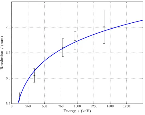
The physical dimensions of the isovolume limit the maximal achievable spatial res-

olution for the elemental mapping, hence it is desirable to make this volume as small

as possible. Of course the size of the isovolume directly influences the number of nu- clear ¡

n, _γ ¢

-reactions that can be detected and consequently the size of the isovolume should be chosen large enough to generate a “sufficient” number of _γ -events per time- interval in the detector, to keep the necessary measurement time acceptably short.

The choice of the isovolume dimensions is a compromise and has to be selected with regard to other parameters, like available neutron flux, detector efficiency, magnitude of _γ -ray background, and the cross-sections of the expected elements of interest.

2.4.2. PGAI as a surface method

The idea of PGAI as surface method is to use the 2D-PGAI chord-configuration with a thin chord neutron beam and open _γ -detector and to illuminate only a thin layer on the surface of the sample. With the help of neutron radiographies it is possible to align the sample in such a way that only a few hundred micrometer of the surface are illuminated (fig. 2.5). Care must be taken that only the desired sample position of the surface is illuminated by the neutron beam, because the unintended irradiation of other positions would give wrong additions to the collected spectra.

sample surface neutron beam

active measurement volume

Figure 2.5.: Principle of surface PGAI measurements

The advantage of using neutrons for the investigation of a small surface layer is again the bigger penetration depth of neutrons compared to e.g. protons. With an accurate sample-positioning it is possible to investigate thin layers of a few hundred micrometer, which is much deeper than what can be reached with e.g. PIXE, which can only be used for depths of some tens of micrometer [Kud05a]. For adequate geome- tries it is even possible to create a qualitative depth profile of the elemental densities at the sample surface. This can be interesting for the investigation of e.g. gilding layers on cultural heritage objects.

One problem of PGAI as surface method is that it requires a free line-of-sight along the analyzed surface, which is not given for all geometries, e.g. it is not possible to investigate positions in small valleys or channels on the sample. Another drawback is the time-consuming sample positioning (see chapter 4.3) and the need for a neutron radiograph.

Very first experiments with this PGAI configuration were conducted for this work

and are described in chapter 4.3.

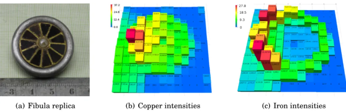
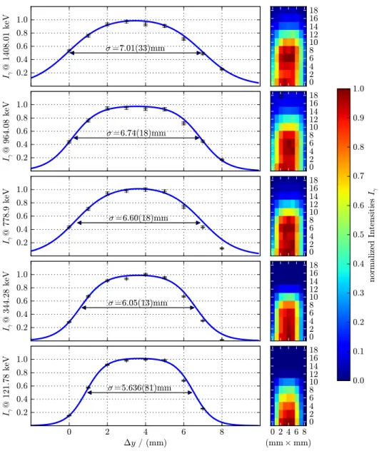
(a) Fibula replica (b) Copper intensities (c) Iron intensities

Figure 2.6.: Uncorrected elemental concentrations for copper and iron measured with a 2D- PGAI scan of the fibula replica (a). The γ -detector was positioned on the left side of the replica. ((b) and (c) courtesy of the Department of Nuclear Research, Institute of Isotopes, Hungarian Academy of Sciences, Budapest)

2.4.3. Quantitative PGAI

For the quantitative determination of elemental ratios with PGAI equation (2.24) that describes the peak areas generated from a small sample volume is valid in prin- ciple, but in contrast to the considerations in chapter 2.3.2 the k ₀ -method cannot be applied without corrections. Equation (2.30) was deduced for small, homogeneous samples. Obviously the approximation of a “homogeneous” sample makes no sense for an imaging method.

The problematic parameters for an elemental quantification are the neutron flux Φ _χ (E _n , V) at the isovolume position and the overall _γ -ray detection efficiency _² ¡

E _γ , V ¢ . In principle the distribution of the neutron flux Φ can be determined quite pre- cisely by measuring the flux quantity at isovolume position, e.g. via gold activation measurements, and applying the known neutron flux distributions Φ (E _n ) for the ap- propriate neutron production process [Mol04]. If we assume that the neutron flux does not fluctuate too much over time one then has a value for Φ (E _n , V _iso. ) without sample in the neutron beam. Unfortunately the sample material itself will disturb the neutron flux distribution (neutron self-shielding). This disturbance is dependent on the spatial distribution of the elements inside the sample and their concentrations, and thus exactly on the properties one wants to obtain.

Similar considerations are true for _² ¡

E _γ , V _iso. ¢

. For the determination of the overall

efficiency one has to respect the amount of _γ -rays that are absorbed on their way from

the isovolume to the detector ( _γ -ray self-absorption). This figure is dependent on E _γ

and again the elemental concentrations on the path from isovolume to sample surface

and can have a not negligible effect. This effect has been investigated with 2D-PGAI

measurements on the replica of an ancient fibula [Sze08b, Bel08c]. In figure 2.6 the

uncorrected copper and iron intensities that were measured over a grid covering the

whole object are shown. One clearly sees that the intensities on the side far away

from the detector are significantly smaller, than on the closer side, although, due to

the known manufacturing process, they are expected to be of the same magnitude.

The mentioned factors hamper the quantitative analysis of PGAI data significantly.

In chapter 4.2 an idea will be presented how to correct for the neutron self-shielding effect with the help of a NT reconstruction. For _γ -ray self-absorption correction it has been suggested to apply some Monte-Carlo simulations recursively to the measured PGAI data to reconstruct the elemental concentrations in multiple iterations [Sze08b].

For elements which emit _γ -rays over a wide energy range one may make use of the energy dependency of the absorption process to create a calibration function for self- attenuation correction [Pau95].

To sum up it has to be said that the problems for a true quantitative PGAI analysis are still unsolved, although some promising progress has been made (chapter 4.2).

2.5. Combined PGAI and NT

As indicated above, the high collimation of the neutron beam and, in case of isovol- ume measurements, the collimation of the _γ -detector cause a much lower event-rate for PGAI measurements compared to standard PGAA and thus much longer measure- ment times. For a full mapping of the object the needed measurement time per posi- tion has to be multiplied by the number of positions necessary for a full scan, hence significantly increasing the needed experiment time. E.g. to perform a full scan of a small cube of (10 × 10 × 10) mm ³ with an ideal isovolume size of (2 × 2 × 2) mm ³ one has to measure (5 × 5 × 5 = 125) positions. If we assume a necessary acquisition time of about 45 min per position the overall measurement time would be almost 4 days for this small object. For larger objects the required measurement time may become unrealistically long, e.g. for a cube of 20 mm edge lengths one would have to measure about one month for a full map with the above mentioned properties. Such a long measurement time is in most cases infeasible for several reasons:

• Experiment time at a PGAA/PGAI setup is often rare and valuable.

• The sample may not be available for very long measurements, e.g. objects of cultural heritage interest may be part of a permanent exhibition, where they can only be removed for relatively short times.

• Long irradiation times may cause activation of the sample. Depending on the activated isotopes the sample then has to stay at the measurement facility for a, possibly very long, decay period.

Although high, long-lasting activation of the sample is not so likely for PGAI mea- surements as it is for bulk PGAA, because always only a relatively small part of the sample is irradiated by neutrons, it still is the most severe argument for keeping the measurement times as short as necessary.

For many objects of interest it may be sufficient to measure just a few positions of

interest instead of performing a full PGAI scan, e.g. objects of cultural heritage in-

terest are often manufactured from many different parts, but each part for itself can

often be assumed to be of nearly homogeneous composition. For the selection of these

Figure 2.7.: Combined PGAI/NT setup

interesting positions the NT method may be utilized [Kas06b]. Because PGAI and NT both use a beam with low energetic neutrons these two methods may be operated at the same neutron beam guide in combination: NT for the initial acquisition of a 3D morphological model of the sample and the selection of interesting measurement posi- tions, and PGAI for the determination of the elemental composition at this positions.

NT can even assist in the final positioning of the sample for PGAI. This combined utilization of these two methods is called PGAI/NT [Bel08a, Bel08b, Sze08b].

In [Ebe09] a method is shown that utilizes NT to extend the elemental distribu-

tion, measured through a 2D-chord-PGAI for few distinct positions, to the complete

object. The idea is that adjacent regions that show the same neutron absorption prop-

erties in the NT reconstruction are probably made from the same material. E.g. it

is likely that a filling material that can be located in the NT reconstruction is quite

homogeneous all over the filled cavity, when it shows homogeneous neutron absorp-

tion properties. Of course this method is not completely accurate. Inhomogeneities

that are not visible via NT will falsify the elemental distribution. Another reason for

possible mistakes in the elemental 3D assignment may be the use of the chord geom-

etry. Because one always measures along a full line through the object, some parts

of the objects, e.g. a back-plate, may always be visible in the _γ -ray spectra and thus

lead to wrong assumptions. This effect may be minimized by a cleverly chosen set of

measurement positions and illumination angles of the sample in some cases, but not

in general.

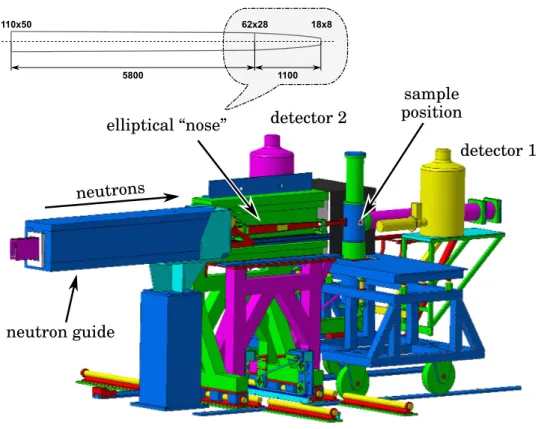
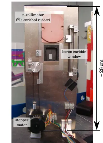
The design of a combined PGAI/NT setup is shown in figure 2.7. The sample is placed on a table that is movable in (x, y, z, _ω )-directions. For PGAI measurements a HPGe ⁶ - _γ -detector is placed at an angle of 90 ^◦ relative to the neutron beam. A _γ - collimator, normally made out of lead, is narrowing the detector’s field-of-view and defining the location of the isovolume in depth. Under the chosen angular orienta- tion the number of scattered neutrons that hit and damage the detector is minimized.

Another reason for this detector position is that in this way a regular, non-distorted isovolume can be defined together with the collimated neutron beam. A neutron colli- mator, e.g. fabricated out of ⁶ Li-enriched polymer, confines the neutron beam to a few millimeter diameter. For NT measurements the neutron collimator is removed to get a wide, open beam. The tomograph is located behind the sample table and should be positioned as close as possible to the sample, to minimize blurring effects.

6

High-Purity-Germanium

3.1. PGAA setup at FRM 2

The experiments were performed at the new PGAA setup at the Forschungsneutro- nenquelle Heinz Maier-Leibnitz (FRM 2) in Garching near Munich [Kud08a, Kud05b, Kud05a]. The setup is located at the end of a 51 m long cold neutron guide that is aiming at the cold source of the FRM 2 reactor core. A remarkable feature of the PGAA neutron guide is that its last 5.8 m are elliptically tapered, to focus the neutron beam and increase the available cold neutron flux. The guide can be extended by an elliptically tapered removable “nose” of 1.1 m length, which focuses the beam even more and thus gives an even higher neutron flux, for the price of a smaller useable area and increased beam divergency. The available parameters of the neutron beam configurations are listed in table 3.1. The listed neutron fluxes are adjustable by the use of three beam attenuators that may reduce the maximal flux for e.g. better background conditions or radiation protection reasons, if necessary.

Two Compton-suppressed HPGe-detectors are positioned under angles of 90 ^◦ rela- tive to the beam (fig. 3.1): Detector 1 with a relative efficiency of 36 % in perpendic- ular geometry and detector 2 with a relative efficiency of 60 % in coaxial geometry.

For PGAA or 2D-PGAI measurements their field-of-view is limited by _γ -collimators of 10 mm diameter for detector 1 and a conical collimator which increases from 20 mm diameter at the sample side to 43 mm at the detector side for detector 2 to reduce the background in the _γ -ray spectra. A stepper-motor driven “target ladder” is located inside an evacuated sample chamber, which allows the measurement of six different samples without the need to open the evacuated chamber.

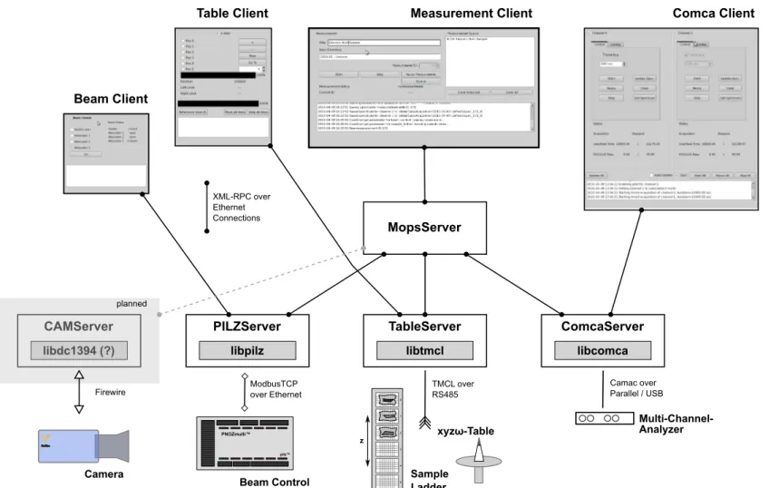
For the acquisition of the _γ -ray spectra a new automatic data-acquisition system has been developed during this work, which allows the consecutive measurement of all samples positioned in the vacuum chamber, with separately configurable beam properties and acquisition times, without the need for manual intervention. This system is described in chapter 3.4.3.

3.2. PGAI/NT setup at FRM 2

3.2.1. Modifications to the PGAA setup

For PGAI/NT measurements the configuration of the PGAA setup was changed:

• The _γ -collimator of detector 2 was exchanged by a lead collimator with signifi-

cantly smaller aperture (ch. 3.2.3).

Table 3.1.: Beam parameters of the PGAA setup at FRM 2 [Kud08a, Can09, Can10]

Beam parameter

mean neutron spectrum energy 1.83 meV mean neutron wavelength 6.7 Å

thermal equivalent neutron flux 2.42 · 10 ¹⁰ n/cm ² (no nose)

∼ 5.5 · 10 ¹⁰ n/cm ^2∗ (with nose) usable beam size (w × h) (14 × 38) mm (no nose)

(4 × 10) mm (with nose)

∗

Expected. Actual value currently under analysis (see [Can10]).

• The PGAA “sample ladder” and the vacuum chamber were removed to make space for the (x, y, z, _ω )-positioning table.

• A newly constructed CCD tomograph was placed behind the sample position for NT.

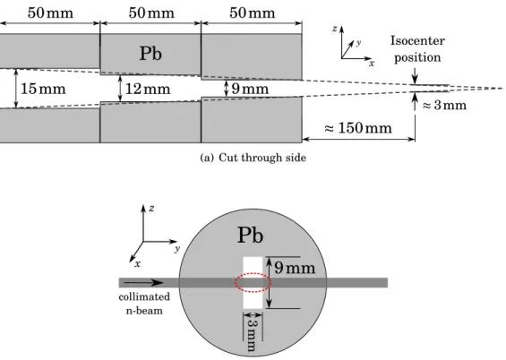
• For NT measurements the neutron flight path was prolonged by a 160 cm long, boron-shielded flight tube, to obtain a more parallel neutron beam at sample position. To improve the beam quality even further it proved to be effective to insert two boron collimator windows of about 3 × 5 cm ² into this flight tube to

“cut” away the most divergent neutrons.

• For PGAI measurements an adjustable neutron collimator was placed into the neutron beam (ch. 3.2.4).

During the measurement presented in this work the elliptical “nose” at the exit of the beam guide was not used despite the higher neutron fluxes it should deliver. The resulting beam with “nose” proved to be very divergent, which extremely influences the isovolume shape. Hence, these first measurements at the new PGAI/NT setup were performed with lower flux but a better defined isovolume.

The setup in PGAI/NT configuration and the layout of the measurement chamber are shown in figure 3.2. The features of the NT part of the configuration are exten- sively described in [Ebe09]. The properties of the PGAI part are investigated here.

3.2.2. Alignment of the PGAI/NT setup Necessity of a proper alignment

For an accurate position-sensitive imaging measurement a thorough alignment of the

measurement setup is indispensable. For PGAI measurements the alignment of the

neutron and _γ -collimator is the most crucial part. If the _γ -collimator’s field-of-view

does not cross the collimated neutron pencil beam, one will not be able to measure

anything or, if the alignment is not optimal, only with limited count-rates. That

1100 5800

62x28 18x8

110x50

Figure 3.1.: Cut through the PGAA setup at FRM 2

means one has to align two about 2–3 mm wide lines in a three-dimensional space of about (30 × 30 × 30) cm ³ to create an isovolume. In addition one has to determine the coordinates of this isovolume in units of motor steps of the (x, y, z, _ω )-moving table for correct sample positioning.

The following procedure for the alignment of a PGAI/NT setup has been produced from experiences and procedures developed at the Institutes of Isotopes of the Hun- garian Academy of Sciences in Budapest, where first tests of the new PGAI method were carried out [Bel08a, Bel08b, Sze08b], and extended by the experiences gained at the PGAI/NT setup at FRM 2.

Alignment procedure

The fixed axis for the alignment of the other equipment is the prolongation of the

neutron beam guide, which defines the flight path of the incoming neutrons. All other

equipment must be aligned to this line. The PGAI detector with the small _γ -collimator

is placed under a 90 ^◦ angle with respect to the neutron beam. Because the detector

should be heavily shielded by lead bricks, its position can be seen as “quasi”-fixed. A

fine adjustment of the _γ -collimator may not be possible, at least for the PGAI setup

at FRM 2, when the massive lead shielding is once in place. Thus, one has to align

the collimated neutron beam to hit the prolongation of the _γ -collimator, during the

(a) Setup in NT configuration (b) PGAI/NT measurement chamber Figure 3.2.: Setup in PGAI/NT configuration

alignment procedure. Taking these two lines as fixed the further alignment of the setup can be approached as follows:

Positioning of the neutron tomograph The neutron tomograph is an invaluable tool for the further procedure, thus one should position it in the beginning. Its exact positioning is not so important, but one should take care that it is posi- tioned quite perpendicular to the beam to avoid distortions in the radiographies, that it is close to the expected sample positions to avoid blurring in the radio- graphies, and that it covers the full expected sample area. It is helpful if the tomograph is fixed with respect to the setup, because one may then compare absolute pixel-positions in the radiographies for different sample positioning processes.

Alignment of the moving table ^{The (x, y,} z)-axes of the moving table are normally designed to be perpendicular to each other, thus the accuracy of their orienta- tion towards each other is defined by the quality of the moving table and cannot be influenced. Normally this accuracy should be sufficiently high. One axis of the table, in our case called y-axis, has now to be aligned to follow the neutron beam line. In lucky cases this line may be marked on the setup, which eases the process. Without such help one has to find other means to roughly align the table to this line.

For the fine alignment of the table orientation one may then use the open neu-

tron beam and the tomography system, by placing a thin calibration object on

the table. When this object is moved along the beam line, its position on the

tomograph’s scintillator should not change (or only very little). If the radiog-

raphy image of the object moves during this process, the table’s y-axis has to

be adjusted. This steps should be repeated until the orientation of the table is satisfying.

Adjustment of the table’s rotation ⁽ ω ) -axis The rotational orientation of the mov- ing table should be aligned in such a way that the sample support is orientated perpendicular to the beam for an angle of 0 ^◦ , giving a defined sample orienta- tion. Good moving tables may have reference switches, defining fixed position for the stepper motors. If this reference position for the rotational axis is in a known orientation to the (x, y)-axes probably no further alignment is necessary.

If this is not the case one may use again the neutron tomograph for alignment.

By placing a long, flat calibration object in a defined orientation on the moving table, the angle 0 ^◦ , i.e. parallel orientation of the object with respect to the beam, is reached when the thickness of the object’s projection on the neutron tomograph’s scintillator is minimal. This defines the fixed reference position of the _ω -axis.

Determination of the γ -collimator’s ^{( y, z)} -position A time consuming and tricky task is the exact localization of the _γ -collimator’s position in terms of motor steps. This process should be done in two steps: A coarse and a fine positioning of the moving table. As first step an intense _γ -source of minimal, point-like size is positioned in the center of rotation of the moving table. For a safer support it is advisable to fix the source on a larger object of known dimensions. Finally the γ -collimator position then has to be corrected for the height of this supporting object.

For the coarse positioning the most effective and fastest method showed also to be the easiest: The _γ -collimator is extended by sticking e.g. a long, straight wire into it, thus prolonging its line-of-view. The wire should be long enough to reach the middle of the measurement chamber. Afterwards the _γ -source is moved with the moving table in y- and z-directions to the position of the wire.

As result the source should now be quite near to the desired position in front of the _γ -collimator. Other methods, utilizing a precise alignment of a laser that is placed at the detector position and aims through the _γ -collimator into the measurement chamber, proved to be not as effective, because the laser beam gets reflected at the lead walls of the collimator. This produces reflection pat- terns inside the measurement chamber, which are hard to distinguish from an unreflected laser spot.

For the fine positioning one now performs a scan around the coarsely deter- mined isovolume position and measures the count-rates produced by the _γ - source. The position with the highest intensity rates identifies the motor po- sitions of the isovolume in y- and z-direction.

Positioning of the neutron collimator As a final step the neutron collimator has

to be positioned in that way, that the collimated neutron beam hits the previ-

ously determined y- and z-position of the isovolume. The x-coordinate can be

freely chosen with respect to other constrains like available space or practical positioning considerations. Anyhow, it is advisable to locate it quite close to the _γ -detector, to gain higher count-rates and a better spatial resolution for the measurements. On the other hand an isovolume very close to the _γ -detector may hinder the sample positioning, due to geometrical reasons. Another impor- tant aspect is the inhomogeneity of the neutron beam intensity. It is advisable to select a neutron collimator position with a high neutron flux, which can be determined with the help of the neutron tomograph. For an easier positing of the neutron collimator in the (important) z-direction a movable collimator, as introduced in chapter 3.2.4, proved to be useful.

Again the neutron tomography system is used for n-collimator positioning. One now puts a sharp, well defined calibration object, e.g. a small gadolinium dot on the tip of a metal cone, on the moving table and moves it into the previ- ously measured _γ -collimator position ( y _iso , z _iso ). With the help of the neutron tomograph the neutron collimator is now adjusted in height, until the small cal- ibration object is visible in its center. Now _γ - and neutron collimator form the desired isovolume.

General advice

The alignment process can be quite time consuming, but fortunately it only has to be done once, as long as the moving table does not “forget” its current positions, e.g. due to a power failure or due to lost motor steps. Precautions for such a case should be taken to avoid unnecessary work. As mentioned above good moving tables may pro- vide reference switches for a recalibration of the position values. Even better tables may have internal batteries that keep track of the current motor positions during a power failure. Encoders that count the actual motor steps eliminate the risk of lost steps. If these handy features are not available, one has to improvise, by defining spe- cial, easy reproducible positions on each table axis, and use these positions as origin for the alignment.

3.2.3. Design and properties of the γ -collimator Design

The first _γ -collimator was fabricated after a design suggested in [PC07], where Monte-

Carlo-simulations about the expected spatial resolutions with a 15 cm long lead col-

limator were made. That collimator featured a circular entry window of 2 mm di-

ameter, which was enlarged to 3 mm diameter for the last 5 cm. The result of the

simulations was an expected spatial resolution of about 3.8 mm for photons in the

range of 1000 keV–5000 keV. The spatial resolution is depending on the energy of

the photons, because higher energetic _γ -rays can penetrate deeper into the shielding

material and thus have a bigger likelihood of reaching the detector. Measurements

at the PGAA setup at the Budapest Research Reactor showed a spatial resolution of

about 4 mm – 6 mm for a square _γ -collimator of (2 × 2) mm ² [Bel07].

(a) Cut through side

(b) Front view with marked position of the isovolume.

Figure 3.3.: Sketch of the γ-collimator (not in scale), fabricated from three distinct lead pieces.

During the first test measurements at the PGAI/NT setup at FRM 2 it turned out that the _γ -count-rates with an collimator-aperture of only 2 mm diameter were too low for really effective measurements. Thus, the aperture was enlarged over the full length to 3 mm. To increase the count-rates even further, the height of the collimator window was enlarged in 3 steps, to 9 mm for the first 5 cm, 12 mm in the next 5 cm, and 15 mm for the last 5 cm interval. These increasing sections should mimic a tri- angular shape, which was not realized due to practical manufacturing reasons. The dimensions were chosen to maximize the number of passing _γ -rays, which are emit- ted radially from the isovolume, for an isovolume height of up to ≈ 3 mm (fig. 3.3(a)), while still blocking as much as possible from the _γ -ray background. Viewed from the front side the _γ -collimator has a rectangular shape, if we neglect minor deviations in the corners due to the drilling process used to produce the collimator.

As a reminder: The extended height should not decrease the measurement res-

olution in the z-axis direction, because only the volume irradiated by the confined

neutron beam is emitting _γ -rays (if we neglect neutron scattering effects inside the

sample; see chapter 3.2.4). The relevant parameter for the space resolution in z-

(and x)-direction is the size of the collimated neutron beam at isovolume position. The

γ -collimator just confines the depth of the isovolume, i.e. the y-direction (fig. 3.3(b)).

Measurement of the γ -collimator-resolution

To measure the spatial resolution and the intensity profile of the _γ -collimator, a ¹⁵² Eu calibration source was moved along the y- and z- axis in front of the collimator at a distance of about 10 cm. A rectangular area of ( ∆ y × ∆ z) = (8 × 18) mm ² , covering the upper half of the collimator’s slit, was scanned in 9 measurement steps in intervals of 1 mm in y-direction and 10 steps of 2 mm in z-direction. The peaks of five strong lines of ¹⁵² Eu, covering the energy region from 121.78 keV to 1408.01 keV have been analyzed at each position. The resulting peak areas have been normalized for each energy and plotted in a 9 × 20 grid in figure 3.5. One can clearly see from the plots that the effective area of the _γ -collimator is increasing for higher _γ -ray energies.

0 250 500 750 1000 1250 1500 1750

Energy / ^(keV)

5.5 6.0 6.5 7.0

R es ol ut io n / (m m )

Figure 3.4.: Resolution of the γ -collimator in dependence of the γ -ray energy, measured with a

Eu calibration source

The lowest line of the scanned grid was positioned to be at the height of the isocen- ter for the measurement, so the intensities at this line have been taken for the resolu- tion fit. For the measured intensities along this line we expect the following behavior:

• Far away from the collimator the intensity should be vanishing.

• Approaching the collimator aperture the intensities should start to increase.

Ideally one would like to have a sudden intensity jump from “0” to “1”, when

the sample crosses the border of the collimator’s slit.