A Simple Test on 2-Vertex- and 2-Edge-Connectivity

(1)

A Simple Test on 2-Vertex- and 2-Edge-Connectivity

Jens M. Schmidt

Max Planck Institute for Informatics

Abstract

Testing a graph on 2-vertex- and 2-edge-connectivity are two funda- mental algorithmic graph problems. For both problems, different linear- time algorithms with simple implementations are known. Here, an even simpler linear-time algorithm is presented that computes a structure from which both the 2-vertex- and 2-edge-connectivity of a graph can be easily

“read off”. The algorithm computes all bridges and cut vertices of the input graph in the same time.

1 Introduction

Testing a graph on 2-connectivity (i. e., 2-vertex-connectivity) and on 2-edge- connectivity are fundamental algorithmic graph problems. Tarjan presented the first linear-time algorithms for these problems, respectively [13, 14]. Since then, many linear-time algorithms have been given (e. g., [2, 3, 5, 6, 7, 8, 15, 16, 17]) that compute structures which inherently characterize either the 2- or 2-edge-connectivity of a graph. Examples include open ear decompositions [10, 18], block-cut trees [9], bipolar orientations [2] and s-t-numberings [2] (all of which can be used to determine 2-connectivity) and ear decompositions [10]

(the existence of which determines 2-edge-connectivity).

Most of the mentioned algorithms use a depth-first search-tree (DFS-tree) and compute the so-called low-point values, which are defined in terms of a DFS-tree (see [13] for a definition of low-points). This is a concept Tarjan introduced in his first algorithms and that has been applied successfully to many graph problems later on. However, low-points do not always provide the most natural solution: Brandes [2] and Gabow [8] gave considerably simpler algorithms for computing most of the above-mentioned structures (and testing 2-connectivity) by using simple path-generating rules instead of low-points; they call these algorithms path-based.

The aim of this paper is a self-contained exposition of an even simpler linear- time algorithm that tests both the 2- and 2-edge-connectivity of a graph. It is suitable for teaching in introductory courses on algorithms. While Tarjan’s two algorithms are currently the most popular ones used for teaching (see [8]

for a list of 11 text books in which they appear), in my teaching experience, undergraduate students have difficulties with the details of using low-points.

The algorithm presented here uses a very natural path-based approach in-

stead of low-points; similar approaches have been presented by Ramachan-

dran [12] and Tsin [16] in the context of parallel and distributed algorithms,

(2)

respectively. The approach is related to ear decompositions; in fact, it computes an (open) ear decomposition if the input graph has appropriate connectivity.

Notation. We use standard graph-theoretic terminology from [1]. Let δ(G) be the minimum degree of a graph G. A cut vertex is a vertex in a connected graph that disconnects the graph upon deletion. Similarly, a bridge is an edge in a connected graph that disconnects the graph upon deletion. A graph is 2-connected if it is connected and contains at least 3 vertices, but no cut ver- tex. A graph is 2-edge-connected if it is connected and contains at least 2 vertices, but no bridge. Note that for very small graphs, different definitions of (edge)connectivity are used in literature; here, we chose the common definition that ensures consistency with Menger’s Theorem [11]. It is easy to see that every 2-connected graph is 2-edge-connected, as otherwise any bridge in this graph on at least 3 vertices would have an end point that is a cut vertex.

2 Decomposition into Chains

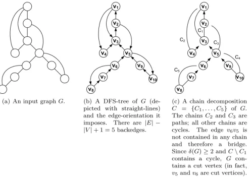
We will decompose the input graph into a set of paths and cycles, each of which will be called a chain. Some easy-to-check properties on these chains will then characterize both the 2- and 2-edge-connectivity of the graph. Let G = (V, E) be the input graph and assume for convenience that G is simple and that |V | ≥ 3.

This is not a severe restriction, as self-loops do not influence 2- or 2-edge- connectivity and can therefore be deleted in advance. Similarly, parallel edges do not influence 2-connectivity, but they may influence 2-edge-connectivity, as a bridge does not have parallel edges. However, the 2-edge-connectivity algorithm given in this paper still works for graphs with parallel edges.

We first perform a depth-first search on G. This implicitly checks G on being connected. If G is connected, we get a DFS-tree T that is rooted on a vertex r;

otherwise, we stop, as G is neither 2- nor 2-edge-connected. The DFS assigns a depth-first index (DFI) to every vertex. We assume that all tree edges (i. e., edges in T ) are oriented towards r and all backedges (i. e., edges that are in G but not in T ) are oriented away from r. Thus, every backedge e lies in exactly one directed cycle C(e).

Let every vertex be marked as unvisited. We now decompose G into chains by applying the following procedure for each vertex v in ascending DFI-order:

For every backedge e that starts at v, we traverse C(e), beginning with v, and stop at the first vertex that is marked as visited. During such a traversal, every traversed vertex is marked as visited. Thus, a traversal stops at the latest at v and forms either a directed path or cycle, beginning with v; we call this path or cycle a chain and identify it with the list of vertices and edges in the order in which they were visited. The ith chain found by this procedure is referred to as C

i

.

The chain C

1

, if exists, is a cycle, as every vertex is unvisited at the beginning (note C

1

does not have to contain r). There are |E| − |V | + 1 chains, as every one of the |E| − |V | + 1 backedges creates exactly one chain. We call the set C = {C

1

, . . . , C

_|E|−|V_|+1

} a chain decomposition; see Figure 1 for an example.

Clearly, a chain decomposition can be computed in linear time. This almost

concludes the algorithmic part; we now state easy-to-check conditions on C

(3)

(a) An input graphG.

v₁₀ v₄

v1

v6

v₅ v9

v₃ v2

v₇ v8

(b) A DFS-tree of G (de- picted with straight-lines) and the edge-orientation it imposes. There are |E| −

|V|+ 1 = 5 backedges.

C₄ C₃ C2

C₁

C5

v₁₀ v₄

v1

v6

v₅ v9

v₃ v2

v₇ v8

(c) A chain decomposition C = {C1, . . . , C5} of G.

The chainsC2 and C3 are paths; all other chains are cycles. The edge v6v5 is not contained in any chain and therefore a bridge.

Sinceδ(G)≥2 andC\C1

contains a cycle, G contains a cut vertex (in fact, v5andv6are cut vertices).

Figure 1: A graph G, its DFS-tree and a chain decomposition of G.

that characterize 2- and 2-edge-connectivity. All proofs will be given in the next section.

Theorem 1. Let C be a chain decomposition of a simple connected graph G.

Then G is 2-edge-connected if and only if the chains in C partition E.

Theorem 2. Let C be a chain decomposition of a simple 2-edge-connected graph G. Then G is 2-connected if and only if C

1

is the only cycle in C.

The properties in Theorems 1 and 2 can be efficiently tested: In order to check whether C partitions E, we mark every edge that is traversed by the chain decomposition. In order to check the property in Theorem 2, we check that C

₁

is a cycle and that, for every i > 1, the end vertices of C

_i

are distinct. For pseudo-code, see Algorithm 1.

Algorithm 1 Check(graph G) . G is simple and connected with |V | ≥ 3

1:

Compute a DFS-tree T of G

2:

Compute a chain decomposition C; mark every visited edge

3:

if G contains an unvisited edge then

4:

output “not 2 -edge-connected”

5:

else if there is a cycle in C different from C

1

then

6:

output “ 2 -edge-connected but not 2 -connected”

7:

else

8:

output “ 2 -connected”

We state a variant of Theorem 2, which does not rely on edge-connectivity.

Its proof is very similar to the one of Theorem 2.

(4)

Theorem 3. Let C be a chain decomposition of a simple connected graph G.

Then G is 2-connected if and only if δ(G) ≥ 2 and C

₁

is the only cycle in C.

3 Proofs

It remains to give the proofs of Theorems 1 and 2. For a tree T rooted at r and a vertex x in T , let T (x) be the subtree of T that consists of x and all descendants of x (independent of the edge orientations of T ). We will need the following well-known lemma (see, e.g., [4]).

Lemma 4. An edge is a bridge if and only if it is not contained in any cycle.

Theorem 1 is immediately implied by the following lemma.

Lemma 5. Let C be a chain decomposition of a simple connected graph G. An edge e in G is a bridge if and only if e is not contained in any chain in C.

Proof. Let e be a bridge and assume to the contrary that e is contained in a chain whose first edge (i. e., whose backedge) is b. According to Lemma 4, the bridge e is not contained in any cycle of G. This contradicts the fact that e is contained in the cycle C(b).

Now let e be an edge that is not contained in any chain in C. Let T be the DFS-tree that was used for computing C and let x be the end point of e that is farthest away from the root r of T , in particular x 6= r. Then e is a tree-edge, as otherwise e would be contained in a chain. For the same reason, there is no backedge with exactly one end point in T(x). Deleting e therefore disconnects all vertices in T (x) from r. Hence, e is a bridge.

The following lemma implies Theorem 2, as every 2-edge-connected graph has minimum degree 2.

Lemma 6. Let C be a chain decomposition of a simple connected graph G with δ(G) ≥ 2. A vertex v in G is a cut vertex if and only if v is incident to a bridge or v is the first vertex of a cycle in C \ C

1

.

Proof. Let v be a cut vertex in G; we may assume that v is not incident to a bridge. Let X and Y be connected components of G \ v. Then X and Y have to contain at least two neighbors of v in G, respectively. Let X

^+v

and Y

^+v

denote the subgraphs of G that are induced by X ∪ v and Y ∪ v, respectively.

Both X

^+v

and Y

^+v

contain a cycle through v, as both X and Y are connected.

It follows that C

1

exists; assume w. l. o. g. that C

1

∈ / X

^+v

. Then there is at least one backedge in X

^+v

that starts at v, since the DFS-tree is rooted in Y

^+v

and X

^+v

contains a cycle through v. When the first such backedge is traversed in the chain decomposition, every vertex in X is still unvisited. The traversal therefore closes a cycle that starts at v and is different from C

1

, as C

1

∈ / X

^+v

.

If v is incident to a bridge, δ(G) ≥ 2 implies that v is a cut vertex. Now let

v be the first vertex of a cycle C

i

6= C

1

in C. If v is the root r of the DFS-tree T

that was used for computing C, both cycles C

1

and C

i

end at v. Thus, v has at

least two children in T and v must be a cut vertex. Otherwise v 6= r; let wv be

the last edge in C

_i

. Then no backedge starts at a vertex with smaller DFI than

v and ends at a vertex in T (w), as otherwise vw would not be contained in C

_i

.

Thus, deleting v separates r from all vertices in T (w) and v is a cut vertex.

(5)

4 Extensions

We state how some additional structures can be computed from a chain de- composition. Note that Lemmas 5 and 6 can be used to compute all bridges and all cut vertices of G in linear time. Having these, the 2-connected compo- nents (i. e., the maximal 2-connected subgraphs) of G and the 2-edge-connected components (i. e., the maximal 2-edge-connected subgraphs) of G can be easily obtained: it suffices to cut the DFS-tree T along all cut-vertices or, respectively, all bridges. The former also gives the so-called block-cut tree [9] of G, which is a tree representing the dependency of the 2-connected components and cut vertices of G. Similarly, cutting all bridges in T gives a tree that represents the dependency of the 2-edge-connected components and bridges of G.

Additionally, the set of chains C computed by our algorithm is an ear de- composition if G is 2-edge-connected and an open ear decomposition if G is 2-connected. Note that C is not an arbitrary (open) ear decomposition, as it de- pends on the DFS-tree. The existence of these ear decompositions characterize the 2-(edge-)connectivity of a graph [10, 18]; Brandes [2] gives a simple linear- time transformation that computes a bipolar orientation and an s-t-numbering from such an open ear decomposition.

References

[1] J. A. Bondy and U. S. R. Murty. Graph Theory. Springer, 2008.

[2] U. Brandes. Eager st-Ordering. In Proceedings of the 10th European Symposium of Algorithms (ESA’02), pages 247–256, 2002.

[3] J. Cheriyan and K. Mehlhorn. Algorithms for dense graphs and networks. Algo- rithmica, 15(6):521–549, 1996.

[4] R. Diestel. Graph Theory. Springer, fourth edition, 2010.

[5] J. Ebert. st-Ordering the vertices of biconnected graphs. Computing, 30:19–33, 1983.

[6] S. Even and R. E. Tarjan. Computing an st-Numbering. Theor. Comput. Sci., 2(3):339–344, 1976.

[7] S. Even and R. E. Tarjan. Corrigendum: Computing an st-Numbering (TCS 2(1976):339-344). Theor. Comput. Sci., 4(1):123, 1977.

[8] H. N. Gabow. Path-based depth-first search for strong and biconnected compo- nents. Inf. Process. Lett., 74(3-4):107–114, 2000.

[9] F. Harary and G. Prins. The block-cutpoint-tree of a graph. Publ. Math. Debrecen, 13:103–107, 1966.

[10] L. Lovász. Computing ears and branchings in parallel. In Proceedings of the 26th Annual Symposium on Foundations of Computer Science (FOCS’85), pages 464–467, 1985.

[11] K. Menger. Zur allgemeinen Kurventheorie. Fund. Math., 10:96–115, 1927.

[12] V. Ramachandran. Parallel open ear decomposition with applications to graph biconnectivity and triconnectivity. In Synthesis of Parallel Algorithms, pages 275–340, 1993.

[13] R. E. Tarjan. Depth-first search and linear graph algorithms. SIAM Journal on

Computing, 1(2):146–160, 1972.

(6)