Pion distribution amplitude from lattice QCD

(1)

Pion distribution amplitude from lattice QCD

Jian-Hui Zhang,

^1,*

Jiunn-Wei Chen,

^2,3,†

Xiangdong Ji,

^4,5,‡

Luchang Jin,

^6,§

and Huey-Wen Lin

^7,8,∥

1

Institut für Theoretische Physik, Universität Regensburg, D-93040 Regensburg, Germany

2

Department of Physics, Center for Theoretical Sciences, and Leung Center for Cosmology and Particle Astrophysics, National Taiwan University, Taipei, Taiwan 106

3

Center for Theoretical Physics, Massachusetts Institute of Technology, Cambridge, Massachusetts 02139, USA

4

Tsung-Dao Lee Institute, and College of Physics and Astronomy, Shanghai Jiao Tong University, Shanghai 200240, People ’ s Republic of China

5

Maryland Center for Fundamental Physics, Department of Physics, University of Maryland, College Park, Maryland 20742, USA

6

Physics Department, Brookhaven National Laboratory, Upton, New York 11973, USA

7

Department of Physics and Astronomy, Michigan State University, East Lansing, Michigan 48824, USA

8

Department of Computational Mathematics, Science and Engineering, Michigan State University, East Lansing, Michigan 48824, USA

(Received 17 February 2017; published 31 May 2017)

We present the first lattice-QCD calculation of the pion distribution amplitude using the large- momentum effective field theory (LaMET) approach, which allows us to extract light cone parton observables from a Euclidean lattice. The mass corrections needed to extract the pion distribution amplitude from this approach are calculated to all orders in m

²π

=P

²z

. We also implement the Wilson-line renormalization which is crucial to remove the power divergences in this approach, and find that it reduces the oscillation at the end points of the distribution amplitude. Our exploratory result at 310-MeV pion mass favors a single-hump form broader than the asymptotic form of the pion distribution amplitude.

DOI: 10.1103/PhysRevD.95.094514

I. INTRODUCTION

Hadronic light cone distribution amplitudes (DAs) play an essential role in the description of hard exclusive processes involving large momentum transfer. They are crucial inputs for processes relevant to measuring funda- mental parameters of the Standard Model and probing new physics [1]. The QCD factorization theorem and asymp- totic freedom allow us to separate the short-distance physics incorporated in the hard quark and gluon subpro- cesses from the long-distance physics incorporated in the process-independent hadronic DAs. While the short- distance hard quark and gluon subprocesses are calculable perturbatively, the hadronic DAs are intrinsically non- perturbative. To determine them, we must resort to exper- imental measurements, lattice calculations or QCD models.

The simplest and most extensively studied hadronic DA is the twist-2 DA of the pion. It represents the probability amplitude of finding the valence q¯ q Fock state in the pion with the quark (antiquark) carrying a fraction x ( 1 − x ) of the total pion momentum. The pion light cone distribution amplitude (LCDA) is defined as

ϕ

π

ðxÞ ¼ i f

π

Z dξ

2π e

^{iðx−1Þξλ·P}

hπðPÞj ψ ¯ ð0Þλ

· γγ

₅

Γð0; ξλÞψðξλÞj0i ð 1 Þ with the normalization R

₁

0

dxϕ

π

ðxÞ ¼ 1 , where the two quark fields are separated along the light cone with λ

^μ

¼ ð1; 0; 0; −1Þ= ffiffiffi

p 2

, and x ( 1 − x ) denotes the momen- tum fraction of the quark (antiquark). The twist-2 pion DA can be constrained from experimental measurements of e.g.

the pion form factor [2], and then as an input can be used to test QCD in, for example, γγ → π

⁰

from BABAR and Belle Collaboratios [3,4]. Some experiments proposed [5] at J-PARC might also be of use. At large momentum transfer, the pion DA is well-known to follow a universal asymptotic form [6]: ϕ

π

ðx; μ → ∞Þ → 6xð1 − xÞ . However, there have been some debates over the shape of the pion DA at lower scales μ . For example, Ref. [7] suggested a “ double- humped ” shape for the pion DA, which is very different from the asymptotic form, while other QCD models (for example, large- N

c

Regge model [8], QCD sum rule calculations [9], Nambu-Jona-Lasinio model [10], Dyson- Schwinger equations [11], truncated Gegenbauer expan- sion [12], just to name a few) do not suggest such a feature.

Unfortunately, lattice calculations have traditionally only been able to extract the lowest few moments of the pion DA after using the operator product expansion (OPE). The highest moment ever calculated on the lattice is the second

*

jianhui.zhang@ur.de

†

jwc@phys.ntu.edu.tw

‡

xji@umd.edu

§

ljin.luchang@gmail.com

∥

hwlin@pa.msu.edu

(2)

moment [13 – 17], and most calculations struggled with the noise-to-signal ratio. Reference [18] took the moment results from lattice-QCD calculations and reconstructed the pion DA using a specific parametrization; however, the errors propagating from the lattice calculations are rela- tively large, preventing them from discriminating between the QCD models. Calculating moments beyond the lowest two on the lattice is much more difficult due to the breaking of rotational symmetry by discretization, which induces divergent mixing coefficients to lower moments such that the noise-to-signal becomes a big problem. It was proposed to use a smeared source to reduce the discretization error [19], or to use another scale to replace the lattice cutoff in the mixing. For example, by using a heavy-light current in the OPE for the current-current correlator, the scale in the mixing parameters is replaced by the heavy-quark mass [20] or the gradient-flow scale in the proposal of Ref. [21].

Having an alternative approach to calculate the pion DA with better precision and quantifiable systematics is highly desirable so that it can be used to make predictions in other harder-to-calculate processes, such as B → ππ .

Recently, a new approach has been proposed to calculate the full x dependence of parton quantities, such as parton distributions, distribution amplitudes, etc. [22]. The method is based on the observation that, while in the rest frame of the nucleon, parton physics corresponds to light cone correla- tions, the same physics can be obtained through time- independent spatial correlations in the infinite-momentum frame (IMF) of the hadron after a matching procedure. This has been incorporated into a large-momentum effective field theory (LaMET) [23]. According to the LaMET, for a given light cone observable such as the PDF or the DA, one can construct a time-independent quasiobservable which depends on the hadron momentum, but approaches the light cone observable if the infinite momentum limit is taken prior to a UV regularization. In practical lattice computations, what one calculates is the quasiobservable at large but finite hadron momentum with UV regularization imposed first.

The difference between the quasi- and light cone observable is just the order of limits. This is similar to an effective field theory setup. One can then convert the quasi observable to the light cone one through a factorization or matching formula [23] (there exist also other approaches to extract light cone quantities from Euclidean ones, see e.g. [24 – 28]).

There have been many studies on factorization [29] and determinations of the one-loop corrections needed to connect finite-momentum quasidistributions to light cone distributions for nonsinglet leading-twist PDFs [30], gen- eralized parton distributions (GPDs) [31], transversity GPDs [32] and pion DA [31] in the continuum. Reference [33] also explores the renormalization of quasidistributions, and establishes that the quasidistribution is multiplicatively renormalizable at two-loop order. There are also proposals to improve the quark correlators to remove linear divergen- ces in the one-loop matching [34], to improve the nucleon

source to get higher nucleon momenta on the lattice [35], and to use the nonperturbative evolution of quasidistributions as a guide for the extrapolation of lattice results at moderate momentum to infinite momentum [36,37]. In Refs. [38,39], it was shown that the power divergence present in the long- link matrix elements can be removed by a mass renormal- ization in the auxiliary z -field formalism, in the same way as the renormalization of power divergence for an open Wilson line. After the Wilson-line renormalization, the long-link matrix elements are improved such that they contain at most logarithmic divergences. A nonperturbative determination of the mass counterterm can, for example, be done following the procedure based on the static-quark potential for the renormalization of Wilson loop in Ref. [40].

The first attempts to apply the LaMET approach to compute parton observables were the direct lattice compu- tations of the unpolarized, helicity and transversity iso- vector quark distributions [41 – 46]. Although the current lattice systematics are not yet fully accounted for, a sea- flavor asymmetry has been qualitatively seen in both the unpolarized and linearly polarized cases, part of which has been confirmed in the updated measurements by the STAR [47] and PHENIX [48] Collaborations. The Drell-Yan experiments at FNAL (E 1027 þ E 1039 ) and future EIC data will be able to give more insight into the sea asymmetry in the transversely polarized nucleon.

In this paper, we present the first direct lattice-QCD results for the Bjorken- x dependence of the pion DA using lattice gauge ensembles with N

f

¼ 2 þ 1 þ 1 highly improved staggered quarks (HISQ) [49] (generated by the MILC Collaboration [50]) and clover valence fermions with pion mass 310 MeV. In the framework of LaMET, the pion LCDA ϕðxÞ can be studied from the IMF limit of the following quasi-distribution amplitude (quasi-DA) ϕðx;P ~

_z

Þ ¼ i

f

_π

Z dz

2π e

^{−iðx−1ÞP}^z^z

hπðPÞj ψð0Þγ ¯

^z

γ

₅

Γð0;zÞψðzÞj0i ð 2 Þ with the two quark fields separated along the spatial z direction. As shown in Ref. [31], the pion LCDA can be related to the quasi-DA by the following matching formula:

ϕðx; ~ Λ; P

z

Þ ¼ Z

₁

0

dyZ

ϕ

ðx; y; Λ; μ; P

z

Þϕðy; μÞ þ O

Λ

²_QCD

P

²z

; m

²π

P

²z

; ð 3 Þ

where Λ ¼ π=a is the UV cutoff for the quasi-DA with a the lattice spacing. μ denotes the MS renormalization scale ¯ of the pion LCDA. Using Eq. (3), we will be able to recover the pion LCDA.

The paper is organized as follows: We will start by

discussing the finite-momentum corrections for the quasi-

DA computed on the lattice in Sec. II and then present the

lattice results in Sec. III. We first show the results without

(3)

Wilson-line renormalization to remove the power diver- gence and then explore the impact of Wilson-line renorm- alization where the mass counterterm is determined by using the static-quark potential for the renormalization of Wilson loop discussed in Ref. [40]. Finally we summarize in Sec. IV . The details of the finite-momentum corrections are given in the Appendixes.

II. FINITE-P

_z

CORRECTIONS FOR PION QUASIDISTRIBUTION AMPLITUDE

In this section, we present the finite-momentum correc- tions needed for the calculation of pion DA. In the limit P

z

→ ∞, the matching becomes the most important P

z

correction. The factor Z

ϕ

has been computed up to one loop in Ref. [31] using a momentum-cutoff regulator instead of a lattice regulator. Therefore, this Z factor is accurate up to the leading logarithm but not for the numerical constant.

Determining this constant requires a calculation using lattice perturbation theory with the same lattice action.

At tree level, the Z

_ϕ

factor is just a delta function. Up to one-loop level, we can write

Z

_ϕ

ðx; yÞ ¼ δðx − yÞ þ α

_s

2π Z ¯

_ϕ

ðx; yÞ þ Oðα

²s

Þ; ð 4 Þ such that

ϕðxÞ ~ ≃ ϕðxÞ þ α

_s

2π

Z

dy Z ¯

ϕ

ðx; yÞϕðyÞ: ð 5 Þ Since the difference between ϕðxÞ ~ and ϕðxÞ starts at the loop level, we can rewrite the above equation as

ϕðxÞ ≃ ϕðxÞ ~ − α

s

2π Z

dy Z ¯

ϕ

ðx; yÞ ϕðyÞ ~ ð 6 Þ with an error of Oðα

²_s

Þ [29]. As in the parton distribution, Z ¯

_ϕ

ðx; yÞ can be written as

Z ¯

ϕ

ðx; yÞ ¼ ðZ

^ð1Þ_ϕ

ðx; yÞ − Cδðx − yÞÞ; ð 7 Þ with the first term coming from gluon emission and the second term from the quark self-energy diagram, C ¼ R

_∞

−∞

dx

⁰

Z

^ð1Þ_ϕ

ðx

⁰

; yÞ. [This implies R

dxϕðxÞ ¼ R

dx ϕðxÞ ~ at one loop, which follows from the conservation of the nonsinglet axial current when quark masses are neglected.]

Using this, Eq. (6) becomes ϕðxÞ ≃ ϕðxÞ ~ − α

_s

2π Z

_∞

−∞

dy½Z

^ð1Þ_ϕ

ðx; yÞ ϕðyÞ ~ − Z

^ð1Þ_ϕ

ðy; xÞ ϕðxÞ; ~ ð8Þ where for simplicity we have extended the integration range of y to infinity, which introduces an error at higher order.

The expression for the matching factor Z

^ð1Þ_ϕ

ðx; yÞ is given in Appendix A.

For a finite P

z

, we need to take into account the Oðm

²π

=P

²z

Þ meson-mass and OðΛ

²QCD

=P

²z

Þ higher-twist corrections. Following a procedure similar to Ref. [45], we can derive the mass corrections to all orders in m

²_π

=P

²_z

, which leads to the following relation between the pion DAs (for details see Appendix B):

ϕðxÞ ¼ ffiffiffiffiffiffiffiffiffiffiffiffiffi 1 þ 4c

p X

^∞

n¼0

ð4cÞ

ⁿ

f

^2nþ1þ

×

ð1 þ ð−1Þ

ⁿ

Þ ϕ ~ 1

2 − f

^2nþ1_þ

ð1 − 2xÞ 4ð4cÞ

ⁿ

þ ð1 − ð−1Þ

ⁿ

Þ ϕ ~ 1

2 þ f

^2nþ1þ

ð1 − 2xÞ 4ð4cÞ

ⁿ

; ð 9 Þ where c ¼ m

²π

=4P

²_z

and f

þ

¼ ffiffiffiffiffiffiffiffiffiffiffiffiffi

1 þ 4c

p þ 1.

The OðΛ

²_QCD

=P

²z

Þ correction can be derived in the same way as in Ref. [45], since the twist-4 operator involved is the same. The twist-4 effect can be implemented by adding a ϕ ~

_twist-4

contribution to ϕ ~ , such that

ϕðx; ~ Λ; P

z

Þ → ϕðx; ~ Λ; P

z

Þ þ ϕ ~

twist-4

ðx; Λ; P

z

Þ; ð 10 Þ where

ϕ ~

twist-4

ðx; Λ; P

z

Þ ¼ 1 8π

Z

_∞

−∞

dzΓ

0

ð−ixzP

z

ÞhπðPÞjO

tr

ðzÞj0i;

ð11Þ Γ

₀

is the incomplete Gamma function and

O

tr

ðzÞ¼ Z

z

0

dz

1

ψð0Þ½γ ¯

^ν

γ

5

Γð0;z

1

ÞD

ν

Γðz

1

;zÞ þ

Z

_z

1

0

dz

2

λ· γγ

₅

Γð0;z

₂

ÞD

^ν

Γðz

₂

;z

1

ÞD

_ν

Γðz

₁

;zÞψ ðzλÞ ð 12 Þ with λ

^μ

¼ ð0; 0; 0; −1Þ . Equations (8) – (10) take into account the one-loop, mass and higher-twist corrections, respectively.

We need to implement them step by step to achieve the final pion DA. For the higher-twist corrections, instead of com- puting them directly on the lattice, we only parametrize and fit them as a 1=P

²_z

correction after we have removed other leading- P

z

corrections, as was done in Ref. [45].

III. NUMERICAL RESULTS AND DISCUSSION

In this section, we report the first results of a lattice-QCD

calculation of the x -dependence of the pion DA. We use

clover valence fermions on gauge ensembles with 2 þ 1 þ

1 flavors (degenerate up/down, strange and charm degrees

of freedom in the QCD vacuum) of highly improved

staggered quarks (HISQ) [49] generated by MILC

Collaboration [50]. The pion mass of this ensemble is

m

_π

≈ 310 MeV with lattice spacing a ≈ 0 . 12 fm and box

size L ≈ 3 fm, corresponding to m

_π

L ≈ 4 . 5 . The HISQ

(4)

ensembles are hypercubic (HYP)-smeared [51] and the clover parameters are tuned to recover the lowest pion mass of the staggered quarks in the sea.

¹

HYP smearing has been shown to significantly improve the discretization effects on operators and shift their corresponding renormalizations toward their tree-level values (near 1 for quark bilinear operators). The results shown in this work are done using correlators calculated from three source locations on 986 configurations. For each positive z -momentum P

_z

, the matrix elements are averaged with their corresponding

−P

_z

to improve the signal.

A. Results from pion quasidistribution amplitude We begin with the pion quasi-DA without the Wilson-line renormalization, and then we follow similar steps to those listed in our previous work on nucleon parton distribution functions: First, we implement the one-loop and mass corrections whose formulas are detailed in the previous sections, and extrapolate to the infinite-momentum limit via αðxÞ þ βðxÞ=P

²z

[and thereby remove the higher-twist terms that come in at OðΛ

²_QCD

=P

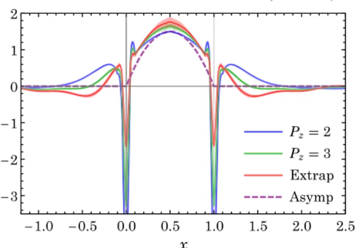
²_z

Þ ]. The true light cone pion DA should be recovered. Figure 1 shows the results for the pion DA at μ ¼ 2 GeV after implementing one-loop and mass corrections at different momenta P

_z

¼ 2 , 3 (in units of 2π=L ) to the quasi-DA.

²

We then extrapolate using these two momenta to the infinite-momentum limit using the form αðxÞ þ βðxÞ=P

²_z

, shown in red, where a linear divergence is present in the one-loop matching kernel (later, we will show improved results for the pion DAwhere the power divergence is removed by taking into account the Wilson-line normali- zation). The dashed line is the asymptotic form 6xð1 − xÞ . All our resulting curves are symmetric around x ¼ 1=2, as expected from the symmetry of the pion DA under the interchange x ↔ 1 − x . The pion DA has often been expanded in terms of Gegenbauer polynomials in past studies, and the dashed curve here contains only the zeroth Gegenbauer polynomial. The other three curves are broader than the asymptotic form, indicating contribution from higher Gegenbauer polynomials.

We note several interesting features of this result.

First, the pion DA is expected to vanish outside the region x ∈ ½0; 1 after taking the IMF limit. We see the P

_z

¼ 2 pion quasi-DA is nonzero for x ∈ ½1; 1.7, and this range shrinks to x ∈ ½1; 1 . 4 for P

z

¼ 3 . A similar pattern is observed for the region x < 0 . The distributions are moving in the right direction as the pion DA will vanish outside [0, 1]

with P

_z

→ ∞ . However, after taking the IMF limit via

extrapolation formula αðxÞ þ βðxÞ=P

²z

, we find there is still residual distribution outside x ∈ ½0; 1 . This is likely due to using the approximation Eq. (8), where the cancellation among ϕðxÞ ~ outside the x ∈ ½0; 1 region is between an all- order result and a perturbative expression, and is therefore incomplete

³

This can be improved by including the higher- order matching and going to larger momentum, which we will explore more extensively in future work.

Second, the results near x ¼ 0 and x ¼ 1 are not reliable.

There are unphysical peaks and dips due to the linear divergence in the one-loop matching in these regions, which become smaller as P

z

becomes larger. The small- est- x region is dominated by the smallest nonzero momen- tum fraction, which is proportional to 1=L (where L is the lattice length along boosted-momentum direction), due to the finite box size. To improve results near these regions would require large momentum and large box size.

Third, the unphysical oscillatory behavior near x ¼ 0 and x ¼ 1 is largely due to the presence of a linear divergence in the one-loop matching for the bare long-link matrix element. In Refs. [38,39], it has been shown that the power divergence (in the a → 0 limit) in the long-link operator can be removed to all orders by a mass counterterm δm (in the auxiliary z -field description of the Wilson line), which is the same as in the renormalization of an open Wilson line. After the Wilson-line renormalization, the pion quasi-DA is improved such that it contains at most logarithmic divergences. We will investigate this improved quasi-DA numerically in the rest of the paper.

FIG. 1. The pion distribution amplitude (at μ ¼ 2 GeV) after implementing one-loop and mass correction for P

z

¼ 2 (blue) and 3 (green) (in units of 2π=L ) to the quasidistribution amplitude. The extrapolation to infinite momentum to remove the remaining higher-twist effects is shown in red. The Wilson- line renormalization that removes the power divergent contribu- tion is not included in this plot and will be implemented later in the results of improved pion quasi-DA. The purple dashed line is the asymptotic form 6xð1 − xÞ .

1

Other studies using the same setup are done in Refs. [52 – 55], and no exceptional-configuration behavior was observed.

2

For this work, we initially calculate the pion quasi-DA for three momenta, P

z

¼ 1 , 2, 3 (in units of 2π=L ), but the corrections term for the smallest-momentum distribution is less well-behaved, as observed in the nucleon PDF case [45]; thus, we drop it in the rest of this work.

3

Although the difference here is formally of higher order, it

might have a sizable numerical effect.

(5)

B. Results from the improved pion quasidistribution amplitude

The improved pion quasi-DA without power divergence can be defined as [39]

ϕ ~

imp

ðx; P

z

Þ ¼ i f

π

Z dz

2π e

^{−iðx−1ÞP}^z^z−δmjzj

× hπðPÞj ψð0Þγ ¯

^z

γ

₅

Γð0; zÞψ ðzÞj0i; ð 13 Þ where δm should be determined nonperturbatively through studying the Wilson-line renormalization. It is worthwhile to comment that since the mass counterterm δm cancels all power divergence in the improved pion quasi-DA,

⁴

when we do the perturbative matching between Eqs. (13) and (1), we need to remove the linear divergence present in the one- loop matching kernel for consistency. Moreover, as shown in Ref. [39] and below, δm is negative, the exponential factor e

^−δmjzj

then increases the weight of matrix elements with relatively large z , and thereby increases the contribu- tion at relatively small momentum when Fourier trans- forming to momentum space. It is therefore important to properly account for the higher-twist corrections.

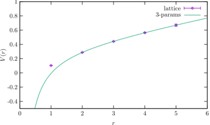
We first explore the nonperturbative determination of δm discussed in Ref. [40] using the static-quark potential for the renormalization of Wilson loop. The Wilson loop Wðt; rÞ of width r and length t is long in the t -direction such that higher excitations are sufficiently suppressed. The quark potential is then obtained as

VðrÞ ¼ − 1 a lim

t→∞

ln h Tr ½W ðt; rÞi

h Tr ½W ðt − a; rÞi ; ð14Þ where a is the lattice spacing and the cusp anomalous dimensions from the four sharp corners of the Wilson loop are canceled between numerator and denominator. When r is larger than the confinement scale but shorter than the string breaking scale,

⁵

the lattice data should be described by the energy of the static quark pairs

VðrÞ ¼ c

1

r þ c

₂

þ c

₃

r; ð 15 Þ where the c

₁

term is the Coulomb potential which domi- nates at short distance, c

₃

term is the confinement linear potential. The c

2

term is twice the rest mass of the heavy quark, and we expect c

2

¼ c=a ~ þ OðΛ

QCD

Þ . Thus, the δm counterterm that cancels the linear divergence in the Wilson line is

δm ¼ − c ~

2a ¼ − c

2

2 þ OðΛ

QCD

Þ: ð 16 Þ

This leads to

δm ≃ −260 200 MeV ; ð17Þ where we have used the fitted value δm ¼ −0 . 16=a from Fig. 2, which is 0.38 times of the one-loop value computed in Ref. [39], and we estimate the error by the size of Λ

QCD

∼ 200 MeV. The error can be reduced by performing the computation at different a to extract the 1=a -dependent term in c

₂

.

As mentioned before, once the improved pion DA of Eq. (13) is used with δm determined nonperturbatively, the linear divergence in the one-loop matching kernel will be canceled by the δm counterterm as shown in Eq. (A6). In Ref. [39], it was demonstrated that in the limit Λ=P

_z

→ ∞ , only the Wilson-line self-energy diagram is divergent among the “ real diagrams ” [i.e. Z

^ð1Þ_ϕ

ðx; yÞ of Eq. (7)] in one loop and in the Feynman gauge. Therefore, in a lattice perturbation theory calculation, one only needs to calculate this diagram, which is linearly divergent (∝ Λ=P

_z

). Using the simplest version of gauge-field discretization, one finds the matching between the momentum and lattice cutoffs is Λ ¼ π=a þ Oða

²

Þ . This result holds not only for the nonsinglet quasi-PDF operator used in Ref. [39], but also for the pion quasi-DA in this work. The “ virtual diagrams ” (i.e. C of Eq. (7) will contain logarithmic divergence from the quark self-energy diagram, which can be removed by adding counterterms in the lattice action or treating t he integration limits of C carefully. In Eq. (A6), the Λ=P

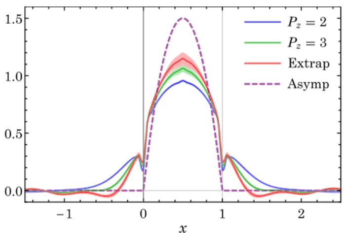
z

→ ∞ limit is not taken, so C is finite. We find that the difference between taking this limit and not is small, certainly within the error induced by the uncertainty of δm . The resulting pion DA using the improved pion quasi- DA of Eq. (13) with the central value of δm is shown in Fig. 3. The unphysical oscillations near x ¼ 0 and x ¼ 1 are largely removed. There are still small kinks in the unphysical region, but they are expected to vanish when

FIG. 2. The energy of the static-quark pairs fit to the functional form of Eq. (15). The point at r ¼ 1 is excluded from the fit to reduce discretization error. If we further exclude the r ¼ 2 point, then c

2

is increased by 15%, still in the range of Eq. (17).

4

At perturbative one-loop, it appears as a linear divergence, but more-divergent power divergences can appear at higher loops.

5

The onset of string breaking can be estimated by

VðrÞ > 2m

B

− m

Υ

¼ 1 . 1 GeV.

(6)

higher-order matching is taken into account and the P

z

→ ∞ limit is approached.

The final result that includes the lattice statistical uncertainties, finite- P

z

corrections and the uncertainty of δm estimated in Eq. (17) is presented in Fig. 4. Also shown in the same figure are the model calculation from the Dyson-Schwinger equation (DSE) [11], from the truncated Gegenbauer expansion fit to the Belle data for the γγ

→ π

⁰

form factor [12] and from parametrizations of the pion DA with the parameters fit to lowest-moment calculations from lattice QCD in [13]. For the fit to the Belle data, we use the Gegenbauer polynomial expansion up to the eighth moment given in Ref. [12] and run to 2 GeV. For the fit to the lattice moment calculations, we have chosen two

different parametrizations. One is simply a truncation of the Gegenbauer polynomial expansion of the pion DA to the second order ϕðxÞ ¼ 6xð1 − xÞ½1 þ a

2

C

³⁼²₂

ð2x − 1Þ (labeled “Param 1”) with the value of a

2

taken from [13].

The other is ϕðxÞ ¼ A½xð1 − xÞ

^B

with A and B determined from the normalization condition and the second moment of the pion DA (labeled “ Param 2 ” ). The second para- metrization is close to the DSE result, but differs from the first parametrization. The difference between them can be viewed as a rough estimate of errors from the truncation and reflects uncertainties in the parametrization, which are currently underestimated even though both bands have smaller errors than ours. A direct calculation of the x -dependence will help to resolve such uncertainties. Of course, this can be achieved only when the direct calcu- lation reaches a sufficiently high accuracy, which is difficult at the current stage but might be improved in the foreseeable future. Nonetheless, the results of our direct calculation at 310-MeV pion mass is in agreement within errors with DSE, Belle data fit result and the parametrized reconstruction of pion DAs in the region near x ¼ 1=2 , although the two parametrized forms differ from each other.

The uncertainty of our distribution is dominated by the δm uncertainty, which can be largely removed by performing calculations at different lattice spacing. As before, we still have residual distribution outside the [0, 1] region, which should vanish when larger momenta are reached and higher-order matching is taken into account in the future.

Also, as is typical in an exploratory study, the pion mass in this work is still heavier than its physical value. However, the study of Ref. [56] shows that the leading chiral correction for ϕ

_π

ðxÞ is proportional to m

²_π

with the chiral logarithm m

²_π

ln m

²_π

completely absorbed by f

_π

. This property will simplify the chiral extrapolation in future computations. It is encouraging that our current result is qualitatively similar to other determinations using lattice- moment parametrization, models and fits to experimental data, and also favors a single-hump distribution in ϕ

_π

ðxÞ .

IV. SUMMARY AND OUTLOOK

In this work, we presented the first lattice-QCD calculation of the pion distribution amplitude using the large-momentum effective field theory (LaMET) approach. We derived the mass-correction formulation needed for the pion quasidis- tribution amplitude. We also implemented the Wilson-line renormalization in this work, which is important to remove the power divergences in LaMET approach, and found that it reduces the oscillation at the end points of the distribution amplitude. Finally, our result at 310-MeV pion mass shows similar behavior as previous studies done using DSE, a fit to the Belle data and as parametrizations with latest lattice moment result, and favors a single-hump structure.

However, in the current study, we have not accounted for all possible systematic uncertainties, and there are multiple FIG. 3. Pion distribution amplitude at μ ¼ 2 GeV derived from

the improved pion quasidistribution amplitude of Eq. (13) and δm ¼ 0 . 38δm

1-loop

in Eq. (13) for P

z

¼ 2 (blue) and 3 (green) (in units of 2π=L ) and extrapolation to infinite-momentum limit (red), along with the asymptotic form 6xð1 − xÞ (dashed line).

FIG. 4. Pion distribution amplitude at μ ¼ 2 GeV with δm ¼

ð0 . 38 0 . 28Þδm

1-loop

(red band with the central value denoted by

red dot-dashed) obtained in this work (labeled as “ LaMET ” ),

along with that obtained from the Dyson-Schwinger equation

(labeled “ DSE ” ) analysis of the pion (blue), a fit to the Belle

data (labeled “ Belle ” , cyan), parametrized fits to the lattice

moments (labeled “ Param 1 ” and “ Param 2 ” , respectively, gray

and green) and the asymptotic form (labeled “ Asymp ” , purple).

(7)

improvements that can be done in future studies. For example, in our work, it is clear that larger boosted momentum is needed for the pion distribution amplitude to make the result outside the physical region consistent with 0 than for the unpolarized nucleon parton distribution function. Finer lattice spacing would help reduce the uncer- tainty in the counterterm determined by the Wilson-loop study. Larger lattice box and also higher-order matching would reduce the unphysical kinks near x ¼ 1 and 0. Last but not least, we hope this work will encourage following works to extensively study the distribution amplitude of the pion and other hadrons.

ACKNOWLEDGMENTS

JHZ thanks G. Bali, V. Braun, and M. Göckeler and A.

Schäfer for valuable discussions and comments. The LQCD calculations were performed using the Chroma software suite [57]. We thank MILC Collaboration for sharing the lattices used to perform this study. Computations for this work were carried out in part on facilities of the USQCD Collaboration, which are funded by the Office of Science of the U.S.

Department of Energy, and on the National Energy Research Scientific Computing Center, a DOE Office of Science User Facility supported by the Office of Science of the U.S.

Department of Energy under Contract No. DE-AC02- 05CH11231. This work was partially supported by the U.S. Department of Energy via Grant No. DE-FG02- 93ER-40762, a grant (Grant No. 11DZ2260700) from the Office of Science and Technology in Shanghai Municipal

Government, grants from National Science Foundation of China (Grants No. 11175114, No. 11405104, No. 11655002), a DFG grant SCHA 458/20-1, the SFB/

TRR-55 grant “ Hadron Physics from Lattice QCD ” , the MIT MISTI program, the Ministry of Science and Technology, Taiwan under Grants No. 105-2112-M-002-017-MY3 and No. 105-2918-I-002 -003 and the CASTS of NTU. The work of JWC and XJ is supported in part by the U.S. Department of Energy, Office of Science, Office of Nuclear Physics, within the framework of the TMD Topical Collaboration. L. C. J. is supported by the Department of Energy, Laboratory Directed Research and Development (LDRD) funding of BNL, under Contract No. DE-SC0012704.

APPENDIX A: ONE-LOOP MATCHING FOR QUASI-DA OF PION

In this appendix, we list the one-loop matching factors used throughout this paper. These factors have been obtained in Ref. [31]. However, as in Ref. [45], we keep a finite cutoff Λ and do not take the limit Λ ≫ xP

_z

.

For the pion distribution amplitude, expanding the matching factor Z

_ϕ

ðx; y; Λ; μ; P

_z

Þ in Eq. (3) as

Z

ϕ

ðx;y; Λ;μ;P

z

Þ ¼ δðx− yÞþ α

S

2π Z

^ð1Þ_ϕ

ðx;y; Λ;μ;P

z

Þþ;

ð A1 Þ we have

Z

^ð1Þ_ϕ

ðx; y; Λ; μ; P

_z

Þ=C

_F

¼ G

1

ðx; y; Λ; μ; P

_z

Þθðx < 0Þ þ G

2

ðx; y; Λ; μ; P

_z

Þθð0 < x < yÞ

þ G

₃

ðx; y; Λ; μ; P

_z

Þθðy < x < 1Þ þ G

₄

ðx; y; Λ; μ; P

_z

Þθðx > 1Þ ð A2 Þ with

G

₁

ðx; y; Λ; μ; P

_z

Þ ¼ 1

x − y þ Λðx; 1Þ − Λðx; yÞ

2P

_z

ð1 − yÞðx − yÞ þ Λðx; yÞ − Λðx; 0Þ

2P

_z

ðx − yÞy þ Λðx; yÞ þ Λðy; xÞ 2P

_z

ðx − yÞ

²

þ

1 x − y − x 1 − y

ln ð1 − xÞ þ

1 x − y þ 1 − x y

ln ð−xÞ þ x

1 − y − 1 − x

y − 2

x − y

ln ðy − xÞ − 1 − x

2y þ 1 2ðx − yÞ

ln Λð0; xÞ Λðx; 0Þ þ

x

2ð1 − yÞ − 1 2ðx − yÞ

ln Λð1; xÞ Λðx; 1Þ þ

x

2ð1 − yÞ − 1 − x 2y − 1

x − y

ln Λðx; yÞ Λðy; xÞ ; G

₂

ðx; y; Λ; μ; P

_z

Þ ¼ 3

2y þ 1

2ðy − 1Þ − 2

y − x þ Λðx; 0Þ

2P

z

ðy − xÞy þ Λðx; 1Þ

2P

z

ð1 − yÞðx − yÞ þ ðx þ y − 2xyÞðΛðx; yÞ þ Λðy; xÞÞ 4P

_z

ðx − yÞ

²

yð1 − yÞ þ

x − 1

y þ 1

y − x

ln P

²z

μ

²

þ x − 1

y þ 1

y − x

lnð4xÞ þ x

y − 1 − 1 y − x

lnð1 − xÞ

þ x − 1

y þ 2

y − x − x y − 1

ln ðy − xÞ − 1

2y þ 1 2ðx − yÞ

ln Λð0; xÞ Λðx; 0Þ þ

x

2ð1 − yÞ − 1 2ðx − yÞ

ln Λð1; xÞ Λðx; 1Þ þ x

y ln Λðx; yÞ Λðx; 0Þ þ

x

2ð1 − yÞ − 1 2y − 1

x − y

ln Λðx; yÞ Λðy; xÞ ; G

3

ðx; y; Λ; μ; P

z

Þ ¼ G

2

ð1 − x; 1 − y; Λ; μ; P

z

Þ;

G

₄

ðx; y; Λ; μ; P

_z

Þ ¼ G

₁

ð1 − x; 1 − y; Λ; μ; P

_z

Þ; ð A3 Þ

where Λðx; yÞ ¼ ffiffiffiffiffiffiffiffiffiffiffiffiffiffiffiffiffiffiffiffiffiffiffiffiffiffiffiffiffiffiffiffi Λ

²

þ ðx − yÞ

²

P

²z

p þ ðx − yÞP

z

.

(8)

Near x ¼ y , one has an extra contribution from the quark wave function renormalization

Z

^ð1Þ_ϕ

ðx; y; Λ; μ; P

z

Þ=C

F

¼ δZ

^ð1Þ_ϕ

ð2π=α

S

Þδðx − yÞ; ð A4 Þ where δZ

^ð1Þ_ϕ

provides a plus prescription for the factor in Eq. (A2) and can be written as

δZ

^ð1Þ_ϕ

¼ Z

dxZ

^ð1Þ_ϕ

ðx; y; Λ; μ; P

_z

Þ: ðA5Þ If one used the improved pion DA of Eq. (13) for the computation, then the G

_i

function in the matching kernel will be replaced by

G

i

ðx;y; Λ;μ;P

z

Þ → G

i

ðx;y;Λ; μ;P

z

Þ− Λ

P

z

ðx−yÞ

²

: ð A6 Þ

APPENDIX B: MESON MASS CORRECTION FOR QUASI-DA OF PION

In this appendix, we derive the meson-mass corrections to the quasi-DA of the pion. For the pion DA, we need to calculate the same series sum as for the unpolarized parton distribution in Ref. [45],

K

n

¼ hð1 − 2xÞ

ⁿ⁻¹

i

ϕ~

hð1 − 2xÞ

ⁿ⁻¹

i

_ϕ

¼ X

ⁱ^max

i¼0

C

ⁱ_n−i

c

ⁱ

¼ λ

ðμ₁

λ

μ_nÞ

P

^μ¹

P

^μⁿ

λ

μ1

λ

μ_n

P

^μ¹

P

^μⁿ

;

ð B1 Þ

where c ¼ m

²π

=4P

²z

and ð…Þ means the indices enclosed are symmetric and traceless. The result for even n ( ¼ 2k ) is X

^k

j¼0

C

^j_n−j

c

^j

¼ ffiffiffiffiffiffiffiffiffiffiffiffiffi 1 1 þ 4c p

f

−

2

_2kþ1

þ f

þ

2

_2kþ1

; ðB2Þ while for odd n ( ¼ 2k þ 1 ), it is

X

^k

j¼0

C

^j_n−j

c

^j

¼ ffiffiffiffiffiffiffiffiffiffiffiffiffi 1 1 þ 4c p

− f

₋

2

_2kþ2

þ f

_þ

2

_2kþ2

; ð B3 Þ

where f

¼ ffiffiffiffiffiffiffiffiffiffiffiffiffi 1 þ 4c

p 1 .

With Eqs. (B2) and (B3), we perform an inverse Mellin transform on the moment relation of Eq. (B1)

1 2πi

Z

_i∞

−i∞

dns

⁻ⁿ

hð1 − 2xÞ

ⁿ⁻¹

i: ð B4 Þ To extract ϕðxÞ from ϕðxÞ ~ , let us rewrite Eq. (B1) for an even n ¼ 2k as

hð1 − 2xÞ

^2k−1

i

_ϕ

¼ hð1 − 2xÞ

^2k−1

i

ϕ~

ffiffiffiffiffiffiffiffiffiffiffiffiffi 1 þ 4c p

ð

^f₂⁻

Þ

^2kþ1

þ ð

^f₂^þ

Þ

^2kþ1

¼ hð1 − 2xÞ

^2k−1

i

_q_~

ffiffiffiffiffiffiffiffiffiffiffiffiffi 1 þ 4c p

ð

^f₂^þ

Þ

^2kþ1

× X

^∞

n¼0

ð−1Þ

ⁿ

f

−

f

þ

_ð2kþ1Þn

: ð B5 Þ

The inverse Mellin transform then leads to

ϕðxÞ − ϕð1 − xÞ ¼ 2 ffiffiffiffiffiffiffiffiffiffiffiffiffi 1 þ 4c

p X

^∞

n¼0

ð−f

₋

Þ

ⁿ

f

^nþ1_þ

ϕ ~ 1

2 − f

^nþ1þ

ð1 − 2xÞ 4f

ⁿ₋

− ϕ ~ 1

2 þ f

^nþ1þ

ð1 − 2xÞ 4f

ⁿ₋

: ð B6 Þ

Similarly, we have

ϕðxÞ þ ϕð1 − xÞ ¼ 2 ffiffiffiffiffiffiffiffiffiffiffiffiffi 1 þ 4c

p X

^∞

n¼0

f

ⁿ₋

f

^nþ1þ

ϕ ~ 1

2 − f

^nþ1_þ

ð1 − 2xÞ 4f

ⁿ₋

þ ϕ ~

1 2 þ f

^nþ1_þ

ð1 − 2xÞ 4f

ⁿ₋

: ð B7 Þ

Therefore,

ϕðxÞ ¼ ffiffiffiffiffiffiffiffiffiffiffiffiffi 1 þ 4c

p X

^∞

n¼0

f

ⁿ−

f

^nþ1_þ

ð1 þ ð−1Þ

ⁿ

Þ ϕ ~ 1

2 − f

^nþ1þ

ð1 − 2xÞ 4f

ⁿ₋

þ ð1 − ð−1Þ

ⁿ

Þ ϕ ~ 1

2 þ f

^nþ1þ

ð1 − 2xÞ 4f

ⁿ₋

¼ ffiffiffiffiffiffiffiffiffiffiffiffiffi 1 þ 4c

p X

^∞

n¼0

ð4cÞ

ⁿ

f

^2nþ1_þ

ð1 þ ð−1Þ

ⁿ

Þ ϕ ~ 1

2 − f

^2nþ1_þ

ð1 − 2xÞ 4ð4cÞ

ⁿ

þ ð1 − ð−1Þ

ⁿ

Þ ϕ ~ 1

2 þ f

^2nþ1_þ

ð1 − 2xÞ 4ð4cÞ

ⁿ

; ð B8 Þ

where in the last line we have used f

_þ

f

₋

¼ 4c . Since f

_þ

≫ f

₋

or c and the quasi-DA ϕðxÞ ~ vanishes asymptotically for

large x , the above sum is dominated by the first term with n ¼ 0 . In practical calculations, we can reach reasonable accuracy

by taking only the first few terms in the sum. In Refs. [58,59], it was argued that for hadron-to-vacuum matrix elements, the

mass corrections also receive contributions from higher-twist operators that can be reduced to total derivatives of twist-two

ones. We do not explicitly consider such terms, since they will anyway be part of the higher-twist corrections that are

parametrized with a specific form in the present work.

(9)