JHEP08(2019)065
Published for SISSA by Springer
Received: March 26, 2019 Revised: June 7, 2019 Accepted: June 30, 2019 Published: August 12, 2019
Light-cone distribution amplitudes of pseudoscalar mesons from lattice QCD
Gunnar S. Bali,a,b Vladimir M. Braun,a Simon B¨urger,a Meinulf G¨ockeler,a
Michael Gruber,a Fabian Hutzler,a Piotr Korcyl,c Andreas Sch¨afer,a Andr´e Sternbeckd and Philipp Weina on behalf of the RQCD collaboration
aInstitut f¨ur Theoretische Physik, Universit¨at Regensburg, 93040 Regensburg, Germany
bDepartment of Theoretical Physics, Tata Institute of Fundamental Research, Homi Bhabha Road, Mumbai 400005, India
cMarian Smoluchowski Institute of Physics, Jagiellonian University, ul. Lojasiewicza 11, 30-348 Krak´ow, Poland
dTheoretisch-Physikalisches Institut, Friedrich-Schiller-Universit¨at Jena, 07743 Jena, Germany
E-mail: gunnar.bali@ur.de,vladimir.braun@ur.de,simon.buerger@ur.de, meinulf.goeckeler@ur.de,michael1.gruber@ur.de,fabian.hutzler@ur.de, piotr.korcyl@uj.edu.pl,andreas.schaefer@ur.de,
andre.sternbeck@uni-jena.de,philipp.wein@ur.de
Abstract: We present the first lattice determination of the two lowest Gegenbauer mo- ments of the leading-twist pion and kaon light-cone distribution amplitudes with full control of all errors: aπ2 = 0.101+24−24 for the pion;aK1 = 0.0533+34−35 and aK2 = 0.090+19−20 for the kaon.
The calculation is carried out on 35 different CLS ensembles with Nf = 2 + 1 flavors of dynamical Wilson-clover fermions. These cover a multitude of pion and kaon mass combi- nations (including the physical point) and 5 different lattice spacings down toa= 0.039 fm.
The momentum smearing technique and a new operator basis are employed to reduce sta- tistical fluctuations and to improve the overlap with the ground states. The results are obtained from a combined chiral and continuum limit extrapolation that includes three separate trajectories in the quark mass plane.
Keywords: Lattice QCD, Nonperturbative Effects, Kaon Physics ArXiv ePrint: 1903.08038
JHEP08(2019)065
Contents
1 Introduction 1
2 General formalism 4
2.1 Continuum definitions 4
2.2 Lattice definitions 5
2.3 Renormalization procedure 7
3 Details of the lattice analysis 10
3.1 Lattice ensembles 10
3.2 Analysis of correlation functions 11
3.3 Chiral extrapolation 12
3.4 Discretization effects 14
4 Extrapolation strategy and error budget 15
4.1 A game of ones 15
4.2 Extrapolation of the second LCDA moments 16
4.3 Extrapolation of the first LCDA moment 18
4.4 Summary of the results 18
5 Discussion 20
A Lattice ensembles and supplementary figures 25
1 Introduction
Hadron light-cone distribution amplitudes (LCDAs) have been introduced four decades ago [1–7] in the context of the QCD description of hard exclusive reactions. The LCDAs are scale-dependent nonperturbative functions that can be interpreted as quantum-mechanical amplitudes. Within this article we will use the term “LCDAs” synonymous with the leading-twist LCDAs. The latter describe the distribution of the longitudinal momentum amongst the quarks in the leading Fock state contribution of a hadron wave function at small transverse parton separations. The pion LCDA is both the simplest LCDA and also the most important one in phenomenological applications. Unsurprisingly, it has received the most attention in the literature. Its precise knowledge is becoming increasingly relevant in flavor physics (where weak decays, such as B → π`ν`, B → ππ, etc., are providing information on the Cabibbo-Kobayashi-Maskawa matrix), in two-photon hard reactions (likeγ∗→γπ orγγ →ππ), and — as a tool to access the flavor separation in the nucleon generalized parton distributions — in hard exclusive electro-production (eN →eN π) with Bjorken kinematics.
JHEP08(2019)065
Theoretical attempts to predict the shape of the pion LCDA φπ(x, µ2) as a func- tion of the longitudinal momentum fraction x at a scale µ have a long history. The discussion was shaped for many years by the famous paper by Chernyak and Zhitnit- sky (CZ) [8] who calculated the second moment in x of the pion LCDA using QCD sum rules [9] and found a number much larger than the result expected at asymptotically large scales. Based on this calculation, CZ proposed a particular model for the pion LCDA at low scales, known as the CZ model. Assuming the validity of perturbative QCD factor- ization, this model allowed for a consistent description of all experimental data on hard exclusive processes that were available at that time [10]. In figure 1 we compare the asymptotic LCDA φπ(x, µ2)−−−→µ→∞ 6x(1−x) [4, 5] with the CZ model. The latter cor- responds to a double-peaked distribution, where one of the constituents is most likely to carry a small (∼ 0.15) and the other one a large (∼ 0.85) fraction of the longitudinal pion momentum.
The CZ model received some criticism. On the one hand, the validity of collinear factorization in hard exclusive reactions at relatively low momentum transfer was ques- tioned [11, 12] and the role of a competing “soft” or “end-point” mechanism was em- phasized. In particular it was shown [12, 13] that the data on the pion form factor at Q2 ∼ 1–3 GeV2 could be described by the soft contribution alone, without any “hard”
corrections. On the other hand, it was argued that the QCD sum rules employed in ref. [8]
were not reliable as they may suffer from large contributions from operators of higher dimension. A model for such higher-order contributions using the concept of nonlocal vac- uum condensates [14] yielded a much smaller value of the second moment than the CZ model, see ref. [15] for a state-of-the-art study. Finally, the explicit calculation [16] of the value of the pion LCDA at the mid-point x = 12, using an at that time novel method, the light-cone sum rule (LCSR) technique, gave a rather large number, see figure 1, inconsis- tent with the pronounced “dip” of the CZ model. Using the LCSR approach it was also shown for many examples, see, e.g., refs. [17–25], that the CZ model leads to very large soft contributions to hard reactions, which contradict the data. Nevertheless, the paradigm
“asymptotic-like LCDA versus CZ-like LCDA” continues to be the preferred language of many model studies.
A new wave of interest in the pion LCDA was inspired by the BaBar measurement [26]
of the pion transition form factorγγ∗→π that indicates very strong scaling violations up to the highest virtualities Q2 ∼ 40 GeV2 available. In order to explain this behavior, an unconventional “constant” shape of the pion LCDA was proposed [27,28], which triggered further discussion, see, e.g., ref. [22]. Although the similar Belle experiment [29] does not suggest strong scaling violations, the problem is far from being resolved and this measure- ment will be repeated by Belle II at the upgraded SuperKEKB accelerator at KEK [30]
with a much improved projected precision. Motivated by these experimental needs and in the absence of a convincing first-principles calculation, the pion LCDA continues to attract a lot of attention. In the last few years several new calculations appeared, most notably using techniques based on Dyson-Schwinger equations (DSE) [31]. A short overview of several existing models and their distinctive features can be found in ref. [32]. For further models see, e.g., refs. [33,34].
JHEP08(2019)065
0.0 0.2 0.4 x 0.6 0.8 1.0
0.00 0.25 0.50 0.75 1.00 1.25 1.50 1.75 2.00
φπ(x)
Figure 1. Models for the pion LCDA: the blue line shows the asymptotic shape corresponding to the limitµ→ ∞, while the orange line depicts the CZ model [8,10] for µ= 0.5 GeV. The green point shows the QCD light-cone sum rule result [16] for the mid-point atµ= 1 GeV.
Within the past 10–20 years lattice QCD has firmly established itself as the method of choice for nonperturbative calculations in QCD, as it has the potential to provide quanti- tative results with full control over all sources of uncertainty. The problem that we address here, however, is not simple. Lattice calculations of moments of the pion LCDA were pro- posed more than 30 years ago [35,36]. First pioneering studies were carried out within the quenched approximation in refs. [36–39] and withNf = 2 Wilson fermions in ref. [40]. The first modern calculations were performed more than a decade ago by the QCDSF/UKQCD collaboration usingNf = 2 nonperturbatively improved Wilson fermions [41] and somewhat later by RBC/UKQCD [42] as part of their Nf = 2 + 1 domain-wall fermion phenomenol- ogy program. More recently, the study of ref. [41] was extended in ref. [43] to a larger set of lattice ensembles with different volumes, lattice spacings, and pion masses down to mπ = 150 MeV, also implementing several technical improvements. In this way the er- rors due to the chiral extrapolation could be brought under control but still no controlled continuum limit extrapolation could be carried out.
In this paper we close this last gap and present results of the first lattice calculation of the two lowest moments of the pion and kaon light-cone distribution amplitudes with full control of all systematic errors. This progress has become possible by the CLS (Coordinated Lattice Simulations) community effort [44] aiming at the production of very fine lattices using open boundary conditions in time and further algorithmic improvements to reduce the autocorrelations within the Monte-Carlo time-series. (Autocorrelations increase as the continuum limit is approached.) The calculation reported in this work has been carried out on 35 ensembles (see appendixAfor details) usingNf = 2 + 1 flavors of nonperturbatively improved Wilson (clover) fermions with pion masses down to the physical point, employing 5 different lattice spacings down to a = 0.039 fm. In addition, we use the momentum smearing technique [45], which enables us to reduce statistical fluctuations by improving the overlap of the meson interpolating field with the ground state. Employing this technique, first results for the second moment of the pion LCDA for a single lattice spacing were reported in ref. [46]. Since then we have enlarged the operator basis (cf. also ref. [47]) and
JHEP08(2019)065
added four lattice spacings as well as other quark mass combinations. The results are then obtained pursuing combined chiral and continuum limit extrapolations, utilizing data from three separate trajectories in the quark mass plane. As a by-product we also obtain the continuum limit quark mass dependence of the LCDA moments. A similar determination of the wave function normalization constants and the first LCDA moments of the lowest-lying baryon octet can be found in the companion article [48].
This article is organized as follows. In section 2 we first introduce LCDAs as well as the operators and correlators used in our analysis. Next, the renormalization of the lattice matrix elements is explained. This includes two steps: nonperturbative renormalization in the RI0/SMOM (or RI0/MOM) scheme and perturbative conversion from this scheme to the MS scheme. In section 3 we describe the set of gauge ensembles employed. Subsequently, we detail the analysis of the correlation functions (including the specific choice of operators and external momenta) and extract the relevant matrix elements from the lattice. We also provide the extrapolation formulae for the quark mass and lattice spacing dependence.
Finally, in section 4, we present our results for the LCDA moments and assess the error budget, before we discuss our findings and confront these with values from the literature in section 5.
2 General formalism
2.1 Continuum definitions
Each pseudoscalar meson has only one independent leading-twist LCDA,φM, which can be defined via a meson-to-vacuum matrix element of a renormalized nonlocal quark-antiquark light-ray operator,
h0|¯q(z2n)[z2n, z1n]/nγ5u(z1n)|M(p)i=ifM(p·n) Z 1
0
dx e−i(z1x+z2(1−x))p·nφM(x, µ2), (2.1) where we consider the pion (M = π+) with ¯q = ¯d and the kaon (M = K+) with ¯q = ¯s.
Here, z1,2 are real numbers, nµ is an auxiliary light-like (n2 = 0) vector, and |M(p)i represents the ground state meson M with on-shell momentum p2 = m2M. The light-like Wilson line connecting the quark fields, [z2n, z1n], is inserted to secure gauge invariance.
The scale dependence ofφM is indicated by the argumentµ2. We denote the quark masses asmq.
Neglecting the isospin breaking due to electromagnetic effects and nondegenerate light quark masses (by setting mu =md ≡m`), the LCDAs of all (charged and neutral) pions are trivially related such that it is sufficient to consider only one representative; the same holds for the kaons. The decay constant fM appearing in eq. (2.1) can be obtained as the matrix element of a local operator,
h0|¯q(0)γ0γ5u(0)|M+(p)i=ifMp0, (2.2) and has the valuefπ ≈130 MeV [49] for the pion andfK ≈156 MeV [50] for the kaon.
JHEP08(2019)065
Within eq. (2.1) a fraction x of the longitudinal meson momentum is carried by the u quark, while the ¯q antiquark carries the remaining fraction 1−x. The difference of the momentum fractions is usually denoted as
ξ =x−(1−x) = 2x−1. (2.3)
The complete information on the LCDA can be encoded in a set of moments. One such set is defined by
hξniM(µ2) = Z 1
0
dx(2x−1)nφM(x, µ2). (2.4) Another possible set of moments is
aMn(µ2) = 2(2n+ 3) 3(n+ 1)(n+ 2)
Z 1 0
dx Cn3/2(2x−1)φM(x, µ2), (2.5) where Cn3/2(ξ) are Gegenbauer polynomials, which correspond to irreducible representa- tions of the collinear conformal group SL(2,R). Both sets, the ξ-moments hξni and the Gegenbauer moments aMn , are related by a simple linear transformation, cf. eqs. (2.15b) and (2.16b) below.1 Since the Gegenbauer polynomials form a complete set of functions, the LCDAs can be expanded as
φM(x, µ2) = 6x(1−x)
1 +
∞
X
n=1
aMn(µ2)Cn3/2(2x−1)
, (2.6)
where the coefficientsaMn are renormalized multiplicatively in leading logarithmic order as a consequence of conformal symmetry [51]. Due to C-parity, all odd moments of the pion, i.e., hξniπ and aπn forn= 1,3, . . ., vanish in the limit of exact isospin symmetry. Higher- order contributions in the Gegenbauer expansion are suppressed at large scales, since the anomalous dimensions of aMn increase with n [5]. Hence, in the asymptotic limit µ → ∞ only the leading term survives,
φM(x, µ2 → ∞) =φas(x) = 6x(1−x), (2.7) which is usually referred to as the asymptotic LCDA. From here on we will suppress the explicit scale dependence of the DAs and their moments in the notation. Our lattice results will be given at the fixed scale µ= 2 GeV in the MS scheme with three active flavors.
2.2 Lattice definitions
From now on we will work in Euclidean spacetime and follow the conventions of ref. [43].
The renormalized light-ray operator on the left-hand side of eq. (2.1) generates renormalized local operators. This means that the moments (2.4) of the LCDAs can be expressed in terms of matrix elements of local operators that can be evaluated using lattice QCD. In
1Note that the secondξ-moment is given by a matrix element of an operator that contains two deriva- tives, which, in the case of parton distributions, would be relevant for the determination of the third Mellin moment.
JHEP08(2019)065
order to calculate the first and second moments of the pseudoscalar LCDAs we define the bare lattice operators
P(x) = ¯q(x)γ5u(x), (2.8a)
Aρ(x) = ¯q(x)γργ5u(x), (2.8b)
Oρµ−(x) = ¯q(x)D⃗(µ−D⃖(µ
γρ)γ5u(x), (2.8c)
Oρµν− (x) = ¯q(x)D⃗(µD⃗ν −2D⃖(µD⃗ν+D⃖(µD⃖ν
γρ)γ5u(x), (2.8d) Oρµν+ (x) = ¯q(x)D⃗(µD⃗ν + 2D⃖(µD⃗ν+D⃖(µD⃖ν
γρ)γ5u(x), (2.8e) where the covariant derivative Dµ is discretized symmetrically. To obtain a leading-twist projection we symmetrize over all Lorentz indices and subtract all traces. This procedure is indicated by parentheses, e.g., O(µν) = 12(Oµν+Oνµ) − 14δµνOλλ. In principle, one could also consider an operatorOρµ+, replacing the minus sign in eq. (2.8c) by a plus sign.
However, as O+ρµ differs in C-parity from O−ρµ, these two operators cannot mix with each other so that Oρµ+ is irrelevant for our calculation. In contrast, the operator O+ρµν has the same C-parity as Oρµν− and must be taken into account. Introducing the shorthand notationD⃡µ=D⃗µ−D⃖µ, the operator Oρµν− can also be written as ¯q(x)D⃡(µD⃡νγρ)γ5u(x) in the continuum.
On a hypercubic lattice, the continuous O(4) symmetry is reduced to its discrete H(4) subgroup. This symmetry breaking can in principle induce mixing of the operators of interest with lower-dimensional operators accompanied by coefficient functions that diverge with a power of 1/a. For the first two ξ-moments this mixing can be avoided by selecting lattice operators that belong to a suitable irreducible representation of the hypercubic group H(4) [41, 42]. For the calculation of the first moment we use the operators O−4µ, while for the second moments we choose O±ρµν with all three indices different, see also section 2.3.
In order to extract the desired moments we use two-point correlation functions of the operators with an interpolating current,
Cρ(t,p) =a3X
x
e−ip·xhAρ(x, t)Pp†(0)i, (2.9a) Cρµ−(t,p) =a3X
x
e−ip·xhOρµ−(x, t)Pp†(0)i, (2.9b) Cρµν± (t,p) =a3X
x
e−ip·xhOρµν± (x, t)Pp†(0)i, (2.9c) where the indexpindicates that the quarks appearing within the interpolator (2.8a) have been momentum smeared [45,46] (employing APE smeared [52] spatial gauge transporters) to optimize the overlap with the ground state. The smearing parameters are not only adjusted according to the momentum but also optimized with respect to lattice spacing and quark mass. The ground state will dominate for sufficiently large values of the source- sink separationt. In this limit, neglecting effects from the temporal boundaries, one obtains
CO(t,p) = 1
2Eh0|O(0)|M(p)ihM(p)|Pp†(0)|0ie−Et, (2.10)
JHEP08(2019)065
with the ground state energyE=
√
m2M+p2. For ensembles with open boundaries in time we place the source and sink within a window where the exponentially suppressed boundary effects can be neglected and translational invariance in time is restored within statistical accuracy. Regarding ensembles with the conventional anti-periodic fermionic boundary conditions in time, one should include a second exponential, e−Et7→e−Et+τOτPe−E(T−t), where the sign factors τO, τP represent the transformation properties of O and P under time reversal.
For the extraction of the first moment we consider the ratios R−1,a = i
3
3
X
j=1
1 pj
C4j−(t,p)
C4(t,p) , R−1,b= 4E 3E2+p2
C44−(t,p)
C4(t,p) . (2.11a–b) Similarly, for the required matrix elements for the second moment we consider
R±2,a
1 =−1 3
3
X
i,j=1 i<j
1 pipj
C4ij± (t,p)
C4(t,p) , R±2,a
2 = 1 3
3
X
i=1
pi p1p2p3
C123± (t,p)
Ci(t,p) . (2.12a–b) In contrast to the ratios (2.11), the two ratios defined in eqs. (2.12) transform according to the same irreducible representation of H(4) and will give the same resultR2±=R2,a± 1 =R±2,a2 (in the limitt→ ∞,pj a−1). However,R±2,a1 andR±2,a2 are affected differently by excited states, cf. section 3.2.
2.3 Renormalization procedure
The lattice operators have to be renormalized to obtain matrix elements in the MS scheme.
As mentioned above, the continuous Euclidean O(4) symmetry is reduced to that of its finite hypercubic subgroup H(4) on the lattice. Therefore, symmetry imposes much weaker constraints on the mixing of operators under renormalization. In order to avoid mixing as far as possible, in particular mixing with lower-dimensional operators, we use operators from suitably chosen multiplets that transform according to irreducible representations of H(4) and possess a definite C-parity. In the case of the operators (2.8c) with one deriva- tive we consider two multiplets transforming according to nonequivalent representations:
one, labeled a, consisting of the six operators Oρµ− with 1 ≤ µ < ρ ≤4 and another one, labeled b, consisting of O44− and two further linear combinations of O11−, O22−, O−33, O−44. These do not mix with any other operators.
The operators (2.8d) and (2.8e) with two derivatives have equal C-parity and behave identically under both continuum and lattice spacetime transformations. Hence, they will necessarily mix with each other. We utilize the multiplets
O+423, O413+ , O+412, O123+ (2.13a) and
O−423, O413− , O−412, O123− , (2.13b) which transform under H(4) according to one and the same four-dimensional irreducible representation. Their symmetry properties guarantee that they do not mix with any other operators.
JHEP08(2019)065
We determine the renormalization and mixing coefficients nonperturbatively on the lattice using the same RI0/SMOM scheme [53] as was used in ref. [43]. For the coarser lattice spacings (β = 3.4,3.46,3.55) we have ensembles with different quark mass values m` =ms and (anti-)periodic boundary conditions in time at our disposal so that we can proceed in exactly the same way as in ref. [43], starting from Landau-gauge-fixed three- point functions
a12 V
X
x,y,z
e−ip·x−i(q−p)·z+iq·yhd(x)O(z)¯u(y)i, (2.14) where O represents the operators from eqs. (2.8b)–(2.8e) with an antiquark flavor ¯q = ¯d that is mass-degenerate with theu quark. However, a problem arises on the finer lattices.
For β = 3.7 and 3.85 we are forced to work with open boundary conditions in time to reduce autocorrelations in the Monte-Carlo time-series [54,55]. In this case we modify the computation of the required three-point functions in two respects: we place the momentum sources within a subvolume, keeping a sufficiently large distance from the boundaries in the time direction, and we restrict the (final) sum overzto an even smaller volume inside this subvolume. The further analysis can then be performed as in the periodic case. A detailed discussion, including a justification of this method and a comparison with the results from periodic boundary conditions, will be the topic of a dedicated, forthcoming publication.
The ensembles with symmetric quark masses (m`=ms) used for the calculation of the renormalization factors are detailed in table 8. Unfortunately, we could only afford to generate ensembles for two distinct values of m` =ms at β = 3.7 and 3.85. In the other cases the mass dependence of the amputated three-point functions is rather mild, so that we are confident that this restriction does not significantly affect the reliability of the required chiral extrapolations.
In the case of the first LCDA moment of the kaon it is also possible to carry out the renormalization via the RI0/MOM scheme [56,57], where even the three-loop matching to the MS scheme is available [58–60]. Therefore, we choose to present four distinct results:
with one- and two-loop matching [61, 62] via the RI0/SMOM scheme as well as with two- and three-loop matching using the RI0/MOM scheme.
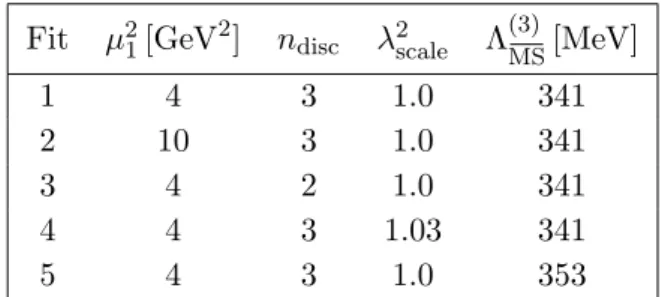
The tiny statistical errors of the results are negligible in comparison to the systematic uncertainties. In order to estimate the latter we proceed similarly to ref. [43] and per- form a number of fits, varying one element of the analysis at a time. We carry out two independent determinations of the renormalization and mixing coefficients, namely with one-loop and two-loop truncations of the perturbative expansion of the conversion factors from the RI0/SMOM scheme to the MS scheme for use in NLO and NNLO calculations in perturbative QCD, respectively. In both cases we vary the initial scale µ1 of the fit range and the number ndisc of terms in the parametrization A1a2µ2 +· · ·+Andisc(a2µ2)ndisc of the lattice artifacts. In order to take into account the uncertainties in the determination of the lattice spacing, the central values of 1/a2 shown in table1 are multiplied by a fac- torλ2scale = 1.03. This value contains the scale uncertainty of 8t∗0 =µ∗ −2ref given in ref. [63]
and the largest error of our determination of t∗0/a2, added in quadrature. Finally, also Λ(3)
MS= 341(12) MeV [63] is varied within its uncertainty. Thus, we end up with five types of fits; the different settings are compiled in table 2.
JHEP08(2019)065
β a[fm] 1/a2[GeV2] 3.40 0.086 5.28 3.46 0.076 6.75 3.55 0.064 9.44 3.70 0.050 15.75 3.85 0.039 25.54
Fit µ21[GeV2] ndisc λ2scale Λ(3)
MS[MeV]
1 4 3 1.0 341
2 10 3 1.0 341
3 4 2 1.0 341
4 4 3 1.03 341
5 4 3 1.0 353
Table 1. Lattice spacings. Table 2. Fit choices regarding the determination of the renormalization factors.
We determine the LCDA moments separately for each of the resulting renormalization and mixing coefficients, thus generating a set of five values per renormalization scheme at a given loop order. In this way we obtain two sets of results for the second LCDA moments, one using the two-loop SMOM conversion factors and another one employing the one-loop SMOM conversion factors. As explained above, for the first moment of the kaon LCDA we even have four such sets of results, as we can also nonperturbatively convert the bare lattice results to the RI0/MOM scheme instead and then utilize the two-loop or three-loop conversion factors between the RI0/MOM and the MS schemes.
In each set we take the results of fit 1 as our central values. Defining δi,i= 2,3,4,5, as the difference between the number based on fitiand the result based on fit 1, we estimate the systematic uncertainties due to the renormalization factors as
√
δ22+δ32+δ42+δ52. The dominant uncertainties are related to the low-momentum cut-off of our fit range (δ2), i.e., the scale dependence, and the parametrization of lattice artifacts (δ3). The former becomes smaller when going from one-loop to two-loop perturbative accuracy, while the latter uncertainty shrinks as the lattice spacing is reduced. The uncertainty induced by the scale setting (δ4) and the error of the strong coupling parameter (δ5) are negligible. Note that all figures in this article showing renormalized data are generated using the RI0/SMOM intermediate scheme with two-loop matching to the MS scheme.
Finally, the renormalized first moments are related to the ratios defined in eqs. (2.11) by hξ1iMS=ζaR−1,a =ζbR−1,b, aMS1 = 5
3hξ1iMS, (2.15a–b) while the second moments are related to the ratios (2.12) via
hξ2iMS=ζ11R−2 +ζ12R+2 , aMS2 = 7 12
5hξ2iMS− h12iMS
, (2.16a–b)
h12iMS=ζ22R+2 . (2.16c)
In the continuum h12iMS= 1, while it can differ from unity on the lattice, see section 4.1.
The ζs denote ratios of the renormalization constants of the operators (2.8c)–(2.8e) over the renormalization constant of the axialvector current (2.8b), cf. ref. [43]. Henceforth, hξni, h1ni, and an are always implied to be renormalized in the MS scheme and we omit the superscript MS.
JHEP08(2019)065
3 Details of the lattice analysis
3.1 Lattice ensembles
We use lattice ensembles generated within the CLS effort [44] employingNf = 2 + 1 flavors of nonperturbatively O(a) improved Wilson fermions [64,65] combined with the tree-level Symanzik improved gauge action [66]. For details on the action and the simulation see ref. [44].2 Since that publication more CLS simulation points have been added, see, e.g., ref. [68]. An overview of the ensembles analyzed here is given in appendix A. Most CLS ensembles use open boundary conditions in the time direction, which allows us to carry out simulations at very fine lattice spacings without facing the problem of topological charge freezing [54,55].
Five values of the inverse coupling constant β = 6/g2 are realized, corresponding to lattice spacings ranging from a = 0.086 fm down to a = 0.039 fm, see table 1. Here we set the scale using √
8t∗0 = 0.413(6) fm [63], where t∗0 is defined in ref. [69] as the Wilson flow scale t0 [70], computed at a particular reference point in the quark mass plane. The numerical value was obtained by matching the average continuum limit pion and kaon decay constantfπK = (2fK+fπ)/3 to experiment [69].
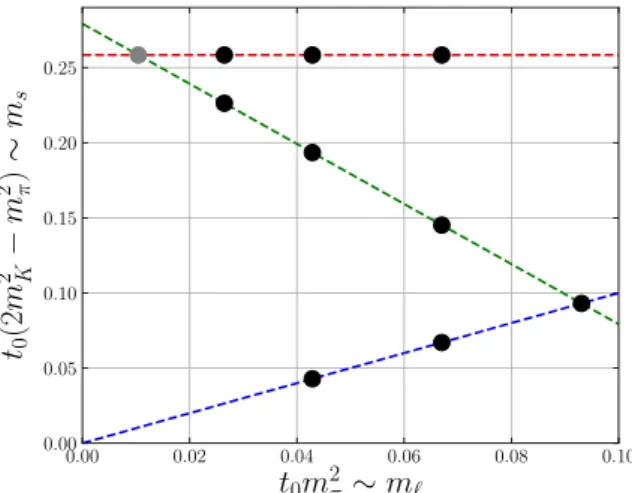
At each lattice spacing we have several points in the quark mass plane, along three trajectories: (a) along a nearly-physical fixed value of the trace of the mass matrix TrM ≡ mu+md+ms= 2m`+ms= phys., (b) varying the light quark mass while trying to keep the renormalized strange quark mass ms constant at its physical value, and (c) along the
“symmetric” line m` =ms, where light and strange quark masses are equal. The first two trajectories intersect close to the physical quark mass point. The locations of these three lines are shown in figure 2. We determine the LCDA moments on various ensembles along these trajectories; our largest pion mass is about 420 MeV and the smallest one is 130 MeV.
Table6 of appendix A contains all lattices lying on line (a) (TrM= constant). This line starts with a lattice at the flavor symmetric point and approaches the physical point, decreasing the light quark mass while simultaneously increasing the strange quark mass.
Table 7 contains all lattices lying on line (b) (ms ≈ constant), where the strange quark mass is fixed to its physical value. This line starts with lattices that have unphysically large values of the u and d quark mass m` and approaches the physical point with decreasing light quark mass. Finally, table 8contains all lattices on the SU(3)-symmetric line where m` =ms. Along this line, which also includes the symmetric point of the TrM= constant trajectory, all pseudoscalar mesons are members of a mass-degenerate SU(3) multiplet and their properties are related by symmetry.
The spatial extents of the lattices used to determine the LCDA moments are always larger than 2.4 fm and, with very few exceptions, larger than four times the inverse mass of the lightest pseudoscalar meson, see also tables6–8. For the pseudoscalar meson masses the expected corrections due to finite volume effects calculated at next-to-leading order in chiral perturbation theory (ChPT) [71,72] are smaller than half of their statistical errors.
2Some of them`=msensembles with (anti-)periodic boundary conditions in time have been generated by RQCD using the BQCD code [67].
JHEP08(2019)065
0.00 0.02 0.04 0.06 0.08 0.10
t0m2π∼m 0.00
0.05 0.10 0.15 0.20 0.25
t0(2m2 K−m2 π)∼ms
Figure 2. Schematic illustration of the mass trajectories of the lattice ensembles used in this study.
Along the flavor symmetric line (blue) all pseudoscalar mesons have equal mass (m2K =m2π), which is equivalent to equal quark masses (m=ms). The (green) line of the physical average quadratic meson mass (2m2K +m2π = phys.) corresponds to an approximately physical mean quark mass (2m+ms≈phys.). The red line is defined by 2m2K−m2π = phys. and indicates an approximately physical strange quark mass (ms≈phys.). The gray dot marks the physical point.
To this order the LCDAs are not affected by finite volume corrections at all since they are normalized with respect to the decay constant, see eq. (2.1). Therefore, it is well justified to neglect volume effects in our analysis.
3.2 Analysis of correlation functions
Below we specify our choice of correlators and momentum directions. For the first moment we have operators from two different H(4) multiplets at our disposal (cf. eqs. (2.11)).
For the ratio in eq. (2.11a) we select the momenta p = (±1,0,0)℘, p = (0,±1,0)℘, and p= (0,0,±1)℘, where℘= 2πL. We then extractR1,a− as a function of taccording to
R−1,a = i 3℘
3
j=1
pˆ−C4j−(t, ℘ej)
pˆ+C4(t, ℘ej) , (3.1) where the forward/backward momentum averaging is performed by the operator ˆp±:
pˆ±C(t,p) = 12
C(t,p)±C(t,−p)
. (3.2)
For the ratio in eq. (2.11b) we may simply set p=0 to obtain R−1,b= 4
3mK
C44−(t,0)
C4(t,0) . (3.3)
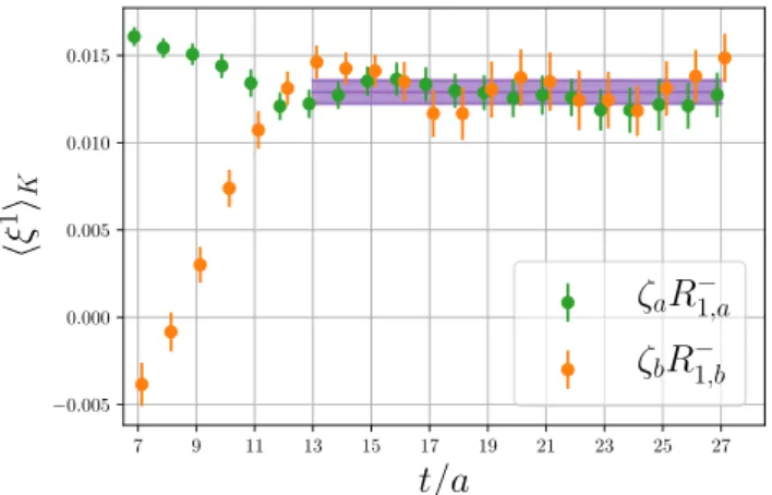
We then renormalize the above ratios, multiplying by ζa and ζb according to eq. (2.15a).
Finally, ξ1K is obtained by carrying out a simultaneous fit to the plateau that is reached at larget-values as depicted in figure3.
JHEP08(2019)065
7 9 11 13 15 17 19 21 23 25 27
t/a
−0.005 0.000 0.005 0.010 0.015
ξ1 K
ζaR−1,a ζbR1,b−
Figure 3. The ratios corresponding to the renormalized momentξ1Kdefined in eqs. (3.1) and (3.3) as a function of the timetin lattice units for the example of ensemble J501 witha= 0.039 fm. The result of a combined fit to both ratios is depicted in purple.
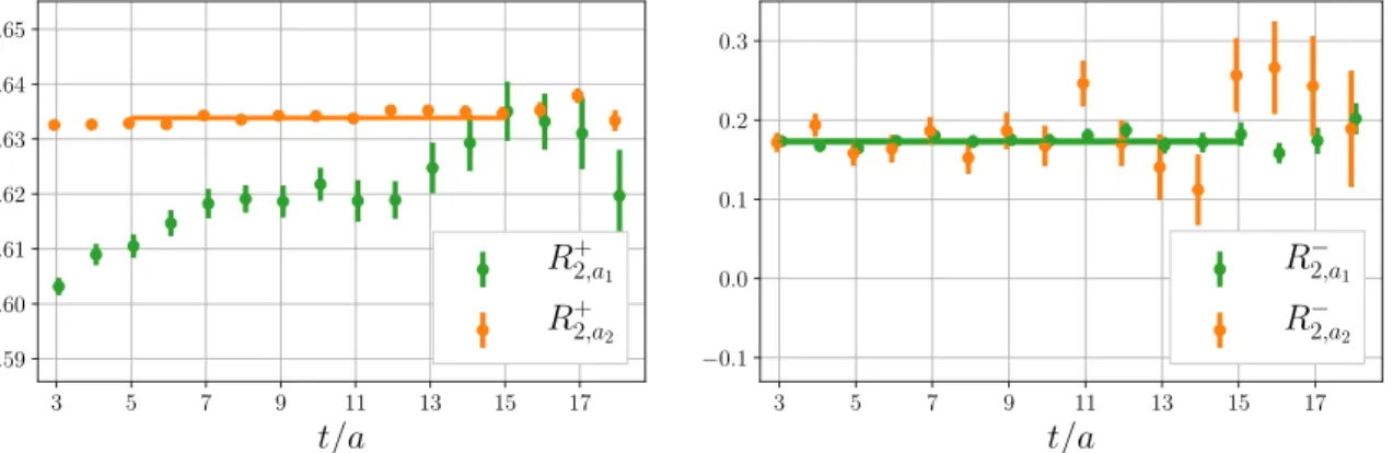
For the extraction of the second moments one needs at least two nonvanishing momen- tum components, cf. eqs. (2.12). We have already addressed the problem of the deteriora- tion of the signal-to-noise ratio for increasing momenta|p|in our previous work [46], where we proposed to employ the momentum smearing technique (introduced in ref. [45]) for all quark sources in order to improve the statistical error and to reduce contributions from excited states. The momentum smearing technique requires two inversions per momentum direction and in order to evaluate the full sum in eq. (2.12a) we performed six inversions to realize the momenta p = (1,1,0)℘, p = (1,0,1)℘, and p = (0,1,1)℘ in ref. [46]. In the present work we select the slightly higher momentum p= (1,1,1)℘, which allows us to evaluate both eqs. (2.12a) and (2.12b). This requires only two inversions in total. We compare the two ratios R±2,a
1 and R±2,a
2 for this momentum in figure4. We see thatR+2,a
2
is by far superior for the extraction of R+2, while R−2,a1 is preferable for the determination of R−2. Since the operators O4ij and O123 belong to the same H(4) multiplet, combining the results for R+2,a2 and R−2,a1 in order to obtain ξ2 via eq. (2.16a) is allowed and does not require any additional considerations regarding the renormalization.
As shown in [46], larger momenta can even improve the signal-to-noise ratio in certain situations. This is not the case here: the correlation functions with p= (1,1,1)℘ have a slightly inferior signal-to-noise ratio compared to those using p= (1,1,0)℘, cf. eq. (27) of ref. [46]. However, this choice enables us to obtain results for the whole operator multiplets in eqs. (2.13) from a single momentum, which makes the calculation more efficient (roughly by a factor of four). That the additional ratio R+2,a2 yields a much better ground state plateau (see the left panel of figure 4) is an extra benefit.
3.3 Chiral extrapolation
The CLS ensembles described in section 3.1(for more detail see appendix A) enable us to perform a joint chiral and continuum limit extrapolation. As will be explained in section4, both limits are well controlled, the latter due to the extended set of different lattice spacings at our disposal and the former due to the approach of the physical point along two distinct
JHEP08(2019)065
3 5 7 9 11 13 15 17
t/a
0.59 0.60 0.61 0.62 0.63 0.64 0.65
R+ 2,π
R+2,a1 R+2,a2
3 5 7 9 11 13 15 17
t/a
−0.1 0.0 0.1 0.2 0.3
R− 2,π
R2,a−
1
R2,a−2
Figure 4. The ratios R+2,ai and R−2,ai (for the pion) defined in eqs. (2.12) as functions of the lattice timetwith momentump= (1,1,1)℘for the ensemble N203 (a= 0.064 fm). Clearly, for the extraction ofR+2 (left), the ratioR+2,a2 is to be preferred toR+2,a1, which suffers considerably from excited state effects and carries larger statistical errors. For the case of R−2 (right) neither data set seems to indicate any significant excited state contribution, but the statistical errors of R−2,a1 are much smaller. The bands indicate the fit ranges and results.
quark mass trajectories, with further constraints from the points along the symmetric line.
The formulae for the chiral extrapolation of the first two LCDA ξ-moments of the lowest- lying pseudoscalar meson octet, i.e., the π, the K, and theη8 mesons,3 have been worked out in ref. [73]. For the even moments ξ2nM one obtains
ξ2nπ =ξ2n0+ 2mα(2n)+ (2m+ms)β(2n), (3.4a) ξ2nK =ξ2n0+ (m+ms)α(2n)+ (2m+ms)β(2n), (3.4b) ξ2nη8 =ξ2n0+23(m+ 2ms)α(2n)+ (2m+ms)β(2n), (3.4c) where α(2n) and β(2n) are low energy constants (LECs). It is convenient to introduce the variables
m¯2 = 2m2K+m2π
3 ≈2B0
ms+ 2m
3 , δm2 =m2K−m2π ≈B0(ms−m), (3.5a–b) such that ¯m2 is approximately constant along the TrM= constant trajectory, while δm2 vanishes for degenerate quark masses m =ms. Here B0 =|uu¯ |/F02 ≈2|uu¯ |/fπ2 is the quark condensate parameter. Along the symmetric line the mesons have to form an exact SU(3) flavor octet with one and the same leading-twist LCDA for theπ, theK and theη8. This becomes evident when rewriting eqs. (3.4) in terms of the new variables:
ξ2nπ =ξ2n0+ ¯A(2n)m¯2−2δA(2n)δm2, (3.6a) ξ2nK =ξ2n0+ ¯A(2n)m¯2+ δA(2n)δm2, (3.6b) ξ2nη8 =ξ2n0+ ¯A(2n)m¯2+ 2δA(2n)δm2. (3.6c) Here, ¯A(2n) =
2α(2n)+ 3β(2n)
/(2B0) and δA(2n) = α(2n)/(3B0) are linear combinations of the LECs of eqs. (3.4). Note that the breaking of SU(3) flavor symmetry is highly con- strained as, to one-loop order in ChPT, we have only one independent symmetry breaking
3The physical particlesηandη are mixtures of the singletη0 meson and the octetη8 meson.
JHEP08(2019)065
parameterδA(2n)per LCDA moment. This will allow us to infer the shape of the η8 LCDA from the pion and kaon data.
In the limit of exact isospin symmetry, C-parity implies that the LCDAs of the pion andη8 are even functions ofξ. Therefore, the odd moments vanish. This also applies to the LCDA of the kaon in the limit of exact flavor symmetryδm2 = 0. Therefore, re-expressing the corresponding formulae of ref. [73] in terms of the variables ¯m and δm gives for the odd moments
hξ2n+1iπ = 0, hξ2n+1iK =δA(2n+1)δm2, hξ2n+1iη8 = 0. (3.7a–c) 3.4 Discretization effects
For both LCDA moments we expect the leading-order discretization effects to be linear in a, as the corresponding operators, O−ρµ and Oρµν− , have not been O(a) improved.4 We make the ansatz
hξ1iM = 1 +c(1)0 a+ ¯c(1)m¯2a+δc(1)Mδm2a
×
(0, M =π ,
δA(1)δm2, M =K , (3.8a) hξ2iM = 1 +c(2)0 a+ ¯c(2)m¯2a+δc(2)Mδm2a
×
(hξ2i0+ ¯A(2)m¯2−2δA(2)δm2, M =π , hξ2i0+ ¯A(2)m¯2+ δA(2)δm2, M =K ,
(3.8b) where the chiral extrapolation formulae of section 3.3 are combined with a linear pa- rametrization of discretization effects, including mass-dependent terms. The SU(3) flavor constraints will be violated by O(a) terms since our fermion formulation explicitly breaks chiral symmetry. Therefore, δc(2)π and δc(2)K are independent parameters. Within this ansatz we require a total of four parameters to describe the lattice spacing and quark mass dependence ofhξ1iK, while seven parameters are needed for our joint extrapolation of hξ2iπ andhξ2iK that also yieldshξ2iη8. We will see that all lattice data are well described by the above ans¨atze. Nevertheless, we will vary the parametrization to explore the systematics associated with the choice of this particular functional dependence.
In the continuum, the remaining operatorOρµν+ can be written as the second derivative of the axialvector current, O+ρµν(x) =∂(µ∂νAρ)(x). This is not the case on the lattice and the renormalization factors of O+ and A differ. However, in the continuum limit the renormalized lattice ratio should approach unity,
ζ22R+2 =h12i−−−→a→0 1, (3.9) such that the continuum relation a2 = 127
5hξ2i −1
is recovered from eq. (2.16b). We employ a nonperturbatively O(a) improved fermion action and tree-level O(a) improved derivatives in our operators. Assuming small orderadiscretization effects in h12iM,
h12iM = 1 +e(2)0,2a2+ ¯e(2)2 m¯2a2+δeM,2(2) δm2a2 (3.10) should provide a sensible parametrization of the data. In the next section we will discuss and check this ansatz.
4We remark thatO(a) effects are actually suppressed by one power of the coupling constantg2.
JHEP08(2019)065
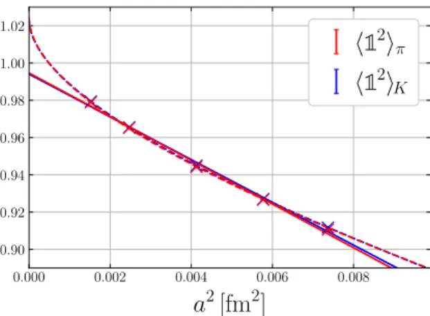
0.000 0.002 0.004 0.006 0.008
a2[fm2]
0.90 0.92 0.94 0.96 0.98 1.00
1.02 12π
12K
Figure 5. The quantity12M as a function of the squared lattice spacinga2, plotted at the physical mass point. The solid lines represent the result of a global fit using eq. (4.1). The points shown have been obtained by translating all data points to the physical masses along the fitted function and then averaging measurements from the same lattice spacing. The dashed curves correspond to the alternative fit carried out to investigate linear terms as described in the main text.
4 Extrapolation strategy and error budget
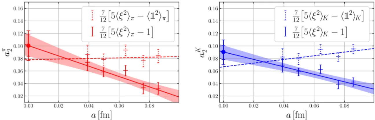
In the following we present our results for the first and the second ξ-moments and Gegen- bauer moments of the leading-twist pseudoscalar meson distribution amplitudes. In addi- tion to the results for the pion and the kaon, which are extracted directly from the lattice data, we infer the second moment of theη8meson using eq. (3.6c) from the SU(3) symmetry breaking constraints obtained from ChPT in ref. [73]. Previous lattice determinations of the Gegenbauer moments [36–43,46,74–78] lacked ensembles with lattice spacings smaller than 0.06 fm and so far no controlled continuum limit extrapolation has been carried out.
This is particularly problematic for the second momentaM2 , which mixes with12M under renormalization, see eqs. (2.16).
4.1 A game of ones
The continuum limit12M a→0
−−−→1 is known. Using this value as a constraint and fitting our data, we find that theadependence is mostly quadratic and the possible linear contribution is small. This is consistent with expectations based on tree-level lattice perturbation theory, where linear terms vanish exactly.
One can play another game, pretend that the continuum value of 12M is not known, and try to determine it from the data. The quadratic fit ansatz
12M =IM +e(2)0,2a2+ ¯e(2)2 m¯2a2+δeM,2(2)δm2a2, (4.1) usingIM as a free parameter, gives a continuum limit value close to one with only 0.5% de- viation, see the solid line in figure 5. This agreement is nontrivial (unrenormalized lattice values in the considered region of lattice spacings lie in the range 0.59–0.68, see, e.g., the left panel of figure4) and can be viewed as confirmation of our calculation of the corresponding renormalization constant.
JHEP08(2019)065
0.05 0.10 0.15
m2π[GeV2]
0.200 0.225 0.250 0.275 0.300 0.325
0.05 0.10 0.15
m2π[GeV2]
0.05 0.10 0.15
m2π[GeV2]
ξ2π
ξ2K
ξ2η8
mu+md+ms= phys. ms= phys. mu=md=ms
Figure 6. Dependence of the momentsξ2M on the squared pion mass, plotted in the continuum limit. The points shown have been obtained by translating all data along the fitted function (keeping the masses fixed). The plots for the individual lattice spacings can be found in figure 12 in appendix A. The solid lines and shaded statistical error bands represent our main result. The dashed curves correspond to the mean value of an alternative fit (including a term of higher order in the masses) used to estimate the parametrization dependence as described in the main text.
However, without the constraint at a= 0, the smallness of linear contributions in com- parison to the quadratic a dependence cannot be inferred from the data: an alternative fit including the additional linear terms e(2)0 a, ¯e(2)m¯2a, and δeM(2)δm2a (dashed curve in figure5) leads to a continuum value that is about 2.5% above unity. The difference can be viewed as a systematic uncertainty of the continuum extrapolation (labeledain the follow- ing), yielding the “lattice values”Iπ = 0.9947+2−2(80)r(301)aandIK = 0.9941+1−2(80)r(300)a, where statistical errors are given by the sub-/superscript pair and the uncertainty due to the renormalization (r) is determined as described in section2.3. To avoid misunderstand- ing: the values of IM (and the fits shown in figure 5) are not used in the determination of the moments of meson LCDAs, to be discussed in the following sections. Their deter- mination merely serves as a sanity check to strengthen the confidence in our renormaliza- tion procedure.
In comparison to our previous work, see figure 3 of ref. [43], we achieve a much higher statistical precision for 12M, such that the statistical error now contributes by far the smallest uncertainty. This improvement in statistics is mostly due to employing the op- eratorO123+ in the new method (2.12b), compared to the old method involving the opera- tors O+4ij, see also the left panel of figure 4. Furthermore, it turns out that also the sys- tematic uncertainties due to renormalization (0.8%) and due to discretization effects (3%) are quite small.
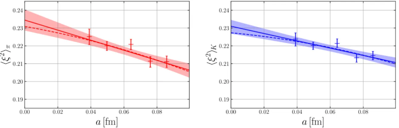
4.2 Extrapolation of the second LCDA moments
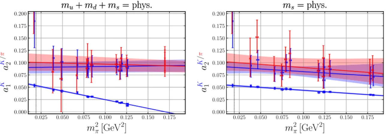
For the extrapolation of the second moments ξ2π and ξ2K we use eq. (3.8b). We then insert the fitted LECs ξ20, ¯A(2), and δA(2) into eq. (3.6c) in order to obtain a prediction forξ2η8 in the continuum. The combined extrapolation is shown in figure 6as a function of the pion mass and in figure 7 as a function of the lattice spacing. Figure6 shows that the breaking of SU(3) flavor symmetry among these observables is rather small. Actually, within our errors, we find no differences betweenξ2π,ξ2K, and ξ2η8. To estimate the
![Figure 1. Models for the pion LCDA: the blue line shows the asymptotic shape corresponding to the limit µ → ∞, while the orange line depicts the CZ model [8, 10] for µ = 0.5 GeV](https://thumb-eu.123doks.com/thumbv2/1library_info/3740279.1509286/4.892.275.620.122.341/figure-models-lcda-shows-asymptotic-corresponding-orange-depicts.webp)