Hadron Distribution Amplitudes from Lattice QCD Simulations

Hadron Distribution Amplitudes from Lattice QCD Simulations

DISSERTATION

ZUR ERLANGUNG DES DOKTORGRADES DER NATURWISSENSCHAFTEN (DR. RER. NAT.)

DER FAKULTÄT FÜR PHYSIK DER UNIVERSITÄT REGENSBURG

vorgelegt von Fabian Hutzler

aus Regensburg

im Jahr 2018

Die Arbeit wurde angeleitet von: Prof. Dr. Andreas Schäfer

Prüfungsausschuss:

Vorsitzender: Prof. Dr. Josef Zweck

1. Gutachter: Prof. Dr. Andreas Schäfer

2. Gutachter: Prof. Dr. Vladimir Braun

weiterer Prüfer: Prof. Dr. Jaroslav Fabian

Abstract

In this thesis we examine hadron distribution amplitudes, which are uni-

versal, process-independent functions that govern the physics of hard ex-

clusive processes and contribute to both, measurements of fundamental

parameters of the Standard Model and probes of new physics. For this

purpose, we perform lattice QCD simulations for mesons and baryons

in order to calculate Mellin moments of the distribution amplitudes nu-

merically.

Contents

1 Introduction 1

2 Quantum chromodynamics on the lattice 5

2.1 Continuum formulation . . . . 5

2.2 Euclidean space-time . . . . 7

2.3 Lattice fermion actions . . . . 8

2.3.1 Naive fermion action . . . . 8

2.3.2 Wilson fermions . . . . 10

2.3.3 Sheikholeslami–Wohlert improvement . . . . 12

2.4 Lattice gauge actions . . . . 14

2.4.1 Wilson gauge action . . . . 14

2.4.2 Lüscher–Weisz gauge action . . . . 15

2.5 Correlation functions and path integrals . . . . 16

2.5.1 Correlators . . . . 16

2.5.2 Grassmann integrals . . . . 17

3 Simulation methods 19 3.1 General idea . . . . 19

3.2 Hybrid Monte Carlo . . . . 21

3.2.1 Inclusion of the light sea quarks . . . . 22

3.2.2 Inclusion of the strange sea quarks . . . . 22

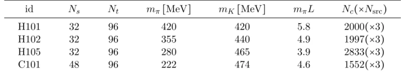
3.3 Ensembles . . . . 23

3.3.1 Open boundary conditions . . . . 23

3.3.2 Twisted mass reweighting and preconditioning . . . . 24

3.3.3 CLS ensembles . . . . 25

3.3.4 Other ensembles . . . . 27

4 Baryon distribution amplitudes 29 4.1 Overview . . . . 29

4.2 Continuum formulation . . . . 32

4.2.1 Leading twist distribution amplitudes . . . . 33

4.2.2 Higher twist contributions . . . . 37

4.3 Lattice formulation . . . . 38

4.3.1 Correlation functions . . . . 39

4.3.2 Details and strategy of the lattice simulation . . . . 43

4.4 Data analysis . . . . 44

4.5 Results . . . . 50

4.6 Summary and outlook . . . . 56

5 Meson distribution amplitudes 57 5.1 Pion distribution amplitude . . . . 57

5.1.1 Overview . . . . 57

5.1.2 Continuum formulation . . . . 59

5.1.3 Lattice formulation . . . . 60

5.1.4 Simulation details and momentum smearing . . . . 62

5.1.5 Optimizing the smearing and the momentum . . . . 65

5.1.6 Momentum smearing versus Wuppertal smearing . . . . 66

5.1.7 Chiral extrapolation . . . . 68

5.1.8 Summary and outlook . . . . 70

5.2 Rho-meson distribution amplitudes . . . . 71

5.2.1 Overview . . . . 71

5.2.2 Continuum formulation . . . . 71

5.2.3 Lattice formulation . . . . 73

5.2.4 Lattice correlation functions . . . . 74

5.2.5 Decay constants . . . . 75

5.2.6 Second moments . . . . 76

5.2.7 Details of the lattice simulations . . . . 78

5.2.8 Data analysis . . . . 79

5.2.9 Results and conclusion . . . . 83

6 Conclusion and outlook 87

7 Bibliography 91

1 Introduction

In the mind of contemporary physicists, the development of quantum chromodynamics (QCD), the theory of the strong interaction, marked a radical change of perception of our physical world: During the 1950s, it was common belief that all hadrons like the proton or pion are equally elementary particles as reflected by the concept of nuclear democracy or hadronic egalitarianism [1–4]. However, this view had changed completely by the end of the 70s and it has since been generally accepted that hadrons are composed of fractionally charged fermionic quarks that are bound together by electrically neutral gluons, the gauge bosons of the theory which act as mediators of the strong force between the quarks.

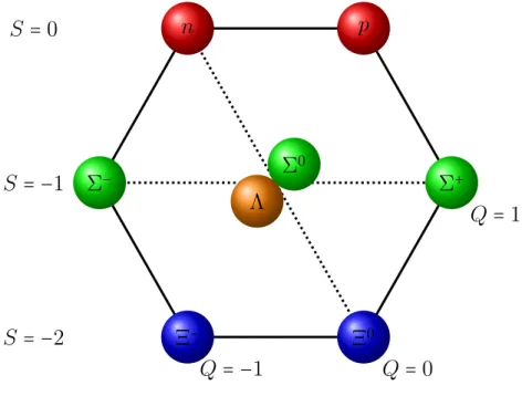
In order to satisfy the spin-statistics theorem [5] for ground state hadron multiplets, refs. [6–8] proposed the existence of an additional quantum number that is nowadays known as color. Consequently, each quark was assigned one of the three color charges red , blue or green . In fact, QCD is a Yang-Mills theory [9] with the underlying non-abelian gauge group SU ( 3 )

. Therefore, each quark is represented by a triplet of fields, while the gluons form a color octet. Quarks and gluons exhibit color confinement, which means that below the Hagedorn temperature they cannot be observed as free particles and are therefore bound in color-singlet hadronic states. The reason for this is that the QCD one-loop beta function is negative for N

≤ 16, which is a consequence of the non-abelian nature of the theory that allows self-interacting gauge bosons. As a result, the quark interaction becomes weaker for higher momentum transfers Q

, such that quarks behave asymptotically free at large energies. In contrast, the strong coupling constant grows for smaller Q

, which leads to the confinement of quarks within hadrons. Hadrons themselves can be further classified into two subgroups, namely baryons and mesons. The former are composite fermions which contain three valence quarks while the latter are bosons with a quark-antiquark pair valence structure. The Standard Model involves quarks of six different flavors: up- , down- , charm- , strange- , top- and bottom- quarks. Their masses range over several orders of magnitude, from the light up-quark with m

= 2.2 MeV to the heavy top quark which has almost the mass of a gold atom with m

= 173.1 GeV [10].

Due to the intrinsically non-perturbative nature of confinement, hadron structure in

terms of quarks and gluons is highly non-trivial. It can be described with universal

process-independent QCD functions like parton distribution functions (PDFs) and hadron

distribution amplitudes (DAs), which are relevant for both, measurements of fundamental

parameters of the Standard Model and probes of new physics. PDFs are needed to describe

deep inelastic scattering (DIS) experiments [11–16], where the inner structure of hadrons is resolved by probing them inclusively with leptons. In order to understand the inelastic scattering process, it is helpful to consider the naive parton model [17], where the hadronic structure functions that parametrize the differential cross section become independent of the momentum transfer Q

in the asymptotic limit [18]. This so-called Bjorken scaling behavior can be understood in the infinite-momentum frame, where the hadron is consid- ered as a ray of collinear quasi-free partons. Consequently, at a large enough momentum transfer Q

, the incoming lepton directly scatters with a quasi-free quark that carries the longitudinal momentum fraction x of the hadron, such that the resulting process can be described as lepton-quark scattering instead of lepton-hadron scattering. Early measure- ments showed that quarks are merely responsible for half of the nucleon’s momentum [19], so that the remaining momentum has to be carried by electromagnetically non-interacting partons that were eventually identified as gluons. Strictly speaking, the naive parton model is an approximation of QCD which is only valid for vanishing coupling strength. In reality, Bjorken scaling is somewhat violated. As a consequence, PDFs exhibit a scale de- pendence which is governed by the famous DGLAP equations [20–22]. Thus, at a certain energy scale Q

, a PDF specifies the probability density to find a parton of a certain kind that carries the longitudinal momentum fraction x of the hadron.

In this work, however, we will focus on hadron distribution amplitudes, which are fun-

damental non-perturbative functions that can be interpreted as light-cone wave functions

integrated over transverse quark momenta [23, 24]. Because of this, they are sensitive to

those Fock states of the hadronic wave function which govern exclusive processes with

large momentum transfer Q

. In the limit Q

→ ∞ , distribution amplitudes are given

by their so-called asymptotic expressions [23–25], which, however, deviate significantly

from their form at experimentally accessible momentum transfers. Therefore, in view of

constantly increasing luminosities of modern research facilities like the 12 GeV upgrade

at JLAB [26] or the future EIC [27], a precise determination of hadron distribution am-

plitudes is essential in order to provide rigorous theoretical descriptions of hard exclusive

processes. Compared to PDFs, the connection between DAs and experimentally accessible

observables is more challenging. Especially the relations between hadronic form factors

and hadron distribution amplitudes are of particular importance. For example, it is known

that for very high momentum transfers Q

, hard exclusive processes like elastic electron-

nucleon scattering are dominated by hard gluon exchange contributions [23, 25, 28], such

that the baryonic form factor is given by a convolution of two distribution amplitudes

with a hard scattering kernel. In this case, the same logic applies as for inclusive DIS

processes, i.e., the interaction between the electron and the nucleon can be pictured as

electron-quark scattering in the infinite-momentum frame. As the hit quark has obtained

a large transverse momentum it must exchange gluons with the remaining quarks in order

to merge into an outgoing baryon again. The fact that all incoming and outgoing quarks within the elastic process are confined in color-singlet states cancels potential soft interac- tions between the initial and final quarks in the scattering kernel and enables a Fock state expansion of the involved hadronic wave functions [23]. On the light-cone, the leading term of this expansion is given by the valence Fock state, i.e., the Fock state with the minimal number of constituent quarks for the respective hadron. As each gluonic exchange involves an additional factor of α

/ Q

in the hard scattering kernel, higher non-valence Fock states can be neglected. In this picture, the probability amplitude to observe a many-parton state confined into a small transverse volume is suppressed [29]. As a result, the informa- tion content obtained from distribution amplitudes is complementary to that of parton distribution functions: While a PDF always describes the hadron as a whole and does not discriminate between Fock states, a distribution amplitude corresponds to the probability amplitude to find the partons with a certain momentum distribution within a single Fock state. At experimentally achievable intermediate values of Q

, the small prefactors of the perturbative calculation cause soft contributions to dominate the behavior of hadronic form factors. In order to account for this, light-cone sum rules (LCSR) have successfully been applied to both meson [30] and baryon [31] form factors at intermediate momentum transfers.

The main goal of this thesis is the determination of hadron distribution amplitudes using lattice QCD simulations. The advent of lattice QCD can be dated to 1974 when Wilson published the first formulation of gauge theories on a discretized space-time lattice [32].

This new approach, however, did not fully establish itself until 1979, when Creutz et

al. [33] and Wilson [34] showed how to calculate hadronic observables by purely statistical

computer simulations. This was immediately followed by successful attempts to calculate

the SU ( 2 ) static quark-antiquark potential [35] as well as various hadron masses [36,37] on

the lattice. Nowadays, lattice QCD is accepted as the tool to investigate non-perturbative

phenomena and provides high-precision results due to a combination of sophisticated algo-

rithms [38] and ever growing processing power. The first attempts to calculate distribution

amplitudes on a lattice were conducted for the second moment ⟨ ξ

⟩ of the pion DA more

than 30 years ago [39,40]. In the meantime, lattice results have been obtained for various

hadrons, including the pion, the kaon, the rho and the nucleon [41–44]. In this work, we

will present results of multiple recent lattice studies, including the first calculation of the

DAs of the baryon octet, a calculation of the second moments of the rho meson as well

as a calculation of the pion DA using a new smearing technique. The outline of this work

is structured as follows: The 2nd chapter introduces both, QCD in the continuum as well

as QCD on the lattice. The 3rd chapter explains the utilised simulation methods with a

focus on the lattice ensembles of the CLS effort. Chapter 4 is dedicated to baryon distri-

bution amplitudes and presents a N

= 2 + 1 calculation of the zeroth and first moments

of the DAs of the baryon octet. Chapter 5 is devoted to meson distribution amplitudes and is divided into two parts: Section 5.1 introduces a new smearing technique for the second moments of the distribution amplitude of the pseudoscalar pion. Subsequently, the results of a recent N

= 2 study of the DAs of the ρ-meson are presented in section 5.2.

Chapter 6 concludes this thesis by giving a short summary as well as an outlook for future

developments.

2 Quantum chromodynamics on the lattice

2.1 Continuum formulation

This section is dedicated to the fundamentals of QCD in the continuum and focuses on the derivation of the classical QCD Lagrangian as a starting point for the lattice discretization in section 2.3. Since we only consider gauge-invariant observables on the lattice, we do not discuss the Faddeev-Popov method [45] and the BRST quantization [46–49] but refer the interested reader to the textbooks [50,51].

QCD is a non-abelian gauge field theory with the special unitary group SU ( 3 )

as its underlying gauge group. Hence the 3

− 1 independent generators give rise to 8 massless spin 1 gauge bosons, the gluon fields A

( a = 1, . . . , 8 ) . The QCD Lagrangian L

can be constructed by applying the gauge principle with respect to the color group SU ( 3 )

to the Lagrangian L

of a free fermionic spin 1 / 2 quark field ψ of single flavor:

L

= ∑

i,i^′

∑

αα^′

ψ ¯

( i ∂ /

− mδ

δ

) ψ

, (2.1)

with ∂ / = ∂

γ

, ¯ ψ = ψ

γ

, the Dirac-spinor index α = 1, . . . , 4 and color i = 1, 2, 3. Due to the partial derivatives, eq. (2.1) is not invariant under the local gauge transformation

ψ ( x ) → ψ

( x ) = Ω ( x ) ψ ( x ) , (2.2) where Ω ( x ) = e

∈ SU ( 3 )

. In the fundamental representation, the generators t

of SU ( 3 ) can be expressed as t

=

, where the λ

are the traceless Hermitian Gell-Mann matrices as introduced in ref. [52]. We replace the partial derivatives in eq. (2.1) by the covariant derivatives

D

= ∂

+ iA

t

≡ ∂

+ iA

, (2.3) where A

≡ A

t

. As a result, the fermionic Lagrangian,

L

= ∑

i,i^′

∑

αα^′

ψ ¯

( i D /

− mδ

δ

) ψ

, (2.4)

is now gauge invariant if the gauge potential A

transforms as

A

→ A

= ΩA

Ω

+ i ( ∂

Ω ) Ω

. (2.5) In order to describe the dynamics of the gluon fields, the final Lagrangian must also contain a kinetic term which is only composed of the gauge fields A

. For this purpose, similar to QED, one defines the non-abelian field strength tensor

F

= ∂

A

− ∂

A

+ i [ A

, A

] = − i [ D

, D

] . (2.6) Using that Tr ( λ

λ

) = 2δ

, one obtains the gluon Lagrangian as

L

= − 1

4g

F

F

= − 1

2g

Tr ( F

F

) , (2.7) where g is the gauge coupling and again F

= F

t

. As already mentioned in the introduction, the Standard Model involves six quark flavors, ( f = u, d, s, c, b, t ) , such that we now can obtain the final QCD Lagrangian, which is by construction invariant under local SU ( 3 )

gauge transformations:

L

= L

+ L

= ∑

f

∑

i,i^′

∑

α,α^′

ψ ¯

( i D /

− m

δ

δ

) ψ

− 1

2g

Tr ( F

F

)

= ∑

f

ψ ¯

( x )( i D / − m

) ψ

( x ) − 1

2g

Tr ( F

F

) . (2.8) The QCD vacuum is highly non-trivial and contains infinitely many vacuum states [53], such that, in general, eq. (2.8) has to be complemented by another gauge-invariant term which governs the vacuum topology. This so-called θ-term is of the form

L

= θ

64π

F

F

= θ

32π

F

F ˜

. (2.9)

Here θ is real and ˜ F

=

F

is the dual field strength tensor. As

is a

pseudotensor, this term acquires a minus sign under parity transformations and thus

would violate P and CP symmetry. Experimentally, the θ-term can best be probed by

measurements of the neutron electric dipole moment (nEDM). To satisfy experimental

bounds on the nEDM [54–58], the θ-parameter has to be very small, θ ≤ 10

, and

will be neglected in the following. The unexplained smallness of θ poses a fine-tuning

problem that leads to the famous strong CP problem. A proposed solution is given by the

Peccei-Quinn mechanism [59], which introduces pseudoscalar axions as a consequence of

the spontaneously broken U ( 1 ) Peccei-Quinn symmetry.

2.2 Euclidean space-time

2.2 Euclidean space-time

Since the indefinite metric of QCD in Minkowski space gives rise to n-point correlation functions that oscillate in time, lattice calculations are carried out in Euclidean space- time. This is achieved by a so-called Wick rotation, an analytical continuation of the time component to imaginary values,

t → it , (2.10)

which was first applied by Dyson to avoid poles in contour integrals in QED [60]. The Minkowski and Euclidean space-time coordinates are then connected in the following way:

x

= x

= − x

, (2.11a)

x

= ix

= ix

. (2.11b)

For example, this means with respect to the gluon Lagrangian that L

= − 1

2g

Tr( F

F

) = − 1

2g

Tr( F

F

) = −L

, (2.12) such that the action functional gives

S

= ∫ d

x L

= ∫ dx

∫ d

x L

= i ∫ dx

∫ d

x

L

= iS

, (2.13) and this “Wick rotation” effectively yields

e

→ e

. (2.14)

It is possible to recover the Hilbert space quantum field theory from a Euclidean field theory if certain conditions, such as reflection positivity, are fulfilled [61], guaranteeing the Wick rotation to be a well-defined isomorphism between Minkowski and Euclidean space-time theories. The Wick rotation connects the Euclidean field theory to classical statistical mechanics. The direct equivalence between both theories can be illustrated by considering the similarities between the Boltzmann weight factor and the Feynman weight for amplitudes:

e

⇐⇒ e

. (2.15)

Recognizing the impact of eq. (2.15) is crucial for the understanding of lattice QCD, as

this equivalence allows us to attack problems of the field theory with already established

methods of statistical mechanics. As an illustrative example, the calculation of the vacuum

expectation value ⟨ 0 ∣O∣ 0 ⟩ of an observable O on the lattice corresponds to the calculation of the canonical ensemble average ⟨ O ⟩ of an observable O in classical statistical mechanics.

2.3 Lattice fermion actions

An introduction to lattice QCD can be found in many textbooks on lattice gauge theories or quantum field theories. In the next sections we follow the introductory presentations of refs. [62–64].

We begin by considering the four-dimensional lattice ` of size N

N

, which contains N

points in each spatial direction and N

points in the time direction. The vectors n

form the grid points of the lattice, which are separated by the dimensional lattice spacing a from their neighbours and fulfill

` = { n ∈ ( n

, n

, n

, n

) ∣ n

, n

, n

= 0, . . . , N

− 1; n

= 0, . . . , N

− 1 } , (2.16) such that physical space-time coordinates are recovered by x

= an

. In particular we will often refer to the lattice time t = an

, the spatial extent L = aN

and the time extent T = aN

in the following.

2.3.1 Naive fermion action

Having defined the raw lattice `, our goal is now to construct a discretized lattice version of the Euclidean fermionic action that approaches the Euclidean continuum version

S

= ∫ d

x ψ ( x )( γ

( ∂

+ iA

( x )) + m ) ψ ( x ) , (2.17) in the limit a → 0. In order to achieve this, we proceed in a similar constructive manner as for the derivation of the QCD Lagrangian in section 2.1. On the lattice, the continuous integral over the four-dimensional space-time of eq. (2.17) becomes a sum over all points of ` such that

∫ d

x → a

∑

x

. (2.18)

Furthermore, we symmetrically discretize the partial derivative that acts on the fermionic fields to get

∂

ψ ( x ) = ψ ( x + aˆ µ ) − ψ ( x − aˆ µ )

2a , (2.19)

2.3 Lattice fermion actions where ˆ µ denotes the unit vector in the µ direction. In this way, we obtain an expression for the free lattice action, similar to the free continuum Lagrangian in eq. (2.1):

S

= a

∑

x

ψ ( x )( ∑

µ=1

γ

ψ ( x + aˆ µ ) − ψ ( x − aˆ µ )

2a + mψ ( x )) . (2.20)

As in the continuum case, due to the partial derivatives, this expression is not invariant under local gauge rotations defined in eq. (2.2), since

ψ

( x ) ψ

( x + aˆ µ ) = ψ ( x ) Ω

( x ) Ω ( x + aˆ µ ) ψ ( x + aˆ µ ) . (2.21) In the continuum, gauge invariance is restored in eq. (2.3) by replacing the partial deriva- tives with covariant derivatives which contain the gluon fields A

. On the lattice, the covariant derivatives are achieved by introducing the fields U

( x ) , which transform as

U

( x ) = Ω ( x ) U

( x ) Ω

( x + aˆ µ ) , (2.22) such that

ψ

( x ) U

( x ) ψ

( x + a µ ˆ ) = ψ ( x ) Ω

( x ) U

( x ) Ω ( x + a µ ˆ ) ψ ( x + a µ ˆ ) (2.23) becomes gauge invariant. As an element of SU ( 3 ) , the gauge field U

( x ) connects the two neighbouring grid points x and x + aˆ µ, which gives rise to its name as gauge link . The gauge link U

( x + aˆ µ ) , which connects the point x + aˆ µ with x, and its oppositely orientated counterpart U

( x ) , which connects the point x with x + aˆ µ, are related by

U

( x + aˆ µ ) = U

( x ) . (2.24) We now introduce the lattice gauge fields A

( x ) by defining

U

( x ) = exp ( iaA

( x )) . (2.25) Finally, for interacting fermions on the lattice we obtain the so-called naive fermion action :

S

= a

∑

x

ψ ( x )( ∑

µ=1

γ

U

( x ) ψ ( x + aˆ µ ) − U

( x ) ψ ( x − aˆ µ )

2a + mψ ( x )) . (2.26)

By using matrix-vector notation, we can rewrite eq. (2.26) to obtain the familiar expression S

= a

∑

x,y α,β,i,j

ψ

( x ) D

( x, y ) ψ

( y ) , (2.27)

with the Dirac operator

D

( x, y ) = ∑

µ

( γ

)

U

( x ) δ

− U

( x ) δ

2a + mδ

δ

δ

. (2.28) In order to check the proper continuum behavior of eq. (2.26), we consider the limit of small lattice spacing a, where

U

( x ) = 1 + iaA

( x ) + O( a

) , (2.29) and neglect the O( a

) terms to obtain

S

= a

∑

x

ψ ( x )( ∑

µ=1

γ

ψ ( x + aˆ µ ) − ψ ( x − aˆ µ )

2a + mψ ( x ))

+ ia

∑

x

∑

µ=1

ψ ( x ) γ

1

2 ( A

( x ) ψ ( x + aˆ µ ) + A

( x − aˆ µ ) ψ ( x − aˆ µ ))

= S

+ ia

(∑

x

∑

µ=1

ψ ( x ) γ

A

( x ) ψ ( x ) + O( a )) . (2.30) Hence, we recover the continuum action of eq. (2.17) in the limit a → 0 with discretization errors of O( a ) .

2.3.2 Wilson fermions

By further investigating the lattice Dirac operator we find that the naive action in eq. (2.26) actually yields 16 Dirac particles instead of one. We start by comparing the lattice quark propagator with its continuum counterpart

S ( p ) = m − iγ

p

m

+ p

. (2.31)

For this, we calculate the Fourier transformation of the naive Dirac operator in eq. (2.28) for the free case and obtain

D ˜ ( p, q ) = δ ( p − q ) D ˜ ( p ) , (2.32) with

D ˜ ( p ) = m1 + i a ∑

µ

γ

sin ( p

a ) . (2.33)

2.3 Lattice fermion actions

For massless fermions, the momentum-space propagator ˜ D

( p ) is then given by D ˜

( p ) = −

∑

γ

sin ( p

a )

1

a²

∑

sin ( p

a )

. (2.34) At first sight, this result seems reassuring as we recover eq. (2.31) for m = 0 in the continuum limit

D ˜

( p )

→ − iγ

p

p

= S ( p )∣

m=0

. (2.35)

However, due to the periodicity of the sine function, eq. (2.34) exhibits a pole whenever each component of p

is either 0 or

, which leaves us with 2

= 16 combinations. Beside the natural pole at p

= 0, the 15 additional poles are referred to as doublers . In order to get rid of these additional poles, Wilson suggested to modify the fermion action by adding the momentum-dependent term

mψψ → mψψ + a

2 ∂

ψ∂

ψ , (2.36)

to the mass term [63]. Thus the Dirac operator in momentum space gives D ˜ ( p ) = m1 + 1

a ∑

µ

1 ( 1 − cos ( p

a )) + i a ∑

µ

γ

sin ( p

a ) . (2.37) The so-called Wilson term does not give any contribution for the natural pole at p

= 0, while it acts as an additional mass term for poles with momentum components p

=

, such that

m

→ m

+ N

2

a , (2.38)

where N

is the number of momentum components that are equal to

. In this way the mass of the unintended doublers is increased to the order of the cutoff, which decouples them from physics in the continuum. After incorporating eq. (2.36), the lattice Dirac operator of a fermion f in the interacting case can simply be written as

D

αβ

( x, y ) = − 1 2a ∑

±µ

( 1 − γ

)

αβ

U

( x ) δ

+ ( m

+ 4

a ) δ

δ

δ

, (2.39) where for convenience we introduced the compact notation

∑

= ∑

µ=±1

, (2.40a)

γ

= − γ

. (2.40b)

An important symmetry of the Wilson Dirac operator is the so-called γ

-Hermiticity

D

= γ

Dγ

, (2.41)

which also holds for its inverse such that

D

= γ

D

γ

. (2.42)

Eq. (2.41) also means that the eigenvalues of the Wilson Dirac operator are either real or complex conjugate pairs as

det ( D − λ1 ) = det ( D

− λ1 ) = det ( D − λ

1 )

. (2.43) Finally, the Wilson fermion action for multiple flavors is given by

S

= ∑

f

a

∑

x,y α,β,i,j

ψ

( x ) D

( x, y ) ψ

( y ) . (2.44)

2.3.3 Sheikholeslami–Wohlert improvement

The fermion lattice action in eq. (2.44) suffers from discretization errors of O( a ) which distort the lattice results and subsequent continuum extrapolations. In this section we therefore derive the counterterms to the lattice action which are required for an on-shell O( a ) improvement. Following [65,66], we describe the lattice theory for finite a as a local effective theory which recovers the continuum action S

in the limit a → 0 such that

S

= S

+ aS

+ a

S

+ . . . , (2.45) where

S

= ∫ d

x L

( x ) . (2.46)

The so-called correction terms L

( x ) are of dimension 4 + k and contain additional powers of the mass or additional derivatives. For an O( a ) improvement we want to identify and cancel the L

contribution and thus consider only fields with an energy dimension of 5.

In addition, the resulting terms should be gauge invariant and respect the space-time

and charge conjugation symmetries of the lattice. It turns out that L

must be a linear

2.3 Lattice fermion actions

combination of the following 5 fields:

O

= ψσ

F

ψ , (2.47a)

O

= ψ D ⃗

D ⃗

ψ + ψ D ⃗

D ⃗

ψ , (2.47b)

O

= m Tr ( F

F

) , (2.47c)

O

= mψγ

D ⃗

ψ − mψ D ⃗

γ

ψ , (2.47d)

O

= m

ψψ . (2.47e)

Using the field equations of the continuum theory allows us to eliminate eq. (2.47b) and eq. (2.47d), which further reduces the number of possible fields. We now want to improve our fermion action by adding a counterterm δS to the Wilson action such that L

is eliminated and thus the O( a) discretization effects are canceled. The counterterm δS can only be composed of the 3 remaining fields:

δS

= a

∑

x

( c

O

( x ) + c

O

( x ) + c

O

( x )) , (2.48) where O

is the lattice version of the respective field in eqs. (2.47). The structures Tr ( F

F

) and ψψ already appear in the Wilson gauge and Wilson fermion action and can be accounted for by a renormalization of the bare coupling and mass. Therefore it is only necessary to add one term with the structure of eq. (2.47a) and we obtain the counterterm

δS

[ U, ψ, ψ ] = a

∑

x

c

ψ ( x ) 1

2 σ

F

( x ) ψ ( x ) , (2.49) where c

is the so-called Sheikholeslami–Wohlert coefficient , which is real and can be calculated numerically, cf. [67]. The lattice version of the Euclidean field strength tensor can be written as

F

( x ) = − i

8a

( Q

( x ) − Q

( x )) , (2.50) with the sum over all adjacent plaquettes

Q

( x ) = U

( x ) + U

( x ) + U

( x ) + U

( x ) . (2.51)

Due to its four-fold symmetry in a two-dimensional plane, eq. (2.49) is referred to as clover

term .

2.4 Lattice gauge actions

2.4.1 Wilson gauge action

The construction of the gluon lattice action is governed by three guidelines: The action has to be gauge invariant, it can only consist of gauge fields and it has to yield the continuum gauge action

S

= 1

2g

∫ d

x Tr ( F

( x ) F

( x )) , (2.52) in the limit a → 0. Equivalent definitions in terms of the inverse squared coupling β =

are also found in the literature. We first consider the smallest closed loop U

( x ) on the lattice:

U

( x ) = U

( x ) U

( x + aˆ µ ) U

( x + aˆ ν ) U

( x ) . (2.53) U

( x ) can be illustrated as a square along the four gauge links and thus is referred to as plaquette in the literature. The trace of every closed loop of gauge links is gauge invariant due to the cyclic properties of the trace. Therefore we define the so-called Wilson gauge action [32] as a sum over all possible plaquettes:

S

[ U ] = 2 g

∑

x

∑

µ<ν

Re Tr ( 1 − U

( x )) . (2.54) The behavior in the continuum limit can be checked by applying the Baker-Campbell- Hausdorff formula

exp ( A ) exp ( B ) = exp ( A + B + 1

2 [ A, B ] + . . . ) , (2.55) together with the Taylor expansion

A

( x + aˆ µ ) = A

( x ) + a∂

A

( x ) + O( a

) . (2.56) As a result, we get:

U

( x ) = exp ( ia

( ∂

A

( x ) − ∂

A

( x ) + i [ A

( x ) , A

( x )]) + O( a

))

= exp ( ia

F

( x ) + O( a

)) . (2.57) We insert this expression for U

into eq. (2.54) and obtain

S

[ U ] = a

2 g

∑

x∈`

∑

µ,ν

Tr ( F

F

) + O( a

) , (2.58)

2.4 Lattice gauge actions

S

S

S

S

Figure 2.1: Elementary loops contained in each set S

. which yields eq. (2.52) for a → 0.

2.4.2 Lüscher–Weisz gauge action

Similar to the Sheikholeslami–Wohlert improvement for the fermion action, the Wilson gauge action can be improved by adding a linear combination of 3 operators of dimension 6 to the standard plaquette. We follow [68] and make the ansatz

S

[ U ] = 2 g

∑

i=0

c

( g

) ∑

C∈Si

Re Tr [ 1 − U (C)] , (2.59) where the S

denote the sets of elementary loops C of a certain kind, while U (C) is the oriented product of link variables U

( x ) along C . Figure 2.1 shows a sketch of the possible elementary loops C that appear in eq. (2.59). In compliance with eq. (2.54), S

is the set of oriented 1 × 1 plaquettes, while S

contains all 1 × 2 rectangular loops. S

and S

are more complicated and extend in 3 dimensions, cf. figure 2.1. In order to achieve a tree-level improved action, Lüscher and Weisz showed that one coefficient can be chosen freely [69], such that to lowest order in g

, the most general on-shell improved action is given by

c

( 0 ) = 5

3 − 24x , (2.60a)

c

( 0 ) = − 1

12 + x , (2.60b)

c

( 0 ) = 0 , (2.60c)

c

( 0 ) = x . (2.60d)

For the reader’s convenience we will suppress the superscript lat. in the following and

always use the lattice action unless stated explicitly otherwise.

2.5 Correlation functions and path integrals

2.5.1 Correlators

Having constructed the appropriate QCD action on the lattice, we will now establish a connection between the observables of interest and the numerically evaluable path integral on the lattice. To this end we define the Euclidean correlator of two operators ˆ O

and ˆ O

as

⟨ O

( t ) O

( 0 )⟩ = 1

Z Tr [ e

O ˆ

e

O ˆ

] , (2.61) with the Hamiltonian of the system ˆ H and the partition function Z = Tr [ e

] . The field operators appearing in eq. (2.61) can measure observables or create and annihilate particles with certain quantum numbers. We will denote ˆ O

as the operator that creates a state with the quantum numbers of the hadron H, while its adjoint partner ˆ O

annihilates this state or creates a state with the quantum numbers of its antiparticle H. Using the eigenvalue equation

H ˆ ∣ n ⟩ = E

∣ n ⟩ , (2.62)

we expand eq. (2.61) by inserting a complete set of states. After normalizing the vacuum energy E

to zero we obtain the limit

T

lim

⟨ O

( t ) O

( 0 )⟩ = ∑

n

⟨ 0 ∣ O ˆ

∣ n ⟩⟨ n ∣ O ˆ

∣ 0 ⟩ e

. (2.63) Let H be a hadron with the corresponding annihilation and creation operators O

and O

, respectively. For this case eq. (2.63) yields

T

lim

⟨ O

( t ) O

( 0 )⟩ = ∣⟨ H ∣ O ˆ

∣ 0 ⟩∣

e

+ ∣⟨ H

∣ O ˆ

∣ 0 ⟩∣

e

+ . . . , (2.64) where ∣ H ⟩ denotes the ground state of the hadron H, while ∣ H

⟩ , ∣ H

⟩ , . . . denote excited states with the quantum numbers of H. All states which possess these quantum num- bers contribute to the correlator with a coefficient that falls off exponentially with the respective energy of the state. All other contributions from states that do not possess the quantum numbers of the hadron H vanish. For high lattice times t, the excited states have sufficiently decayed and only the ground state contributes, which allows us to analyse its energy and matrix element.

In order to calculate the Euclidean correlator on the lattice, we employ the Feynman

2.5 Correlation functions and path integrals

path integral formalism such that

⟨ O

( t ) O

( 0 )⟩ = 1

Z ∫ D[ ψ, ψ ]D[ U ] e

O

[ ψ, ψ, U ] O

[ ψ, ψ, U ] , (2.65) with the partition function

Z = ∫ D[ ψ, ψ ]D[ U ] e

. (2.66) The integral in eq. (2.65) runs over all values of the quark fields ψ and ¯ ψ, as well as over the gluon fields U at every space-time point. The corresponding integral measures are products of measures of all quark fields and all gauge links

D[ ψ, ψ ] = ∏

x

∏

f,α,i

dψ

( x ) d ψ ¯

( x ) , (2.67a) D[ U ] = ∏

x

∏

µ=1

dU

( x ) , (2.67b)

where dU denotes the normalized Haar measure on SU ( 3 ) [63,70].

2.5.2 Grassmann integrals

Due to Pauli’s exclusion principle, the integration of the fermionic fields ψ and ψ is inher- ently different from the integration of the gauge links U . Let O be a generic product of operators

O = ∏

n=1

ψ

( x

) ψ

( y

) , (2.68) we then rewrite eq. (2.65) such that

⟨ O ⟩ = 1

Z ∫ D[ U ] e

Z

[ U ]⟨ O ⟩

[ U ] , (2.69) with the fermionic part of the correlator

⟨ O ⟩

[ U ] = 1

Z

[ U ] ∫ D[ ψ, ψ ] e

O [ ψ, ψ, U ] , (2.70) and the fermionic partition function

Z

[ U ] = ∫ D[ ψ, ψ ] e

. (2.71)

In this way we separate the fermionic and bosonic integrals in order to account for their different nature. The fermionic fields ψ and ψ have to obey Fermi statistics, which means that ⟨ O ⟩ has to acquire a minus sign if the quantum numbers of two fermions are inter- changed. We implement this correct anti-commutation behavior by introducing ψ and ψ as Grassmann numbers with the properties

{ ψ

( x ) , ψ

( y )} = 0 , (2.72a)

∂

∂ψ

( y ) ψ

( x ) = ∫ dψ

( y ) ψ

( x ) = δ

δ

δ

. (2.72b) Realizing these Grassmann numbers in a computer simulation would be tedious but in practice this is not required anyway as the fermionic fields can be integrated out before the simulation. Using the properties (2.72), the fermionic partition function can be expressed as the determinant of the Dirac operator:

Z

[ U ] = ∫ D[ ψ, ψ ] exp (− a

∑

x,y α,β,i,j

ψ

( x ) D

( x, y ) ψ

( y ))

= det (− a

D ) . (2.73)

We use the translational invariance of Grassmannian integration and generalize eq. (2.73) by making the translations ψ → ψ − a

θD

and ψ → ψ − a

D

θ to obtain

∫ D[ ψ, ψ ] exp (− a

∑

x,y α,β,i,j

ψ

( x ) D

( x, y ) ψ

( y ) + ∑

α,ix

θ

( x ) ψ

( x ) + ∑

α,ix

ψ

( x ) θ

( x ))

= det (− a

D ) exp ( a

∑

x,y α,β,i,j

θ

( x )( D

)

( x, y ) θ

( y )) , (2.74) which we will use as a generating functional for fermions. The inverse of the lattice Dirac operator D

is referred to as quark propagator . By applying derivatives with respect to θ and θ in eq. (2.74) we obtain the so-called Wick theorem:

⟨ ∏

n=1

ψ

( x

) ψ

( y

)⟩

= 1

Z

∫ D[ ψ, ψ ]( ∏

n=1

ψ

( x

) ψ

( y

)) exp (− a

∑

x,y α,β,i,j

ψ

( x ) D

( x, y ) ψ

( y ))

= ∑

π∈SN

sgn ( π ) ∏

n=1

( a

D

)

( x

, y

) . (2.75)

The Wick theorem allows us to reduce products of quark field operators to sums of products

of quark propagators, which can be calculated on the lattice, cf. eq. (2.69).

3 Simulation methods

3.1 General idea

In the following we will describe the simulation details and techniques which were used for the lattices analysed in this work. In particular, we will focus on the N

= 2 + 1 ensembles generated by the Coordinated Lattice Simulations (CLS) community effort.

Having integrated out the fermionic degrees of freedom in section 2.5.2, we are merely left with an integration over the gauge links U. Employing N

= 2 + 1 dynamical fermions, the corresponding path integral has the form

⟨ O ⟩ = 1

Z ∫ D[ U ] e

det ( D

) det ( D

) det ( D

) ⟨ O ⟩

. (3.1) Eq. (3.1) is a high-dimensional group integral for each link of the whole lattice and already extremely expensive to calculate for very small lattice sizes. As an illustrative example, we consider a four-dimensional lattice of the size 10 × 10 × 10 × 10 which contains 4 · 10

gauge links. Each of the SU ( 3 ) gauge links contains 8 real parameters, which results in 320000 integrations. Approximating the integral by a mesh of 10 points per integration already yields a sum of 10

terms [64], which obviously cannot be computed in practice.

Therefore, sophisticated numerical methods are needed for the evaluation. Fortunately, due to the direct equivalence between Euclidean field theories and classical statistical mechanics as shown in eq. (2.15), we can use well-established techniques that were initially developed for statistical mechanics systems. In particular we will employ the Metropolis Monte Carlo algorithm, which was introduced in 1953 [71] to numerically handle multi- dimensional integrals for interacting individual molecules and spin systems. Following [72]

we introduce the Monte Carlo method for a generic statistical mechanics system. Let H be the Hamiltonian of the system which is characterized by the set of variables x , while f is the observable of interest. The expectation value of f is given by

⟨ f ⟩ = ∑

f ( x ) e

∑

e

. (3.2)

Using the Monte Carlo method, we approximate ⟨ f ⟩ by the evaluation of the sequence

f

= ∑

f ( x

) e

P

( x

)

∑

e

P

( x

) , (3.3) where the independent configurations x

are randomly generated according to the prob- ability distribution P ( x

) . In the limit of infinitely many configurations one recovers the average observable

n→∞

lim f

= ⟨ f ⟩ , (3.4)

where the errors are of order

for a finite n. The weight P ( x

) is used to reduce the computing time by choosing configurations close to the mean action with higher prob- ability. This so-called importance sampling approach avoids configurations that hardly contribute to the mean values and thus allows one to estimate large sums by a relative small amount of configurations.

In our case, we want to approximate the path integral in eq. (3.1) by evaluating the observable O on N

gauge field configurations U

,

⟨ O ⟩ ≈ 1 N

∑

i

O [ U

] , (3.5)

where the U

are distributed according to the weight P ( U ) = 1

Z e

det ( D

) det ( D

) det ( D

) . (3.6)

The fermion determinants incorporate the effects of virtual quark loops in the fermionic

vacuum. According to Dirac’s picture of a fermion sea, these quarks are referred to as sea

quarks . The lattice Dirac operator D

( x, y ) is a matrix with (4 · 3 · N

· N

)

complex

entries and thus its determinant is extremely expensive to calculate. Furthermore, the

fermion determinant is highly non-local as it depends on the whole gauge field, which

further complicates the generation of configurations distributed according to eq. (3.6),

especially with one-link update algorithms [62,64]. In the past, fermion determinants were

often simply set to unity, which effectively neglects any effects of virtual quark loops except

those treated explicitly as “disconnected diagrams”, see for example [73,74]. Although this

so-called quenched approximation is comfortable to simulate, we are in the end interested

in the physics that includes dynamical quarks.

3.2 Hybrid Monte Carlo

3.2 Hybrid Monte Carlo

The Hybrid Monte Carlo (HMC) algorithm [75] allows to generate configurations with dy- namical sea quarks by updating all link variables in one step while keeping the acceptance probability high. The computational effort of conventional one-link algorithms scales with the square of the lattice volume V

, whereas the cost of the HMC is merely proportional to V

(see refs. [76, 77]), which enabled dynamical simulations in the first place. Fol- lowing [78], we will briefly summarize the essential steps of the HMC algorithm. First we consider the auxiliary su ( 3 ) field

π

( x ) = π

( x ) t

, (3.7) where π

( x ) are real functions. We interpret π as the canonical momentum of a classical statistical system with the Hamiltonian

H ( π, U ) = 1

2 π

π + S ( U ) , (3.8)

where S ( U ) is a not yet specified non-local action and π

π = ∑

π

( x ) π

( x ) . Vacuum expectation values with respect to the gauge fields U remain uninfluenced by the field π as

∫ D[ U ]O( U ) e

∝ ∫ D [ π ] D [ U ]O( U ) e

. (3.9) The time evolution of this classical system is determined by the so-called molecular- dynamics equations , which are given by Hamilton’s equations

˙

π

( x ) = − ∂S ( U )

∂U

( x ) , (3.10a)

U ˙

( x ) = π

( x ) U

( x ) . (3.10b) The dot on top of the fields denotes the differentiation with respect to the computer time τ , not to be confused with the time coordinate t of the space-time. The gauge configurations are generated by evolving this classical system via the integration of eqs. (3.10). Starting from configuration U

( x ) which is to be updated, the new configuration U

( x ) is generated according to the following algorithm [78]:

(a) Momentum heatbath: Generate the momentum field π randomly from the Gaussian distribution exp (−

π

π ) .

(b) Molecular-dynamics evolution: Integrate the molecular-dynamics equations from τ =

0 to τ = τ

where π and U = U

are the initial values of the fields.