Properties of the Quark Gluon Plasma from Lattice QCD

(1)

Properties of the Quark Gluon Plasma from Lattice QCD

DISSERTATION ZUR ERLANGUNG DES DOKTORGRADES DER NATURWISSENSCHAFTEN (DR. RER. NAT.) DER FAKULT ¨AT F ¨UR PHYSIK

DER UNIVERSIT ¨AT REGENSBURG

vorgelegt von Simon Wolfgang Mages

aus Regensburg

im Jahr 2015

(2)

Promotionsgesuch eingereicht am: 27. Januar 2015

Das Promotions-Kolloquium fand statt am: 2. M¨arz 2015 Die Arbeit wurde angeleitet von: Prof. Dr. Andreas Sch¨afer

Pr¨ufungsausschuss:

Vorsitzender Prof. Dr. Christoph Strunk 1. Gutachter Prof. Dr. Andreas Schäfer 2. Gutachter Prof. Dr. Kálmán Szabó weiterer Prüfer PD Dr. Falk Bruckmann

(3)

Dissertation advisor: Prof. Dr. Andreas Sch¨afer Simon Wolfgang Mages

Properties of the Quark Gluon Plasma from Lattice QCD

Abstract

Quantum Chromodynamics (QCD) is the theory of the strong interaction, the theory of the interaction between the constituents of composite elementary particles (hadrons). In the low energy regime of the theory, standard methods of theoretical physics like perturbative approaches break down due to a large value of the coupling constant. However, this is the region of most interest, where the degrees of freedom of QCD, the color charges, form color-neutral composite elementary particles, like protons and neutrons. Also the transition to more energetic states of matter like the quark gluon plasma (QGP), is difficult to investigate with perturbative approaches. A QGP is a state of strongly interacting matter, which existed shortly after the Big Bang and can be created with heavy ion collisions for example at the LHC at CERN. In a QGP the color charges of QCD are deconfined.

This thesis explores ways how to use the non-perturbative approach of lattice QCD to determine properties of the QGP. It focuses mostly on observables which are derived from the energy momentum tensor, like two point correlation functions.

In principle these contain information on low energy properties of the QGP like the shear and bulk viscosity and other transport coefficients. The thesis describes the lattice QCD simulations which are necessary to measure the correlation functions and proposes new methods to extract these low energy properties.

The thesis also tries to make contact to another non-perturbative approach which is Improved Holographic QCD. The aim of this approach is to use the Anti- de Sitter/Conformal Field Theory (AdS/CFT) correspondence to make statements about QCD with calculations of a five dimensional theory of gravity. This thesis contributes to that work by constraining the parameters of the model action by comparing the predictions with those of measurements with lattice QCD.

(4)

Chapter 1 Introduction

1.1 Standard Model

In summer 2012 the standard model of particle physics was completed: This discovery, which ”is compatible with the production and decay of the Standard Model Higgs boson” [1, 28], put the last remaining piece into the puzzle. Its theoretical development started decades ago with the unification of the electromagnetic and the weak force in the 1960s [45]. Since then the incorporation of the Higgs sector and of the strong force in the theory of Quantum Chromodynamics (QCD) led to a model of the fundamental particles and interactions, whose predictions are very well confirmed by experiment.

But despite its great success there are still unanswered questions. The electro- weak sector contains interesting fundamental topics such as the violation of charge- parity symmetry (CP) or neutrino masses, which are not completely understood.

Also the strong sector contains a lot of intrinsically difficult questions, for example in the physics of the strongly interacting medium which is created at high energy particle collisions and modifies the interactions of the fundamental particles. And last but not least the standard model has to be incomplete in principle, because of its lack of a description of dark matter, dark energy, and the fourth fundamental force, gravity.

This thesis will be focused on theoretical tools which can be used in the framework of lattice QCD to tackle some of the questions on physics in a strongly interacting thermal medium like the quark gluon plasma (QGP), which is created at high energy heavy ion collisions. For this kind of physics it suffices to only consider the strong interaction as the energy scales of the other sectors are well separated from the temperature scale at which a QGP forms (Tc∼160 MeV) and the QCD coupling gets large (ΛQCD ∼200 MeV).

QCD is the theory of the strong interaction, which holds together composite elementary particles (hadrons) by confining all color degrees of freedom of the

(9)

constituents (partons). At zero temperature these colored degrees of freedom cannot be observed isolated, only color-neutral objects appear as asymptotic states.

This property is called confinement. At finite temperatures above the QCD phase transition (or equivalently at high energies) this is not the case any more. The strength of the interaction decreases sufficiently to allow the partons to behave as free particles perturbed by an interaction. In particular color is not confined in this regime and acts similar to an electric charge. This justifies the usage of the standard method of theoretical (particle) physics, a perturbative expansion in the coupling. Therefore, in the high energy regime QCD is a well understood and tested theory. Problems emerge in the low energy regime and in the transition to the low energy regime. Then one has to use non-perturbative approaches like lattice QCD. The two properties, confinement and asymptotic freedom, make the strong sector special in the Standard Model – and difficult to handle.

1.2 High Energy Physics Agenda

In about the last decade a paradigm shift in the High Energy Physics (HEP) community took place. Before that, most people wanted to investigate physics for a clean zero temperature and density environment and if possible with low multiplicity events. The hope was that this way it is easiest to find clear signals of exciting New Physics (i.e. non Standard Model physics) which was expected to happen at a slightly higher energy than the currently available colliders could deliver. The best example for this is the search for supersymmetric extensions of the standard model, which were predicted to be detectable well inside the energy range of the next highest energy collider. However, the measurements at the LHC showed ever tighter bounds for the range of parameters in which new physics can hide from experimenters. This caused a lot of people switching to more ”dirty”

work with high multiplicity events at heavy ion collisions and to study the finite temperature behaviour of the fundamental theory which is in this energy range dominantly QCD.

The observable effects from the hot QCD medium may be classified into two categories. One of them contains modifications of the properties of states like heavy quarkonia propagating in the medium. The other consists of parameters of the medium itself, e.g. hydrodynamic low energy coefficients like viscosities.

Observables related to both classes can be measured in experiment.

Relative probabilities for the creation of heavy bound states in heavy ion collisions compared to scaled results for proton-proton collisions are a frequently used observable related to the in-medium modifications of states (the so called nuclear modification factor RAA). These measurements report e.g. a suppression of char-

(10)

monium bound states: The higher the energy, the stronger the suppression. This effect can already be explained by a simple model of a static quark-antiquark- potential with Coulomb core and linearly rising part plugged into a Schr¨odinger equation. At zero temperature, i.e. without the medium effects, this model will give some ground state of the system and excited states.

At finite temperature in the medium this model has to be modified to include e.g. a Debye-like screening of the strong color charges of the quarks. This modifies (weakens) the interaction at large distances which reduces the phase space available for the bound states. As the wave function of the excited states spreads over a wider spatial range, the states are more sensitive to the in-medium modification and vanish at lower temperatures than the more tightly bound ground states. But at high enough temperatures also the ground states dissolve. This explains at least qualitatively the effect of quarkonium suppression or the ”melting” of the resonances. A nice review of the charmonium system is given in [93] with some more up to date experimental references in [5, 6, 27].

The other set of observables are the properties of the medium itself. At high- energy heavy ion collisions this medium is expected to be a QGP of unconfined quarks and gluons. Important observable quantities are the transport coefficients [72]. The most prominent among them is the shear viscosityη or its ratio with the entropy density η/s. This quantity is of special interest for several reasons. As viscosity it is related to dynamical dissipative processes and therefore to the generation of entropy in the QCD medium. Entropy generation in and thermalization of the QCD medium is a big problem theoretically, as the colliding heavy ions are isolated from the environment. Therefore it is not possible to sum over some degrees of freedom of the environment, which is the usual way to introduce entropy in an otherwise unitary time evolution. Additionally it was shown in string theory that a lower bound in η/s of 1/4π exists for gauge theories in the strong coupling limit. This was in particular worked out within AdS/CFT duality [56].

On the experimental sideη/s has an influence on the dynamical flow behaviour of the medium and therefore on the elliptic flow parameter v₂ after freezeout with hadronization. Measurements of this parameter in heavy ion collisions suggest a value of η/s of the order of 0.12 for RHIC energies and of order 0.2 for LHC energies [43]. As energies at RHIC are smaller than those at LHC the QCD coupling is larger. This behaviour indicates that for even larger couplings than at RHIC the limit of 1/4π ∼0.08 from AdS/CFT might actually be reachable. How- ever, the experimental values forη/s could suffer from systematic uncertainties in the extraction caused by the known large fluctuations in the initial state [79] or magnetic field effects [13]. To reliably make contact between theory and experiment, one also needs predictions from AdS/CFT with finite coupling corrections,

(11)

which might be generically large [86]. Therefore, it is important to obtain a QCD prediction at realistic coupling strength from lattice QCD.

1.3 Lattice Efforts

Since decades lattice QCD studies have been published on the topic of recon- structing transport properties of the QGP [33, 34, 55, 67, 69, 70, 76, 81, 83, 84].

There is a common problem inherent in most of these analyses: Some properties of the finite temperature integral kernel K(ω, τ) make it difficult to access the low energy behaviour of the shear spectral function. This kernel links the spectral functions to Euclidean correlators, the quantities which are accessible by lattice QCD calculations. In the last years smearing was used very successfully to reduce the influence of high energy properties of lattice configurations and to reveal low energy properties, e.g. the topological susceptibility [8, 24, 52]. The Wilson flow [58] also has the potential to help at revealing low energy properties of QCD: It gives an analytic prescription of a method to examine a quantum field theory at a given length scale which increases with the square root of the flow time. This also gives a link to renormalization properties of the energy momentum tensor [31, 87], the correlator of which has to be measured to access the viscosities. The flow is also readily available on the lattice as an infinitesimal smearing prescription and has already found important applications, e.g. for scale setting and determination of the anisotropy [19, 20].

On a related finite temperature problem, however, the lattice QCD approach could already yield very important results, also with dynamical quarks: It could determine the equation of state [18, 22] and the fact that the nature of the phase transition at vanishing chemical potential is an analytic crossover and not a first or second order phase transition [40]. This crossover takes place between the confining hadronic phase below the temperature of the transitionTcand the quark gluon plasma phase above. Other parts of the phase diagram at non-vanishing chemical potential are difficult to access for the lattice approach because of the sign problem: It makes the Euclidean action complex and thus not suited for importance sampling, an important ingredient for every lattice QCD study [39].

Modifications of the properties of heavy bound states by the quark gluon plasma have often been calculated before. In these calculations one has to determine the spectral function of the corresponding channels. Usually, the Maximum Entropy Method (MEM) is used to do so. Most of these calculations are done in the quenched approximation [2, 34, 35, 77, 80, 90], because MEM requires data with low statistical errors to reconstruct the spectral function reliably. Now, studies using dynamical quarks become slowly available as well [21]. All these studies are

(12)

limited by the quality of the reconstruction of the spectral function.

1.4 Non-Lattice Efforts

There are a lot of different approaches to describe the physics which is relevant in the quark gluon plasma. Some are based on models or effective descriptions of resummed higher order diagrams like the Hard Thermal Loops framework [16].

The discovery of dualities between some quantum field theories and string theories made possible the development of a new class of holographic descriptions [7, 65].

While most of the dualities concern field theories which are not like QCD or only share some of its properties, some frameworks try to explicitly tailor effective string theory or super gravity descriptions to fit phenomenological needs for a description of QCD. Some of these descriptions, e.g. the framework of Improved Holographic QCD, are able to describe properties, as different as bound state energies in the confining phase and the equation of state in the deconfined phase, qualitatively or even quantitatively [46–49]. These models, however, need external input from phenomenology or lattice calculations to fix all free parameters. But after that one obtains a nonperturbative description of static properties and dynamic processes in the quark gluon plasma.

1.5 Outline

The remaining parts of the thesis are organized into three main chapters. The next chapter 2 contains an introduction of the concepts used in the thesis. This includes a general outline of lattice QCD (section 2.1), the necessary finite temperature field theory to get from lattice QCD to properties of the QGP (section 2.2), an introduction to all the properties of the Wilson flow which are relevant for the current work on improving the reconstruction of QGP properties (section 2.3), and an introduction to a completely independent way to get information on the strongly coupled QCD physics via AdS/CFT correspondence (section 2.4).

The following chapter 3 is a collection of the methods employed to get physical – mostly spectral – information from the lattice QCD data, which is measured in the form of expectation values of Euclidean correlators. The methods described include basic effective mass fits (section 3.1), the Correlation Matrix Method or Variational Method (section 3.2), the Maximum Entropy Method for reconstruction of complete spectral function without an ansatz (section 3.3), spectral fits using an ansatz (section 3.4), and a method to get some physical information directly from the correlators without any spectral reconstruction (section 3.5). This chapter also contains all the statistical methods for error estimation and dealing

(13)

with correlated data in section 3.6.

Chapter 4 is devoted to a presentation of the numerical results. First of all, the data sets and the parameters of the simulations, which are used in most of the numerical results of the thesis, are discussed (section 4.1). The physical results presented afterwards range from a determination of a set of transport coefficients of the QGP (section 4.2) and of the equation of state using the Wilson flow (section 4.4), to the comparison of lattice data with data from Improved Holographic QCD in order to help constraining the parameters involved in the framework (section 4.3).

Chapter 5 contains conclusions and an outlook.

(14)

Chapter 2 Concepts

2.1 Lattice QCD

2.1.1 Continuum Theory

To construct lattice QCD, one naturally starts from the continuum theory. QCD on continuous flat spacetime with Minkowski metric is defined by its action

S[ψ,ψ, A] =¯ ^Z d⁴xL[ψ,ψ, A](x)¯ (2.1) with the help of a Lagrangian L[ψ,ψ, A]. This Lagrangian can be written as a¯ sum of the pure gauge part LG[A], which depends only on the bosonic degrees of freedom A, and the fermionic part LF[ψ,ψ, A], which depends additionally on¯ the fermionic degrees of freedom ψ and their Dirac conjugates ¯ψ. The fermionic part is minimally coupled to the gauge fields, i.e. it depends on the gauge fields only trough the covariant derivative. The gauge field of the strong interaction A lives in su(3) while the fermionic fields are spinors and live in the Clifford algebra Cl(1,3).

The Lagrangians have the form LG[A] = 1

2g²tr[Fµν[A](x)F^µν[A](x)] (2.2) L^F[ψ,ψ, A] = ¯¯ ψ(D[A](x) +/ m)ψ. (2.3) In this Lagrangian g denotes the strong coupling constant, m the mass of the fermionic field, D[A](x) =/ ∂/+ iA(x) the covariant derivative in Feynman slash/ notation, andFµν[A](x) =−i[Dµ[A](x), Dν[A](x)] the strong field strength tensor.

From the structure of the field strength tensor one directly sees a source of non- linearity of the theory: As elements of su(3) the Aµ do not commute like the corresponding fields in Quantum Electrodynamics. This is also the reason for the

(15)

self-interaction of the gluon fields.¹

Because QCD is a gauge theory, its action and Lagrangian are constructed in such a way that they do not violate gauge invariance. In addition all observables have to be constructed in a gauge invariant way. In essence this means that the action and the observables must be built from gauge invariant and covariant quantities only, like the field strengthF, the covariant derivativeD, and fermionic

”scalar products” of the form ¯ψ...ψ.

As all the work for this thesis is done with Euclidean metric, only the analytically continued version of the theory is considered from now on. Performing this Wick- rotation one gets an Euclidean version of the action SE.

The most important observable of a theory is usually the spectrum of the theory, i.e. the energiesEnof a set of basis states|niof a Hilbert space with a well defined set of quantum numbers [44]. This observable is accessible both in the Minkovski and Euclidean version of the theories. E.g. one can measure Euclidean correlation functions hO2(t)O1(0)iT of operators O1 and O2 at times 0 and t with a defined set of quantum numbers. The key to extract the energies En of the correlators is the spectral representation of the correlators

hO2(t)O1(0)i=^X

n

h0|O2(t)|ni hn|O1(0)|0ie^−tEⁿ. (2.4) Other important observables are the matrix elements of operators h0|O2(t)|ni, which may also be extracted from Equ. (2.4). The state with the given quantum numbers and the lowest energy E0 is the easiest one to measure, as for large Eu- clidean timestthe sum on the right hand side of Equ. (2.4) has only a contribution from the lowest state and it is simply proportional toe⁻^tE⁰.

To measure Euclidean correlators one expresses them as a path integral hO2(t)O1(0)i= 1

Z

Z D[Φ]e⁻^S^E^[Φ]O2[Φ(., t)]O1[Φ(.,0)] (2.5) with functional equivalents O₁[.] and O₂[.] of the operators O₁ and O₂, the functional of the Euclidean action SE[.], the partition function

Z =^Z D[Φ]e⁻^S^E^[Φ] (2.6)

and the integration measure D[Φ] over paths Φ. The ”paths” Φ in the context of a field theory are configurations of field variables on the complete space-time manifold. In the current context of QCD the path is the configuration of the gauge

1All Dirac, color, and flavour indices are usually suppressed for convenience in all formulae in this work. Most of this work is done on the gluonic side of the theory where Dirac and flavour indices do not even appear in the first place.

(16)

field A and of all flavours of dynamical fermion fields ψ.

2.1.2 Discretization

The last section proposed to measure observables in QCD by the evaluation of the Euclidean path intergral

hOi=^Z D[Φ]e^−S^E^[Φ]O[Φ]/Z. (2.7) In the perturbative treatment the next step would be to expand the expression in a small parameter like a coupling. But in QCD the coupling is not small at low energies which invalidates this approach.

Lattice QCD proposes to directly evaluate the path integral in Equ. (2.7). But there is a serious problem: The path integral is an infinite dimensional integral over real degrees of freedom, D[Φ] =^Q_xdΦ(x). To make the dimension finite, one can put the theory on a torus to make the physical volume finite and then discretize spacetime to make the number of degrees of freedom finite. In the simplest case this gives a four dimensional hypercubic lattice Λ with periodic boundary conditions, nt equidistant lattice sites in temporal direction, ns equidistant lattice sites in each of the three spatial directions, and the lattice spacing a. This gives a finite dimensional integral with D[Φ] =^Q_n_∈_ΛdΦ(xn).

The resulting integral has still a way too high dimension to integrate numerically.

But the e⁻^S^E^(Φ) factor suppresses contributions of most paths exponentially such that an importance sampling Monte-Carlo procedure can work. In importance sampling the exponential factor is interpreted as a probability density function ρ(Φ) and the evaluation of the path integral becomes a sum over paths which are distributed asρ[Φ]∼e⁻^S^E^[Φ]

R D[Φ]ρ[Φ]O[Φ]

R D[Φ]ρ[Φ] = 1 N

N

X

P[Φn=1n]∝ρ[Φ]

O[Φn] +O 1

√N

!

. (2.8)

To explicitly preserve gauge invariance at finite lattice spacing, in the discretized action the gauge fields A_µ are replaced by the gauge links U_µ = exp(iaAµ). Also the integration over space becomes a sum over all lattice points and the derivatives are replaced by finite differences. The main principle, which a discretized lattice actionS_E^a has to obey, is that it has to reproduce the continuum action SE in the limit of vanishing lattice spacing

S_E^a ^a→^→⁰SE +O(aⁿ), (2.9)

(17)

where n is the order of the lattice artefacts. For any result obtained in a lattice simulation, a continuum limit has to be performed to get results valid for the continuum theory of QCD. That means that a series of simulations at different lattice spacings has to be performed as well as an extrapolation of the results to zero lattice spacing. The higher the order n of the lattice artefacts is, the coarser the lattice spacings can be to still get results close to the continuum. This is important to save computing time, as finer lattice spacings are more expensive to simulate. The observables measured on the lattice also contain lattice artefacts and one should try to balance both to minimize the combined error including lattice artefacts.

As the lattice action only has to correspond to the continuum action in the continuum limit, one has a lot of freedom to construct the lattice action and to engineer an action with small lattice artefacts [88]. Actions with smaller artefacts are generically more expensive to simulate, so again one faces a trade-off between lattice artefacts and a cheap action. In this thesis an (an)isotropic version of a tree level Symanzik improved gauge action and a Wilson fermion action are used:

SG=β







1 ξg

X

n,i>j

{c^s₀Pij(n) +c^s₁(Rij(n) +Rji(n))} +ξg

X

n,k

c^t₀P_k4(n) +c^t₁R_k4(n) +c^t₂R_4k(n)







, (2.10)

Pµν(n) = 1− 1

3ReT r{Uµ(n)Uν(n+ ˆµ)U_µ^†(n+ ˆν)U_ν^†(n)}, (2.11) R_µν(n) = 1− 1

3ReT r{U_µ(n)Uµ(n+ ˆµ)Uν(n+ 2ˆµ)

×U_µ^†(n+ ˆµ+ ˆν)U_µ^†(n+ ˆν)U_ν^†(n)}, (2.12) SF =^X

n,m

ψ(n)K(n, m)ψ(n),¯ (2.13)

K =δn,m−κt

n(1−γ₄)U4(n)δ_n+ˆ4,m+ (1−γ₄)U₄^†(n+ ˆ4)δ_n_−ˆ4,m^o

−κs

X

i

n(r−γi)Ui(n)δ_n+ˆ_i,m+ (r−γi)U_i^†(n+ ˆi)δ_n₋ˆi,m

o

−κs







ct

X

i

σ4iF4i(n) +rcs

X

i>j

σijFij(n)







δn,m, (2.14)

ξ_f = κtut

κsus

, c_t= 1

usu²_t, c_s = 1

u³_s. (2.15)

More details on these actions are given in [91]. In most parts of the thesis, the gauge anisotropy ξg and the fermionic anisotropy ξf parameters are set to 1, i.e.

the isotropic version is used, unless stated otherwise.

(18)

The fermionic fields in the action are Grassmann valued. Therefore the inte- grals over the fermionic degrees of freedom simplify drastically and they can be integrated out. This process results in an effective theory where the gauge links U are the only degrees of freedom. But the effective action contains the so called fermion determinant. It is the determinant of the Dirac operator, which is in the discretized case a sparse (12n³_snt)² matrix, making it very expensive to evaluate.

In addition it makes the effective action non-local, which removes the possibility to use some algorithms, e.g. the multilevel algorithm for noise reduction presented in the next section 2.1.3. Even though the fermion determinant is needed for the representation of the full dynamics of QCD on the lattice, it is often set to 1. This cheaper approximation is called ”quenched approximation”.

In principle, one also has to remove the other ingredient used to make the path integral finite dimensionally: The finite space-time volume. The limit of infinite spacial volume has always to be performed, or at least a check that changing the spatial volume significantly does not change the results. The Euclidean temporal direction, however, is special. The formal equivalence between Euclidean field theory and statistical physics makes it possible to identify the finite size of the periodic Euclidean temporal direction as the inverse temperature β = 1/T of the field theory. This enables the study of finite temperature field theory, when one does not perform the limit of infinite β and keeps β finite instead.

2.1.3 Smearing

Lattice QCD as outlined in the last section 2.1.2 has the feature that all statistical errors scale like constN^−1/2 with the number of configurations N. This enables the use of a straightforward ”technique” to obtain more precise results with less statistical errors: Drowning the problem in computing power. But this strategy entails some problems: Computing power is a finite resource and especially for the expensive simulations with dynamical fermions at the physical point this is clearly not a feasible solution. Also for some problems the const in the scaling law is large such that an unrealistically high value ofN is needed to obtain errors of the results in physically interesting regimes of at most a few percent. This is the case for example for correlators of the energy momentum tensor which are interesting for transport properties of the quark gluon plasma: There the value of the correlator decays for dimensional reasons as τ⁻⁵ for small distances in Euclidean time, which results in a very poor signal to noise ratio for the correlator at large distances where the transport properties are encoded.

There are two possible solutions how to minimize the statistical noise [62, 66]:

• Modification of the simulation or

(19)

• Modification of the measurement.

The first solution is chosen in the noise reduction technique called ”multilevel algorithm”². The second alternative leads to smearing techniques.

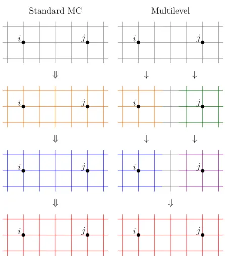
The multilevel algorithm is sketched in Fig. 2.1. In the standard Monte Carlo simulation the complete lattice is updated in every step and a correlator is measured. The error scales as N^−1/2. In the multilevel algorithm the complete lattice is updated only every f-th step. Between the big updates, the two subvolumes – each containing one operator of the correlator – are updated independently with a layer of the lattice fixed as boundary condition between the two subvolumes. Such updates are possible for a local lattice action. The correlator only depends on the fields on the boundary and therefore can be calculated also after averaging the operator measurements on the independently updated configurations. This reduces the statistical error on each correlator measurement by a factor of f⁻^1/2. The correlator is then only averaged over N/f averages of the measured operators. But in total, the error then scales approximately as (N/f)^−1/2(f^−1/2)² = (f N)^−1/2, which means that it can be a factor of f^−1/2 smaller. This significant error reduction is only valid if a large part of the statistical error comes from the short distance fluctuations around an operator in one compartment. This strategy has been used successfully for pure Yang-Mills theory in [62, 66, 67, 70]. For full QCD with dynamical quarks this prescription cannot be applied, because the action is non-local due to the fermion determinant.

Smearing prescriptions on the other hand do not modify the simulation but instead the measurement of the observables and are independent of the locality of the action. The effect of smearing is sketched in Fig. 2.2. Smearing also averages over short distance fluctuations in the measurement of the observables, from which correlators can be built, like the multilevel algorithm. But unlike the multilevel algorithm, smearing averages over the short distance fluctuations on a single configuration rather than over the fluctuations over configurations separated in simulation time. Smearing can be implemented in two different ways: One can construct an operator which is extended over a larger range of the lattice and is not local anymore or one can construct a lattice of smeared links which incorporate the information of their unsmeared neighbours and measure the standard local operators on them.³ As smearing makes the operators non-local, the results are not identical to the ones obtained in continuum theory with local operators. They are

2This ”multilevel algorithm” has nothing to do with the ”multilevel method” or ”multigrid method” to invert the lattice Dirac operator explained in e.g. [41, 42]

3The smearing described here is different from the smearing in the action, which is used to improve scaling properties of the action. The smearing here is only applied for the measurement on configurations generated with any action, smeared or unsmeared.

(20)

Standard MC

i j

⇓

i j

⇓

i j

⇓

i j

Multilevel

i j

↓ ↓

i j

↓ ↓

i j

⇓

i j

Figure 2.1: The multilevel algorithm compared to the standard Monte Carlo procedure. For details see main text.

(21)

⇓

Figure 2.2: The effect of smearing on the measurement of an operator compared to the unsmeared counterpart. For details see main text.

some observable with the same quantum numbers but without the short distance contributions. To obtain the proper observable in the continuum limit and to recover the full ultraviolet contributions, one has to apply the smearing with an effective smearing radius which vanishes in the continuum limit.

A widely used smearing procedure is stout smearing [75]. Like all gauge smearing procedures stout smearing is a prescription how to average over a local set of gauge links to produce a smeared or ”fat” link. This new link U_µ⁰ is a function of the old links Uµ and defined as

U_µ⁰ =e^iQ^µUµ, (2.16)

Qµ =i 2

Ω^†_µ−Ωµ−1

3tr[Ω^†_µ−Ωµ], (2.17) Ωµ =



ρStout

X

ν6=µ

Cµν



U_µ^†, (2.18)

with Cµν being the staple in the µν plane. One can of course iterate the smearing procedure NStout times to produce even smoother field configurations. The resulting smearing radius is then given by

rsmear =a^q8ρStoutNStout. (2.19)

The smearing used in this thesis is stout link smearing, if not stated differently.

(22)

2.1.4 Finite Temperature Spectral Representation

Having defined lattice QCD as Euclidean field theory on a finite and discretized space time suitable for numerical treatment in the computer, it is now important to know how the Euclidean observables in these simulations relate to the Minkovski observables of real physics. In this context one often introduces spectral representations or spectral functions. This section presents some relations of thermal field theory which are important to understand the measurements done on the lattice.

For a more detailed discussion the references [14] and [57] can be recommended.

In this presentation only the bosonic case is considered as this case applies to all the correlators of the energy momentum tensor which will be the main observables in this thesis. Most concepts carry over to the fermionic case and whenever important formulae are derived and needed in the thesis, they will be stated in the fermionic version as well.

Given two bosonic field operators ˆφi(x) and ˆφj(x) at Minkovski space time point x= (t, ~x) = (x⁰, ~x) one can define the usual Green’s functions and correlators

Π^>_ij(q) = ^Z dtd³~xeîq^·^x^Dφî(x)ˆφ^†_j(0)Ê (2.20) Π^<_ij(q) = ^Z dtd³~xeîq·x^Dφˆ^†_j(0)ˆφ_i(x)Ê (2.21) Π^R_ij(q) = i

Z dtd³~xeîq·x^Dhφî(x),φˆ^†_j(0)ⁱθ(t)Ê (2.22) ρij(q) = ^Z dtd³~xeîq^·^x

1 2

hφˆi(x),φˆ^†_j(0)ⁱ (2.23) with Π^R_ij(q) called the retarded correlator,ρij(q) the spectral function, the Minkovski momentum q = (q⁰, ~q) = (ω, ~q), and the Heaviside function θ.

In Euclidean space one can only measure the Euclidean correlator Π^E_ij(˜q) =^Z ^β

0 dτd³~xeî˜^q·˜^x^Dφî(˜x)ˆφ^†_j(0)Ê (2.24) where ˜q = (i˜q0, ~q) is an Euclidean momentum, ˜x = (−iτ, ~x) = (−i˜x0, ~x) is an Euclidean position, and β = 1/T the inverse temperature.

From these definitions and the integral representation of the Heaviside function θ(t) =i

Z _∞

−∞

dω 2π

e⁻^iωt

ω+i0⁺ (2.25)

one finds the relation for the retarded correlator and the spectral function Π^R_ij(q) =^Z ^∞

−∞

dp⁰ π

ρij(p⁰, ~q)

p⁰ −q⁰+i0⁺. (2.26)

(23)

Using

1

∆±i0⁺ =P

1

∆

∓iπδ(∆) (2.27)

with the principal value P gives then the simple relation

=Π^R_ij(q) =ρij(q). (2.28)

Also, by plugging in the definition of the thermal expectation value and of the Heisenberg operators

h.i=T r^he⁻^β^H^ˆ.ⁱ (2.29) O(t, ~x) =ˆ e^it^H^ˆO(0, ~x)eˆ ⁻^it^H^ˆ (2.30) and inserting complete sets of energy eigenstates into the definitions of Π^>_ij(q) and Π^<_ij(q), one gets a Kubo-Martin-Schwinger (KMS) relation between them

Π^>_ij(q) =e^βq⁰Π^<_ij(q). (2.31) This directly relates them also to the spectral function

ρij(q) = 1 2

Π^>_ij(q)−Π^<_ij(q) (2.32)

= 1 2

1−e⁻^βq⁰Π^>_ij(q). (2.33) By inverse Fourier transformation of Equ. (2.20) and analytic continuation of the field operators one can additionally show for the spatially Fourier transformed Euclidean correlator

C(τ, ~q) :=^Z d³~xeî~^q^·^~^x^Dφî(˜x)ˆφ^†_j(0)Ê (2.34)

=^Z d³~xe^i~^q^·^~^x

Z d⁴p

(2π)⁴e⁻^ip^·˜^xΠ^>_ij(p) (2.35)

=^Z ^∞

−∞

dp⁰

2π e^−p⁰^τΠ^>_ij(p⁰, ~q) (2.36)

=^Z ^∞

−∞

dp⁰ π

e⁻^p⁰^τ

1−e^−βp⁰ρij(p⁰, ~q) (2.37) Plugging this into the defining equation of the Euclidean correlator Equ. (2.24) and performing the τ integral one arrives at

Π^E_ij(˜q) =^Z ^∞

−∞

dp⁰ π

ρij(p⁰, ~q)

p⁰−iq˜₀ . (2.38)

(24)

If ˆφi = ˆφ^†_j, which is true in many cases of interest, the spectral function is antisymmetric in p⁰ → −p⁰ and Equ. (2.37) can be simplified to

Ch(τ, ~q) =^Z ^∞

0

dω π

cosh^β₂ −τω

sinh^β₂ω ρij(ω, ~q). (2.39) This equation can be understood as a finite temperature and continuous spectrum generalization of the basic Equ. (2.4). It is essential for lattice studies of spectral properties of a theory as it connects the spectral function of Minkovski space-time on the right hand side with an observable which is directly accessible in Euclidean space-time on the left hand side. In principle, an accurate measurement of the left hand side followed by inversion of the integral transformation can yield the spectral function. However, this inversion leads to a lot of technical problems as discussed in detail in section 3.3.

Equs. (2.37) and (2.39) are valid for bosonic operators. This already covers a large class of interesting observables including bilinears of fermionic operators which couple to mesons. For baryons one needs the analogous relation for fermionic operators which read

C^F(τ, ~q) :=^Z ^∞

−∞

dp⁰ π

e⁻^p⁰^τ

1 +e⁻^βp⁰ρij(p⁰, ~q) (2.40) C_h^F(τ, ~q) :=^Z ^∞

0

dω π

sinh^β₂ −τω

sinh^β₂ω ρij(ω, ~q). (2.41) These are the same relations as for bosonic operators up to a sign. This sign is exactly the sign difference between the Bose-Einstein and Fermi-Dirac distribu- tions and cause the difference in statistics. Equ. (2.41) is again valid for operators which satisfy ˆφi = ˆφ^†_j.

In later parts of the thesis the spatially Fourier transformed Euclidean correlators C(τ, ~q) will be called simply Euclidean correlators as the completely Fourier transformed Euclidean correlators Π^E(˜q) will not appear again.

2.2 Energy Momentum Tensor and Transport

As stated in the introduction, strongly interacting matter at high energies is in a quark gluon plasma state. This state behaves in first approximation more like an interacting fluid than a gas of quasi free particles. To describe such a medium in relativistic parameter regions the language of relativistic hydrodynamics can be used. In experiments at heavy ion colliders it was determined that the medium created in such collisions in fact behaves like a nearly perfect fluid. Relativistic

(25)

hydrodynamics is formulated in terms of one of the most basic observables of any physical theory, the energy momentum tensor.⁴

2.2.1 Energy Momentum Tensor

The energy momentum tensor is a symmetric⁵ tensor field Tµν(x) atx= (τ, ~x). It is the conserved Noether current associated with space-time translations

∇νT^µν(x) = 0. (2.42)

On the diagonal, its entries are the energy density T⁰⁰ = and the pressure Tⁱⁱ = P. The off diagonal elements are the momentum density T⁰ⁱ = Tⁱ⁰ and the shear stress or momentum flux T^ij = T^ji. As only flat Euclidean space-time is considered in most parts of this thesis, usually there is no distinction made between covariant and contravariant indices and covariant and partial derivatives.

For pure gauge theories it is given as Tµν(x) =Fµσ(x)Fνσ(x)−1

4δµνFρσ(x)Fρσ(x), (2.43) where Fµν(x) is the field-strength tensor and a trace over the suppressed color indices is understood. This expression is traceless in the classical theory. In quantum theoryFµσFνσ andFρσFρσ renormalize differently and there is a contribution to the trace from the conformal anomaly. Most observables built from the energy momentum tensor, which are considered in this thesis, are built from the traceless part Θµν of the full T_µν only. Therefore in the following the renormalization of the traceless contribution is discussed only. A method to renormalize the trace part will be discussed separately in section 2.3.5.

General Non-perturbative Anisotropic Renormalization Strategy This prescription is quite general and is therefore discussed for a general setting.

In the end it uses an existing set of renormalization factors of the isotropic lattice to determine the absolute scale of renormalization factors.

Let O_i be a set of N multiplicatively renormalizable observables⁶, ˆO_i the corresponding set of discretized operators for theOi, andZi a set of renormalization

4Some authors prefer the term ”stress tensor” instead of ”energy momentum tensor”.

5In most cases of relevance, like the standard model and general relativity, the energy momentum tensor is symmetric. There are, however, exceptions to this rule, e.g. in generalizations of general relativity like Einstein-Cartan theory.

6This is not a restriction of this prescription as one can always find a basis of multiplicatively renormalizable observables.

(26)

factors such that

hO_ii=Z_ihOˆ_ii. (2.44) In general, the renormalization factors and the lattice expectation values of the discretized operators depend on the discretization, while the observables are discretization independent.

Z_i =Z_i(a, ξ), (2.45)

hOˆii=hOˆii(a, ξ), (2.46)

Oi =Oi. (2.47)

As the observables do not depend on the discretization, they have in particular to be equal for different choices of the discretization⁷, e.g. for different anisotropies⁸. This gives us

hOii=Zi(ξ0)hOˆii(ξ0)

=Zi(ξ1)hOˆii(ξ1). (2.48) As one can measure the discretized expectation values, Equ. (2.48) is sufficient to measure at any given temperature the ratios of the renormalization factors Zi(ξ0)/Zi(ξ1), provided that the expectation value of the observables is not zero (as is the case for the energy momentum tensor).

But also the case of vanishing expectation values can be resolved. The simplest option is to use correlators at a finite physical distance.

Letoi(x) be the four-density corresponding to the operator Oi, i.e.

Oi =^Z d⁴xoi(x), (2.49)

and ˆo_i(x) the discretized density. Both have the same renormalization constant Zi

ho_i(x)i=Z_ihoˆ_i(x)i. (2.50) Then one can construct N(N + 1)/2 independent correlators Cij(τ)⁹ which are

7This statement is strictly true only in the continuum limit. In the following it is assumed that the lattices are fine enough.

8As only the case of different anisotropies is covered here, the lattice spacing argument ais dropped in the following.

9This can also be done with correlators separating the operators in spatial direction.

(27)

new observables still only depending on the same N renormalization factors Zi. The correlators may be defined as

Cij(τ) :=^Z d³h~xoi(x)oj(0)i (2.51)

=ZiZ_j

Z d³~xhˆo_i(x)ˆo_j(0)i. (2.52) Like the observables Oi, their correlators Cij(τ) are independent of the discretization, their discretized densities, however, are again discretization depen- dent:

Cij(τ) = Cij(τ) (2.53)

ˆ

oi(x) = ˆoi(ξ, x) (2.54)

Following the same arguments which lead to Equ. (2.48) one gets here Cij(τ) = Zi(ξ0)Zj(ξ0)^Z d³xhoˆi(x)ˆoj(0)i(ξ0)

=Z_i(ξ1)Zj(ξ1)^Z d³xhoˆ_i(x)ˆo_j(0)i(ξ1). (2.55) Equ. (2.55) is now an overdetermined system of equations for the ratios of renormalization factors Z_i(ξ0)/Zi(ξ1) which allows for a fit of these ratios. The choice of τ for this system sets the renormalization scale.

Having determined the ratios of renormalization factors non-perturbatively, of course one still has to get the absolute scale of the factors. For this it is usually the most convenient choice to simulate using an isotropic reference lattice because usually some of the factors are degenerate. Such a case allows also for the determination of ratios between some of the anisotropic renormalization factors and to build some observables which do not renormalize multiplicatively in the anisotropic but in the isotropic setting. For all other observables and to get the absolute scale of the renormalization factors one needs the isotropic factors from somewhere else.

Renormalization Structure of the Energy Momentum Tensor On the isotropic lattice the renormalized traceless energy-momentum tensor is

Θîso_µν =Z_µνîsoθîso_µν (2.56)

θîso_µν =F_µσîsoF_νσîso− 1

4δ_µνF_ρσ^isoF_ρσ^iso, (2.57)

(28)

where Z_µνîso =Z^diag for µ=ν, Z_µνîso =Z^rest for µ 6=ν, and F_µνîso is a discretization of the field-strength tensor on an isotropic lattice.

On the anisotropic lattice this has to be modified introducing different renormalization factors depending on the anisotropy ξ =as/at. The operators have to be built from irreducible representations of the remaining cubic symmetry group of the lattice. Every representation gets its individual renormalization factor. The relevant building blocks in terms of quadratics of the anisotropic field strength tensor F_µν^iso are given in Tab. 2.1.

operators E and B Z factor

P

i F_0iîso² ^P_iE_i² ZÊE⁰ F_0iîso²− F_0jîso² E_i² −E_j² ZÊE¹ F_0iîsoF_0jîso EiEj ZÊE²