Magnetic susceptibility of QCD matter and its decomposition from the lattice

JHEP07(2020)183

Published for SISSA by Springer

Received: May 1, 2020 Revised: June 25, 2020 Accepted: June 25, 2020 Published: July 24, 2020

Magnetic susceptibility of QCD matter and its decomposition from the lattice

Gunnar S. Bali,^a,b Gergely Endr˝odi^c,d and Stefano Piemonte^a

aInstitut f¨ur Theoretische Physik, Universit¨at Regensburg, D-93040 Regensburg, Germany

bTata Institute of Fundamental Research, Homi Bhabha Road, Mumbai 400005, India

cInstitut f¨ur Theoretische Physik, Goethe Universit¨at Frankfurt, D-60438 Frankfurt am Main, Germany

dFakult¨at f¨ur Physik, Universit¨at Bielefeld, D-33615 Bielefeld, Germany

E-mail: gunnar.bali@ur.de,endrodi@physik.uni-bielefeld.de, stefano.piemonte@ur.de

Abstract: We determine the magnetic susceptibility of thermal QCD matter by means of first principles lattice simulations using staggered quarks with physical masses. A novel method is employed that only requires simulations at zero background field, thereby cir- cumventing problems related to magnetic flux quantization. After a careful continuum limit extrapolation, diamagnetic behavior (negative susceptibility) is found at low temper- atures and strong paramagnetism (positive susceptibility) at high temperatures. We revisit the decomposition of the magnetic susceptibility into spin- and orbital angular momentum- related contributions. The spin term — related to the normalization of the photon lightcone distribution amplitude at zero temperature — is calculated non-perturbatively and extrap- olated to the continuum limit. Having access to both the full magnetic susceptibility and the spin term, we calculate the orbital angular momentum contribution for the first time.

The results reveal the opposite of what might be expected based on a free fermion picture.

We provide a simple parametrization of the temperature- and magnetic field-dependence of the QCD equation of state that can be used in phenomenological studies.

Keywords: Lattice QCD, Lattice Quantum Field Theory, Phase Diagram of QCD, Quark- Gluon Plasma

ArXiv ePrint: 2004.08778

JHEP07(2020)183

Contents

1 Introduction 1

2 The response of QCD matter to background fields and the magnetic

susceptibility 2

2.1 QED renormalization 3

2.2 The tensor coefficient 4

2.3 Decomposition into spin and orbital angular momentum contributions 5

3 Lattice methods 6

3.1 Magnetic flux quantization 7

3.2 Determining the susceptibility via current-current correlators 8

4 Results 10

4.1 The magnetic susceptibility 12

4.2 The normalization of the photon distribution amplitude 15

4.3 The spin contribution at T >0 18

4.4 Pauli and Landau decomposition of the magnetic susceptibility 21

5 Summary 21

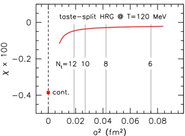
A The HRG model and lattice discretization errors 23 B Separation into quark spin and other angular momentum contributions 24

C Susceptibilities in the free case 26

C.1 Magnetic susceptibility 26

C.2 Ultraviolet divergences and QED renormalization 27

C.3 Spin contribution 28

C.4 Tensor bilinear 28

C.5 High-temperature expansion 29

D Multiplicative QCD renormalization 30

E Susceptibilities via current-current correlators 32

E.1 Magnetic susceptibility from correlators 32

E.2 Tensor coefficient from correlators 34

F Parametrization of the equation of state 35

JHEP07(2020)183

1 Introduction

The development of a quantitative and precise understanding of the response of QCD matter to background (electro)magnetic fields is of vital importance for furthering our knowledge about a multitude of physical systems. Examples include the interior of mag- netars, neutron star mergers [1–3], off-central heavy-ion collisions and the evolution of the universe in its early stages. For general reviews, we refer the reader to refs. [4–6]. A characteristic feature of the behavior of strongly interacting quarks and gluons is rooted in the dependence of the QCD equation of state (EoS) on the background magnetic field B.

The EoS enters all the above mentioned examples: it appears in the gravitational stability conditions of compact stars, affecting the mass-radius relation [7]; it governs the expansion rate in cosmological models [8,9] and it also sets the conditions where freeze-out is reached in heavy-ion collisions, see, e.g., ref. [10].

While the equilibration of fireballs produced in heavy-ion collisions is still a subject of research, at least in astrophysical systems the time and distance scales over which the magnetic field varies are much larger than those that govern QCD processes that affect, e.g., the EoS or nucleo-synthesis. With these applications in mind, solving QCD in a constant background magnetic field is sufficient and this scenario is amenable to lattice simulations.

The leading dependence of the EoS on B is encoded in the magnetic susceptibilityχof QCD matter. Its sign distinguishes between paramagnets (χ >0), for which the exposure to the background field is energetically favorable, and diamagnets (χ <0), which repel the external field. In QCD matter, like in any other material, the origin of the magnetization and hence of the magnetic susceptibility is related to the spin and angular momentum of charged particles. At high temperatures the quarks are the relevant degrees of freedom;

at low temperatures the hadrons and in particular the pions take over, while (valence and sea) quarks contribute just as their fundamental constituents.

The total angular momentum that gives rise to the magnetization can be decomposed into contributions from the spins of the quarks of different flavors and a remainder. The latter contains the quark orbital angular momenta but also the angular momentum of the gluons, that can split into quark-antiquark pairs.¹ The quark spin contribution to the magnetic susceptibility is due to the expectation value ψ¯fσµνψf

, whose leading order re- sponse is linear in the magnetic field strength tensorF_µν. Depending on the normalization, the slope is proportional to the magnetic susceptibility of the quark condensate [14–16], or the so-called tensor coefficient, i.e. the normalization of the photon lightcone distribution amplitude (DA) [17–19] of finding a quark-antiquark pair of flavorf in a transverse photon.

This in itself appears in a multitude of applications, e.g., as a correction to the hadronic

1This situation is analogous to the decomposition of the nucleon spin. In particular, vacuum expectation values of the same local operators appear in the magnetic field background at zero momentum as in the decomposition [11] of the transversely polarized generalized parton distribution functions of deep inelastic scattering at leading twist. While the individual quark spin contributions in both cases are unique and gauge invariant, the further decomposition of the remainder into quark and gluon parts is ambiguous: the decomposition of ref. [11] is based on the Belinfante-Rosenfeld form of the energy momentum tensor, which is also the natural starting point for lattice QCD, but one may also, e.g., resort to the canonical definition of the angular momentum [12,13].

JHEP07(2020)183

light-by-light scattering contribution to the muon anomalous magnetic moment [20, 21], within radiative transitions [22,23] and in the photo-production of mesons [24].

Some of the present authors have already addressed several of the above aspects in refs. [25–28]. Here we improve on these studies by employing a novel calculational method that is based on ref. [29], by carrying out the QCD renormalization non-perturbatively with respect to the intermediate RI’-MOM scheme [30, 31] and by adding a finer lattice spacing. In addition we present and exploit new analytical findings. One of the outcomes will be that in the strongly interacting medium at low to moderately high temperatures the quark spin-related susceptibility is negative (diamagnetism) while the part that is due to the orbital angular momentum is positive. Clearly, this behavior is very different from the response to magnetic fields of the materials that have so far been accessible to solid state physics experiments. Therefore, our results offer a glimpse into a completely new regime of spin physics.

The article is organized as follows. In section2we introduce our notations and the cen- tral observables. For conceptual clarity, we carefully address their divergence structure and renormalization in QED and QCD. In section 3 we then discuss details of the simulation and, in particular, we introduce our new method that employs current-current correlators in a mixed coordinate- and momentum-space representation. This enables us to determine susceptibilities from lattice simulations at B= 0. We then present and discuss our results in section4, before we summarize. We include several technical appendices: in appendix A we investigate the effects of taste splitting in the staggered formulation within the hadron resonance gas model. This turns out to be important to avoid underestimating the sys- tematics of the continuum limit extrapolation. In appendix B we derive the factorization of the susceptibility into quark spin-related and other contributions, building upon earlier partial results [26]. In the extensive appendixC, several derivations are carried out for the free case, establishing, e.g., the structure of QED divergencies. Appendix D discusses the non-perturbative renormalization procedure. In appendix Ewe present more detail on the derivation of the new current-current method and compare to numerical results, obtained using conventional background field approaches. Finally, appendix Fgives a parametriza- tion of our results for the QCD EoS for a broad range of temperatures and magnetic field strengths. The corresponding Python script param EoS.py is uploaded as Supplementary material along with this paper.

2 The response of QCD matter to background fields and the magnetic susceptibility

Without any loss of generality, below we consider a magnetic field pointing in the x3

direction, with the magnitude B. The magnetic susceptibility is defined via the leading (quadratic) dependence of the QCD free energy density f on the field strength,

χ_b =− ∂²f

∂(eB)² B=0

, f =−T

V logZ, (2.1)

where Z is the partition function, T the temperature and V the spatial volume of the system. The product eB of the elementary electric charge e and the magnetic field is a

JHEP07(2020)183

renormalization group invariant due to the QED vector Ward identity, see eq. (2.3) below.

Therefore, χb is free of multiplicative renormalization. Still, the susceptibility undergoes additive renormalization, which is made explicit by the indexb, indicating the bare quantity, as obtained in the lattice scheme at a lattice spacing a.² This was discussed in ref. [28] in depth, but we repeat the argument here for comprehensiveness.

2.1 QED renormalization

The total free energy density of the system, that includes both QCD matter and the classical background field,

f_tot=f +B_b²

2 , (2.2)

is a physical observable and therefore free of divergences. However, the second term within eq. (2.2), involving the bare magnetic field B_b, contains a logarithmic divergence in the lattice spacingadue to electric charge renormalization [32],

B_b² =ZeB², e²_b =Z_e⁻¹e², eB=e_bB_b, Ze= 1 +β1(a⁻¹)e² log µ²_QEDa² , (2.3) where the renormalized quantities e and B depend on the QED renormalization scheme and on the QED renormalization scale µ_QED. Since the background field is classical, only the leading-order QEDβ-function coefficientβ₁ appears here [33]. Note that β₁ is affected by QCD corrections at the cut-off scale,

β₁(a⁻¹) =β₁·

"

1 +X

i≥1

c_ig²ⁱ(a⁻¹)

#

−−−→a→0 β₁, β₁= 1 4π² ·X

f

(q_f/e)², (2.4) where g is the strong coupling and q_f denotes the electric charge of the quark flavor f.

The coefficients ci of the perturbative series are known up to i= 4 in the MS and MOM schemes [34] andc₁ = 1/(4π²) is universal for massless schemes. These QCD corrections³ vanish logarithmically with the lattice spacing towards the continuum limit due to the asymptotically free nature of the strong interactions, as is also indicated in eq. (2.4).

Eq. (2.2) implies that f contains the same additive divergence as B_b²/2, but with an opposite sign. This propagates into the susceptibility (2.1), resulting in

χ_b=χ[µ_QED] +β₁(a⁻¹) log(µ²_QEDa²). (2.5) The renormalized susceptibilityχdepends on the renormalization scale, which we indicated here explicitly in square brackets. We confirm the presence of the logarithmic divergence in χ_b analytically for the free case in appendixC.2and numerically for full QCD in section4.1.

The divergence is independent of the temperature so that it cancels within the difference χ≡χ[µ^phys_QED] =χ_b(T)−χ_b(T = 0). (2.6)

2Below we will indicate quantities that are subject to QED renormalization with the subscriptb.

3Note that in general disconnected diagrams also start to contribute for i≥3, but in the present case these vanish because we are dealing with the three lightest quark flavors andP

fqf/e= 0.

JHEP07(2020)183

This definition of the renormalized susceptibility — implying that it vanishes identically at T = 0 — corresponds to a particular choice of the renormalization scale µQED=µ^phys_QED. In fact this is the only prescription that adheres to the physical requirement that the magnetic permeability (1−e²χ)⁻¹ should be unity in the vacuum. In the following we suppress the dependence on the QED renormalization scale and simply write χ for the susceptibility, renormalized in this way.

2.2 The tensor coefficient

Besides the magnetic susceptibility there exist further quantities that characterize the leading-order response of the QCD medium to the background magnetic field. For a gen- eral background field Fµν, the fermion bilinear involving the relativistic spin operatorσµν

develops a nonzero expectation value [14,35], ψ¯_fσ_µνψ_f

=q_fF_µν·τ_{f b}+O(F³), σ_µν = 1

2i[γ_µ, γ_ν]. (2.7) We will refer to τf b as the tensor coefficient for the flavor f. Similarly toχb, this is also a bare observable that contains additive logarithmic divergences in the cut-off. For our choice of direction of the magnetic field the tensor coefficient can be determined as the slope of the expectation value of the fermion bilinear involving σ12 at small values of the magnetic field:

τ_{f b}= lim

B→0

ψ¯_fσ₁₂ψ_f

qfB . (2.8)

The tensor coefficient contains a similar logarithmic divergence asχ_b. We demonstrate the reason for this in section 2.3 below. In particular, the divergence structure takes the form [26],

τ_{f b}=τ_f+γ₁^τ(a⁻¹)m_flog(µ²_QEDa²), γ₁^τ(a⁻¹) =γ₁^τ·

1 +O(g²(a⁻¹))

, γ^τ₁ = 3 4π² ,

(2.9) where mf is the mass of the quark of flavor f. Again, due to asymptotic freedom, QCD corrections to γ₁^τ vanish in the continuum limit.⁴ Eq. (2.9) is confirmed in appendix C.4 for the free case and checked numerically in full QCD in section 4.2. Notice that in the chiral limit the divergent term disappears, so that limmf→0τ_{f b} is ultraviolet-finite. We will carry out this limit at zero temperature in section 4.2 below. In this situation, up to multiplicative renormalization, this object corresponds to the normalization f_γ^⊥ of the leading-twist photon distribution amplitude [17–19], i.e. of the infinite momentum frame probability amplitude that a real photon dissociates into a quark-antiquark pair of flavorf.

In analogy to eq. (2.6), we define the renormalized tensor coefficient by subtracting its value at zero temperature,

τ_f =τ_{f b}(T)−τ_{f b}(T = 0), (2.10)

4Unlike forβ1(a⁻¹) in eq. (2.4), the orderg²perturbative coefficient is not known in this case. Therefore, any definition of a renormalized quark massmf is valid to this order and we use the lattice quark mass.

JHEP07(2020)183

which again corresponds to a particular choice of the QED renormalization scale. Unlike forχ, there is no preferred choice in this case, but it is natural to use the same prescription as in eq. (2.6) above.

Besides the (QED-related) additive renormalization detailed above, the tensor coef- ficient also undergoes (QCD-related) multiplicative renormalization by the tensor renor- malization constant Z_T. This introduces a further scheme- and scale-dependence of this observable. Below we will considerZT in the MS scheme at the QCD renormalization scale µQCD= 2 GeV. Unlike in our previous study [26], where we calculated ZT perturbatively at the one-loop level, here we carry out a non-perturbative matching to the RI’-MOM scheme [30,31] and subsequently translate the result at three-loop order [36] into the MS scheme. This procedure is detailed in appendix D. We remark that Z_T is independent of the temperature, thus the ordering of the QED renormalization (i.e. theT = 0 subtraction) and the QCD renormalization (multiplication byZT) is irrelevant for the determination of the renormalized tensor coefficient τ_f.

2.3 Decomposition into spin and orbital angular momentum contributions One might suspect thatχandτ_f are not completely unrelated. Indeed, as we first discussed in ref. [26], τf represents the contribution of the spin of the quark flavor f to the total magnetic susceptibility. In particular, χ can be decomposed into spin-related and orbital angular momentum-related contributions,⁵

χ=χ^spin+χ^ang, (2.11)

and the spin term is related to the tensor coefficients as χ^spin=X

f

(qf/e)² 2m_f

h

τ_f(m^val_f )−τ_f(m^val_f →0)i

·Z_TZ_S, (2.12) wherem_f denotes the quark mass in the lattice scheme and Z_S and Z_T are the scalar and tensor renormalization constants, respectively. The second term in the square brackets is understood to correspond to the limit of a vanishing valence quark mass taken at physical, i.e. nonzero, values of the sea quark masses. We discuss the difference between valence and sea quark masses in section 3 below. In appendix B we prove eqs. (2.11)–(2.12) and illustrate the origin of the subtraction of the chiral valence quark limit. Appendix C also contains an explicit check of eq. (2.12) in the free case.

A remark regarding the choice of renormalization scales is in order here. Eq. (2.12) is chosen so that χ^spin vanishes atT = 0. Recall however that, according to our remark below eq. (2.10), we are free to choose an arbitrary QED renormalization scale for the renormalized tensor coefficient. This freedom propagates into χ^spin and — through the decomposition (2.11) — toχ^angas well. In contrast, the renormalization scale forχis fixed by the requirementχ(T = 0) = 0. Thus, in principle both susceptibility contributions may

5Note that for simplicity we refer toχ^angas the orbital angular momentum contribution. In the interact- ing case this can be further factorized, separating out the gluon total angular momentum contribution [27]

from those of the quark angular momenta.

JHEP07(2020)183

be shifted by an arbitrary amount, as long as their sum remains zero at T = 0. We will follow the choice made in eq. (2.12), which corresponds to settingχ^spin(T = 0) =χ^ang(T = 0) = 0. In the free case this is realized by choosingone and the same QED renormalization scale for all susceptibility contributions, see appendix C.3. Our numerical results in full QCD below suggest that also in the interacting case the QED scale that corresponds to the renormalization condition χ^spin(T = 0) = 0 is consistent with the one obtained from setting χ(T = 0) = 0.

In eq. (2.12) we also carried out the QCD related multiplicative renormalization by including the tensor renormalization constant ZT required forτ_f (as mentioned above) as well as the scalar renormalization constant Z_S =Z_m⁻¹, which multiplies the inverse quark mass.⁶ Note that these renormalization factors depend on the QCD regularization scheme and on the QCD renormalization scale. As mentioned above, we choose the MS scheme andµ_QCD= 2 GeV. We remark that, just as forτ_f, the ordering of the QED and the QCD renormalization is irrelevant for χ^spin. We stress again that while the factorization of the total susceptibility χintoχ^spinand χ^ang depends on the QCD scheme and scale,χ itself is a QCD renormalization group invariant.

In the free case the two susceptibility contributions have a constant ratio,χ^spin:χ^ang= 3 : (−1), reflecting the well-known response of a free charged fermion to the magnetic field via its spin and its orbital angular momentum, dating back to Pauli and Landau [38,39].

This ratio, which translates into the ruleχ^spin:χ= 3 : 2, holds identically in the free case, see appendix C.3. In contrast, in full QCD it only applies to the divergence structure, which in the continuum limit — as we have seen above — is governed by pure QED physics. Below we determine to what extent the Pauli-Landau decomposition is affected by the strong interactions.

3 Lattice methods

We consider spatially symmetricN_s³×N_t lattice ensembles, corresponding to the temper- atureT = 1/(Nta) and the volumeV =L³= (Nsa)³. The simulations are performed with the tree-level Symanzik improved gauge action Sg and three flavors (f = u, d, s) of stout smeared rooted staggered quarks [40], described by the Dirac operator⁷ D/_f +m_f. The quark masses mf are tuned as a function of the inverse gauge coupling β = 6/g² along the line of constant physics: m_ud(β) ≡m_u(β) = m_d(β) =m_s(β)/R with R = 28.15 [41].

The electric charges are set as q_d = q_s = −q_u/2 = −e/3, where e > 0 is the elementary electric charge. The magnetic field enters inD/_f via space-dependent U(1) phases. Further details of our setup and of the simulation algorithm are discussed in ref. [42]. The lattice geometries for our finite temperature lattices are 16³ ×6, 24³×6, 24³ ×8, 28³×10 and 36³×12, allowing for the investigation of both finite volume and discretization effects. Our zero-temperature ensembles consist of 24³×32, 32³×48 and 40³×48 lattices.

6Like in massless continuum schemes, in staggered lattice formulations there is no difference between singlet and non-singlet renormalization factors for these quark bilinears. This was explicitly demonstrated at orderg⁴ in ref. [37].

7Due to the electromagnetic chargeqf, the covariant derivative depends on the quark flavorf.

JHEP07(2020)183

In the rooted staggered formulation the partition function and the expectation value of the tensor bilinear are written as path integrals over the SU(3)-valued gluonic links U as

Z= Z

DU e^−βSg Y

f⁰=u,d,s

det(D/_f⁰+m^sea_f⁰ )1/4

, ψ¯_fσ₁₂ψ_f

= T V

1 Z

Z

DU e^−βSg tr σ₁₂ D/_f +m^val_f

Y

f⁰=u,d,s

det(D/_f⁰+m^sea_f0 )1/4

.

(3.1)

Here we distinguished between two different types of masses: the sea quark masses m^sea_f which appear in the fermion determinant and thus affect the generation of gluonic configu- rations; and the valence quark mass m^val_f , which enters in the operator and thereby affects the measurement on a given set of configurations. For usual observables both masses are equal and set according to the line of constant physics, m^sea_f =m^val_f =mf. The spin con- tribution to the magnetic susceptibility is exceptional in this sense — as pointed out above in eq. (2.12), it also involves the value of ψ¯_fσ₁₂ψ_f

in the limit m^val_f → 0 but keeping m^sea_f =mf. Note that this does not mean that we are dealing with a non-unitary theory but merely that χ^spin can be expressed as a difference of two expectation values involving τ_f at different valence quark mass values, see appendixB.

3.1 Magnetic flux quantization

In an infinite volume a magnetic field pointing in the x3 direction can be generated by the Landau-gauge electromagnetic potential

A2=Bx1. (3.2)

In a finite volume, in order to comply with periodic boundary conditions for the electromag- netic parallel transportersu_µf= exp(iq_fA_µ), the boundary twist termA₁=−Bx₂L δ(x₁−L) needs to be included as well [43]. In this setup the flux of the magnetic field is quantized according to [44]

eB= 6πN_B/L², N_B ∈Z, (3.3)

so that a differentiation with respect to eB — as required in eq. (2.1) — is not possible in a standard manner. Several methods were developed to overcome this problem on the lattice, including the anisotropy method [27,45], the finite difference method [46,47] and the generalized integral method [28]. These are all based on approximating the derivative numerically using finite differences in the integer variable N_B. This requires independent simulations using several values of NB, which increases the computational requirements considerably. Furthermore, an extrapolation N_B→0 becomes necessary, which inevitably introduces systematic uncertainties. An alternative approach is the half-half method [48], which employs a magnetic field profile that is positive in one half and negative in the other half of the lattice — this enables taking the derivative with respect to the amplitude of the field analytically. However, finite volume effects are substantially enhanced in this case due to the discontinuity of the background field at the boundaries [29] — even if such effects are expected to cancel in temperature differences [49].

JHEP07(2020)183

3.2 Determining the susceptibility via current-current correlators

In view of the above, a method is desirable that only involves measurements at B = 0, thereby circumventing the flux quantization problem of the constant background field profile. In ref. [29] we demonstrated that at zero temperature, χb, as defined in (2.1), is related to a mixed-representation two-point function of the electromagnetic current, and can thus be measured atB = 0. Below we motivate this method and clarify how it extends to nonzero temperatures. A detailed derivation can be found in appendixEand, forT = 0, in ref. [29].

Before integrating out the fermions in the path integral (3.1), the vector potential (3.2) couples toi·etimes the µ= 2 component of the electromagnetic current,

j_µ=X

f

qf

e ψ¯_fγ_µψ_f, (3.4)

in the action density. Taking derivatives of logZ with respect to eB therefore brings down integrals over the current j₂ times the x₁-dependent term i ∂A₂/∂B. Thus we can anticipate the result to take the form of a convolution of the projected correlator,

G(x₁) = Z

dx₂dx₃dx₄ hj₂(x)j₂(0)i , (3.5) with an x1-dependent kernel.

Instead of directly using the gauge (3.2), it is instructive to approach the constant magnetic field background via oscillatory fields that possess nonzero momentum p1 in the x1 direction. Using these profiles, we can take the thermodynamic limit and subsequently the p₁ → 0 limit. This approach reveals that the magnetic susceptibility (2.1) arises as a smooth limit of susceptibilities with respect to oscillatory fields. As the details of the derivation are somewhat technical, we delegate them to appendix E and only quote the main results here.

In the thermodynamic limit, where the momentum variable is continuous and the p₁ →0 limit can be taken, the susceptibility is obtained as

χ_b =− lim

p1→0

Z

dx₁ cos(p₁x₁)−1

p²₁ G(x₁) = Z

dx₁ x²₁

2 G(x₁). (3.6) In finite volumes (x1 ∈[0, L]) the momentum variable p1 is discrete, so that the p1 → 0 limit does not exist. Nevertheless, we can safely employ the formula (3.6) directly in finite volumes, as long as the linear sizeLis much larger than the characteristic length governing the exponential decay ofG(x₁). Symmetrizing eq. (3.6) to comply with periodic boundary conditions and the symmetry G(x₁) =G(L−x₁), we arrive at

χb = 1 2

Z L

0

dx1G(x1)·

(x²₁, x1 ≤L/2

(x₁−L)², x₁ > L/2 . (3.7) In the representation (3.7) the current-current correlator is computed in coordinate space. Only afterwards a Fourier transformation is carried out via the convolution with

JHEP07(2020)183

the quadratic kernel in order to represent the constant background field. In this way the problem of flux quantization is avoided. Notice that there is a remnant of flux quantization in the formula (3.7), signaled by the cusp in the kernel atx₁ =L/2. However, this cusp has no practical relevance, as in the integral it is multiplied by G(L/2), which is exponentially small. Thus we do not expect to encounter substantial finite volume effects. This is contrary to the case of the half-half method [48], where translational invariance is broken already on the level of the expectation values, involving a vector potential with kinks. Nevertheless, we investigate the finite volume effects of the new method numerically in section 4.

The result (3.6) can be recast into an alternative form using the vacuum polarization tensor

Π_µν(p) = Z

d⁴x e^ipxhj_µ(x)j_ν(0)i , Π₂₂(p={p₁,0,0,0}) =−p²₁Π(p²). (3.8) The second relation, involving the vacuum polarization form factor Π, only holds for this specific choice of spatial indices.⁸ Employing these definitions, we can rewrite

χ_b = lim

p1→0 Π(p²) = Π(0), Π(p²) = Z

dx₁1−cos(p1x1)

p²₁ G(x₁), (3.9) where we used that the imaginary part of Π(p²) vanishes.

We note that the vacuum polarization function Π has been the subject of intense re- search as it appears in the hadronic contribution to the muon anomalous magnetic moment, see, e.g., the recent review [52]. In that setting the relevant observable is the second moment of the two-point function of the electromagnetic current (3.4), projected to zero spatial mo- mentum [53]. Exchanging the time coordinate x₄ for the spatial coordinate x₁, one can obtain χb in an analogous way in our background field setup [29]. The two determinations are equivalent at zero temperature. ForT >0 it is important to use spatial momenta, i.e.

a kernel involving spatial coordinates for χ_b, since this encodes the magnetic response.

In appendix E we derive a similar representation for τ_{f b} as well. In this case the equivalents of eqs. (3.5) and (3.7) become⁹

τ_{f b}= i q_f/e

Z L

0

dx1H_f(x1)·

(x1, x1≤L/2 x1−L, x1> L/2 , H_f(x1) =

Z

dx2dx3dx4

ψ¯_fσ12ψ_f(x)j2(0) .

(3.10)

We remark that the second moment of the photon DA is accessible too, replacing σ₁₂ by combinations of σ_µν←−

D_ρ←− D_σ+−→

D_ρ−→

D_σ −2←− D_ρ−→

D_σ

that are antisymmetric in indices equal

8At zero temperature, the second relation of eq. (3.8) follows directly from the decomposition Πµν(p) = (pµpν−δµνp²) Π(p²). For T >0 the Lorentz structure of Πµν(p) is more complicated so that, in addition to Π, a form factor ΠL appears [50,51]. However, in the static case (p4 = 0) only Π contributes to the spatial components of Πµν so that the second relation of eq. (3.8) continues to hold.

9On general grounds, the linear response of the expectation value of ann-point function with respect to a background field can always be obtained by computing (n+ 1)-point functions in the vacuum. Usually, the former method is favorable in terms of the statistical noise. However, the latter option exempts us from the need of generating additional gauge ensembles with non-vanishing values of the background field. As already discussed, in the present context, we also circumvent the issue of flux quantization.

JHEP07(2020)183

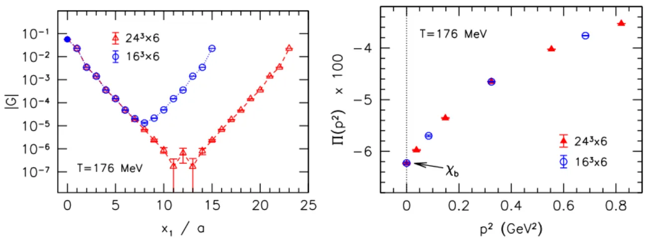
Figure 1. Left panel: comparison of the absolute value of the current-current correlator for two different volumes, 24³×6 (red) and 16³×6 (blue). Filled (open) points indicate positive (negative) values. Right panel: the vacuum polarization function at spatial momenta for T ≈176 MeV using two different volumes. The bare magnetic susceptibility can be read off from the intersect Π(0).

to 1 and 2, symmetrized over all other non-trivial combinations of indices and with all traces subtracted, see, e.g., ref. [54]. This is beyond the scope of the present work.

In summary, via the relation (3.7) we are able to determine the magnetic susceptibility using direct measurements at B = 0. This is certainly advantageous over calculating the free energy density (which cannot be obtained as a simple expectation value) at nonzero magnetic fields and differentiating it numerically. The similar relation for the tensor coef- ficient, eq. (3.10), might also be used to avoid measuring ψ¯_fσ₁₂ψ_f

at B >0. However, since the latter is a simple one-point function, the gain is not obvious in this case. In appendix E we compare the two methods for this observable and conclude that the corre- lator method indeed gives larger statistical errors. Therefore, we opted to use our earlier results [26] forψ¯_fσ12ψ_f

. 4 Results

First we demonstrate that — in accordance with eq. (3.9) —χ_b = Π(0) arises as a smooth limit of the vacuum polarization function Π(p²) at spatial momenta. To this end we calculate the correlatorG(x1) usingO(1000) random sources located on three-dimensional x₁-slices of our lattices, taking into account both connected and disconnected contributions.

The correlator is shown in the left panel of figure 1 for our N_t = 6 lattices at a high temperature T ≈ 176 MeV. Here we compare two different volumes with Ns = 24 and N_s= 16, revealing that finite size effects in the exponential fall-off are tiny. Subsequently, G(x₁) is convoluted with the kernels of eqs. (3.7) and (3.9) to obtain Π(0) and Π(p²), respectively. In the right panel of figure 1 we show Π(p²) for low momenta, again at the same temperature T ≈ 176 MeV. As expected, the zero-momentum limit is approached smoothly and the two volumes are found to agree perfectly.

Next we investigate finite volume effects in more detail. In particular, we truncate the convolution (3.7) at x^max₁ ≤ L/2 and plot the so-obtained truncated susceptibility

JHEP07(2020)183

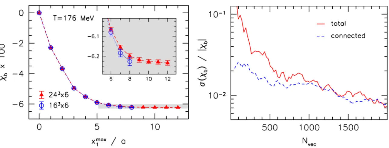
Figure 2. Left panel: the susceptibility obtained via a truncation of eq. (3.7) for two different volumes, 24³×6 (red) and 16³×6 (blue). The inset zooms into the region nearx^max₁ =Nsa/2. Right panel: relative error of the susceptibility as a function of the number of employed noisy estimators.

in the left panel of figure 2. This sheds more light on why volume effects are so small.

While for the smaller volume, the exponential decay is cut off at a lower x1, the slight enhancement of Garound L/2 due to the backward propagating exponential (see the left panel of figure 1) almost completely corrects for this. Finally, we estimated the deviation of the result from the thermodynamic limit by considering a single-exponential fit of the correlator at x₁ < L/2 and performing the convolution (3.6) for L/2 ≤ x₁ < ∞. For N_s = 16 this correction is found to be about half of the statistical error of χ_b, while for Ns = 24 it is found to be two orders of magnitude smaller than that. For these analyses we considered the results at T ≈176 MeV, where we have very precise data. For the lower temperatures our data are noisier; here we find the finite volume errors to be significantly smaller than our statistical uncertainties already for Ns = 16.

Before turning to the main results, we discuss the statistical accuracy and the numer- ical costs of the present method. The right panel of figure 2 shows the relative error of χb at T ≈113 MeV on our 24³×6 lattices as a function of the employed number Nvec of noisy estimators. The evaluation ofG(x₁) requires two inversions for the light quarks and two for the strange quark for each noisy estimator. The figure reveals that sub-percent errors can be achieved. For sufficiently high Nvec the connected contributions are found to dominate the error, as already recognized in ref. [29]. Alternative methods to calculate χ_b [28,46,47] require several independent simulations at nonzero B and a reconstruction of logZ for each magnetic field and are therefore much more expensive than the present approach (of course, in that case the physicalB >0 ensembles might also be used for other purposes). To be specific, we consider our results [28] using the integral method at the same temperature and lattice spacing as above. In that case we needed to perform around 40 independent simulations (at nonzero B as well as at different quark masses), generat- ing several hundred decorrelated configurations and measuring the quark condensate on each ensemble. We achieved a relative error of about four percent. More importantly, the present method outperforms previous alternatives because this determination of χ_b

JHEP07(2020)183

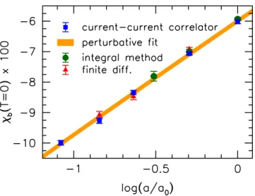
Figure 3. Bare magnetic susceptibility at zero temperature versus the logarithm of the lattice spacing, normalized toa₀ = 1.46 GeV⁻¹. Different approaches are compared: the finite difference method [47] (red triangles), the generalized integral method [28] (green circles) and the new ap- proach via current-current correlators (blue squares). The orange band indicates the fit based on perturbation theory, eq. (4.1).

entails no further systematic uncertainty, unlike approaches [28,46,47], where a numerical differentiation of logZ(B) is required.

4.1 The magnetic susceptibility

We compare the results of our new method for χ_b to our old data (generalized integral method) and also to those of ref. [47] (finite difference method) in figure 3 at zero tem- perature.¹⁰ Within errors perfect agreement between the three groups of results is found.

The data — plotted in figure3 against log(a) — clearly reflect the logarithmic divergence dictated by eq. (2.5). Similarly to our fitting strategy in ref. [29], here we also include the universal perturbative QCD corrections to the QED β-function coefficientc₁ [34], see eq. (2.4), whereg² = 6/β is obtained from the inverse lattice couplingβ at the lattice scale a⁻¹. We also take into account O(a²) lattice artifacts so that our fit function reads

χ_b = 2β₁(a⁻¹)·

log(a/a₀) + log(µ_QEDa₀)

·

1 +z₁(a/a₀)²

, a₀ = 1.46 GeV⁻¹. (4.1) The result of this fit, with the parameter values

µQED= 115(3)(5) MeV, z1=−0.05(1), (4.2) is shown as an error band in figure 3. We also considered fits with further (quartic) lattice artifacts. The impact of this is included in the second parentheses of eq. (4.2) for µ_QED as a systematic error. The renormalization scale agrees within errors with our earlier

10Ref. [47] employs the same lattice action. For a different action the bare susceptibilities would not only differ in terms of lattice artifacts but also by an additive constant, due to the different choice of renormalization scheme.

JHEP07(2020)183

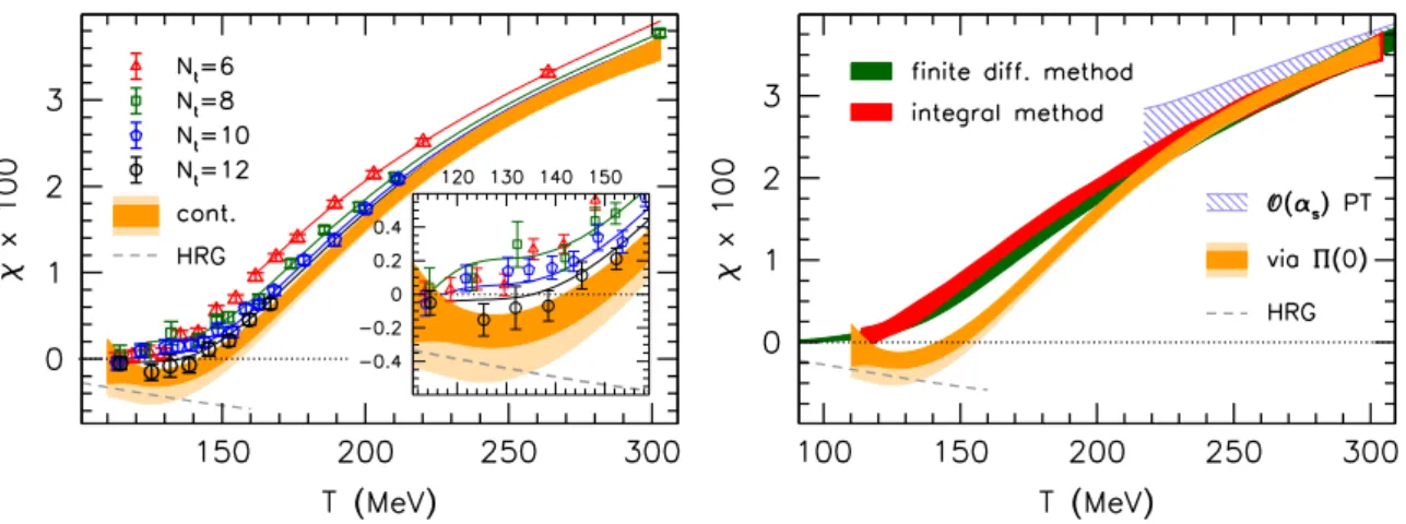
Figure 4. Left panel: renormalized susceptibility at nonzero temperature. The symbols indicate different lattice spacings and the dark orange band the continuum limit. The light orange band represents an estimate of systematic errors of the continuum extrapolation. The dashed gray line is the HRG model prediction [28]. The inset zooms into the low-temperature region to highlight the diamagnetic response there. Right panel: our results for χ (orange, labeled “via Π(0)”) are compared to the results of ref. [47] (green) and those of ref. [28] (red) as well as to the HRG model prediction (dashed gray line) and to perturbation theory [28] (dashed light blue band), see eqs. (4.3) and (2.4).

determinations [28, 29]. It also lies near the mass of the lightest charged hadron (the charged pion) which effectively sets the scale for the magnetic response of this system.

Nevertheless, note that the value of µ_QED depends on the choice of the regulator.

The formula (4.1) is used to interpolate χb and then employed to renormalize the susceptibility at nonzero temperatures according to eq. (2.6): χ = χ_b(T)−χ_b(0). The results are shown in the left panel of figure 4 for a broad range of temperatures and four lattice spacings a = 1/(NtT) with Nt = 6,8,10 and 12. A continuum extrapolation is performed by means of a multi-spline fit [55] taking into account O(a²) lattice artifacts.

To have acceptable fits of this type, we needed to discard the coarsest lattices (N_t= 6 points at T . 160 MeV). We also repeated the analysis including O(a⁴) discretization errors as well, this time fitting all available data points. The systematic error was estimated by the difference of these two extrapolations as well as by varying the spline node points and by including/excludingNt= 6 data points at high temperatures for theO(a²) fit. In addition, we consider a further systematic error due to lattice artifacts related to the taste splitting of the staggered spectrum. This effect is particularly relevant at low temperatures and can be estimated by a generalization of the Hadron Resonance Gas (HRG) model that we describe in appendixA. The light yellow bands in both panels of figure4indicate the total systematic uncertainties.

The results demonstrate strong paramagnetism in the quark-gluon plasma phase, in agreement with previous lattice studies [27,28,45–48]. At high temperatures the results are well described by the free theory, which predicts (see appendix C)

χ(T) =β₁(µ_therm)·log γ T² µ²_QED

!

+O(1/T²), (4.3)

JHEP07(2020)183

where γ = O(1) is a regulator-dependent constant.¹¹ As indicated, QCD corrections at the thermal scale µtherm affect the leading behavior. In the right panel of figure 4we also include a comparison to this perturbation theory formula, with the scheme-independent O(α_s) corrections to β₁ taken into account [28]. Here we set γ = 1 and use the MS scheme definition of the strong coupling αs=g²/(4π), running this at five-loop order [56]

to the thermal scale µ_therm ∼ 2πT. We employ the central value Λ^MS_QCD = 0.341 GeV from the recent three flavor QCD determination of αs by the ALPHA Collaboration [57].

The band in the figure corresponds to a variation of the thermal scale from πT to 4πT. The perturbative formula agrees surprisingly well with our results down to temperatures T ∼200 MeV.

In contrast to the paramagnetic behavior at high T, towards low temperatures the continuum extrapolated results become negative, revealing a diamagnetic response, previ- ously noted in ref. [28]. This behavior is in agreement, albeit within large errors, with the HRG model prediction [28] (dashed line in the figures). In the right panel of figure 4 we also include results obtained from other approaches that employed the same lattice action.

Around the pseudo-critical temperature Tc ≈ 155 MeV a significant difference is visible between earlier determinations and our present results. Ref. [47] carried out a contin- uum extrapolation using fixed β ensembles with lattice spacings a≥0.125 fm. In ref. [28]

we used the fixed Nt approach with Nt = 6,8,10 ensembles, while in the present study N_t= 6,8,10,12 lattices are simulated. To highlight the differences between the continuum extrapolations, in the left panel of figure 5 we plot the lattice spacing-dependence of the susceptibility for all three approaches. We pick one temperature T = 130 MeV, where the deviation of the continuum estimates is substantial.

The left panel of figure 5reveals the importance of our newNt= 12 ensemble, showing a significant downward trend as the lattice spacing is reduced and a negative value in the continuum limit. The downward trend is not captured by our previous estimate using the integral method on Nt ≤ 10 lattices [28], neither is it visible in the data of ref. [47]. We note that in the left panel of figure5, a difference beyond one standard deviation can only be observed at the smallest lattice spacing. Nevertheless, ourN_t= 12 data lie consistently below the other lattice spacings for all temperatures (see the left panel of figure 4) so that the downward trend towards a → 0 is statistically significant. We indeed expect lattice artefacts in χ to be large and positive in this temperature region, as predicted by the generalized HRG model of appendix A. Finally we remark that ref. [47] performed the continuum extrapolation assuming a strictly positive function for χ(T). Excluding the possibility of a negative susceptibility in the continuum limit might in general underestimate the systematics of the extrapolation. To clarify this issue, dedicated simulations should be performed with the same action using all available methods, preferably at the same temperatures and the same values of the lattice spacing.

Finally we provide a parametrization that connects all three approaches (HRG, lattice continuum limit and perturbation theory) and describesχfor arbitrary temperatures. The details are discussed in appendixF. In the right panel of figure 5we plot this parametriza-

11For example in the free case with cut-off regularizationγ=π²e^−γE, see appendixC.5. The renormalized susceptibilityχ(T) and the ratioγ/µ²_QEDare regulator-independent.

JHEP07(2020)183

Figure 5. Left panel: lattice discretization errors in the renormalized magnetic susceptibility.

The results of ref. [47] (green) and those of ref. [28] (red) are compared to the present approach (yellow) including systematic uncertainties (light yellow). The dashed gray and the light blue bands represent the T = 130 MeV slices of the multi-spline fit involving up to O(a²) and O(a⁴) lattice artefacts, respectively. Note that for the green points at a >0, χ was obtained by temperature- interpolations of the results published in ref. [47]. Right panel: parametrization of the relative magnetic permeabilityµ/µ₀= (1−e²χ)⁻¹via the function (F.7) of appendix F.

tion, translated to the magnetic permeabilityµ/µ0= (1−e²χ)⁻¹, expressed in units of the vacuum permeabilityµ₀. This combination is equal to the ratio of the magnetic induction and the external field, see, e.g., refs. [28,46].

4.2 The normalization of the photon distribution amplitude

Here we address the tensor coefficients τf b at zero temperature. We consider a set of independent gauge ensembles, generated at the physical value of the strange quark mass m_s =m^phys_s , but at different values of the light quark mass: 0.5m^phys_ud ≤m_ud ≤m^phys_s . We follow a similar strategy as in ref. [26], simultaneously fitting the dependence of τ_ub·ZT

on the light quark mass m_ud and on the lattice spacing a according to the ansatz (2.9).

Since Z_T is found to depend very mildly on the lattice spacing within the range covered (see figure 11 of appendix D), this does not significantly affect the functional dependence on a. We note that on our coarsest ensembles the uncertainty of Z_T is quite large, which also imprints on the errors of the renormalized tensor coefficients.

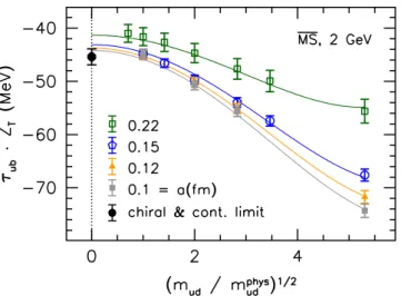
Notice that τf bdiverges fora→0 for any quark mass, except in the chiral limit, where it is ultraviolet-finite. This tendency is clearly visible in figure 6, which shows our results for the up quark. Therefore, we can define an ultraviolet-finite observable for the light quarks, without any zero-temperature subtraction, namely the chiral limit of the tensor coefficient. In contrast, to calculate χ^spin we will need to take differences between results obtained at different temperatures (see below).

The ansatz (2.9) contains the free parameters τ_f and µ_QED. In addition, we include a quadratic mass-dependence and lattice artifacts of O(a²) to each parameter in the fit.

Varying the fit ranges ina and inm_ud/m^phys_ud as well as the functional form, we carry out several acceptable fits that are used to build a histogram for the chiral continuum limit of

JHEP07(2020)183

Figure 6. Light quark mass-dependence of the tensor coefficient atT = 0 for the up quark using our four finest lattice spacings (green to gray symbols). The indexbindicates that the QED divergence that one encounters at mud > 0 has not been subtracted. The results diverge logarithmically towards the continuum limit for any mud 6= 0. In contrast, the chiral limit is free of ultraviolet divergences and a combined chiral and continuum limit exists (black circle).

the tensor coefficient. In this combined limit we obtain in the MS scheme T = 0 : f_γ^⊥(2 GeV)≡ lim

m_ud→0τ_ub·Z_T(2 GeV) =−45.4(1.5) MeV. (4.4) The central value differs from our previous result [26] f_γ^⊥ =−40.3(1.4) MeV, mainly due to the multiplicative renormalization factor that we determined non-perturbatively here, see figure 11 in appendix D.

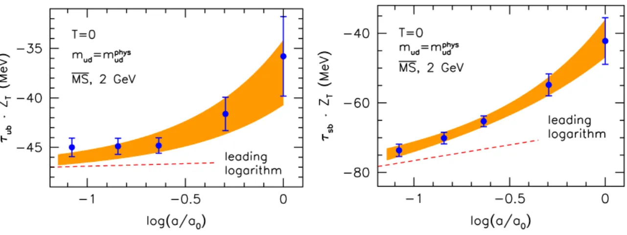
In the left panel of figure 7 we show thea-dependence of theT = 0 light quark tensor coefficientτ_ub·Z_T at the physical point and the result of the above interpolation, including the systematic error estimated using the different fits. For demonstration purposes, we also indicate the leading logarithmic behavior, that we obtain by subtracting the lattice artifact terms from the central fit. Comparing to the similar plot for χ_b (figure 3), we see that deviations from the continuum behavior are sizable (and are predominantly due to the fact that we are dealing with a dimensionful quantity in this case). For this reason, here we cannot reliably determine the value of µ_QED. Nevertheless, we note that fixing the renormalization scale to its value from eq. (4.2) also gives acceptable fits. This is in agreement with the expectation of section 2.3, as well as with the results in the free case, see appendix C.4. The logarithmic divergence ∝ m_floga becomes more pronounced for heavy quarks. This is visible in the right panel of figure7, where we plot the strange quark tensor coefficientτ_sb·Z_T atm_ud=m^phys_ud against the lattice spacing and again indicate the leading logarithmic term.

As we have discussed above, at non-vanishing values of the quark mass m_f, the tensor coefficient diverges logarithmically. In ref. [26] we suggested to cancel this by taking the

JHEP07(2020)183

Figure 7. The bare tensor coefficient for the up quark (left panel) and for the strange quark (right panel) at the physical point and at zero temperature (blue points), together with an interpolation (orange bands). For the up quark this interpolation is them_ud=m^phys_ud slice of a two-dimensional fit like in figure6. The red dashed lines indicate the leading logarithmic divergence∝mflogain both fits. The remaining a-dependence is consistent with lattice artifacts. We always use ms=m^phys_s . The lattice spacing is normalized toa0= 1.46 GeV⁻¹.

logarithmic derivative with respect to the quark mass, see also ref. [14]:

f_γf^⊥ =

1−m_f ∂

∂m_f

τ_f ·Z_T . (4.5)

This renormalization prescription will give identical results for any regulator, up to the multiplicative factor Z_T.¹² Using this prescription, it turns out thatf_γu^⊥ =f_γd^⊥ =f_γ^⊥ holds within statistical errors. For the strange quark we obtain:

f_γs^⊥ =−68(3)(4) MeV. (4.6) The first error includes the described variation of the fit while the second error reflects the uncertainty of the derivative with respect to ms that we indirectly determine from the dependence of the tensor coefficient on the light quark mass, following the procedure explained in ref. [26].

In the literature often the magnetic susceptibility of the quark condensate, X_u = τ_u

ψ¯uψu

·Z_T ZS

, (4.7)

is given, rather than f_γ^⊥ =τu·Z_T. Since the latter quantity has a smaller anomalous di- mension and its value does not depend on a separate computation of the chiral condensate, this is the preferred choice for practical applications. However, for convenience of com- parison, we shall convert it into the other convention. The numerical value of the quark condensate in the SU(2) chiral limit in the MS scheme at the scale µ_QCD = 2 GeV reads

12This construction will not only cancel the logarithmic divergence but also any finite term∝mf. Should this be unwanted then one will have to accept a scheme-dependence and convert between different schemes in a similar way as is done for the massive chiral condensate, e.g., in ref. [58].

JHEP07(2020)183

hψ¯_uψ_ui = [272(5) MeV]³ [59]. To enable a comparison with other results, below we also listXu at the scaleµQCD= 2 GeV. Since most literature values refer to a low, sometimes unspecified scale, in addition we run X_u as well asf_γ^⊥ to the scaleµ_QCD = 1 GeV, which is used in most sum rule calculations, see, e.g., refs. [16, 17, 19]. This is done, using the five-loop β- and quark mass anomalous dimension γ-functions [56,60] and the three-loop γ-function of the tensor current [36,61]. The results read

Xu(2 GeV) =−[665(13) MeV]⁻² , Xu(1 GeV) =−[542(11) MeV]⁻² , (4.8)

f_γ^⊥(1 GeV) =−51.1(1.6) MeV, (4.9)

where we have added all errors in quadrature, including the uncertainty off_γ^⊥(2 GeV), the difference between running with the two- and three-loop γ-functions of the tensor current, the uncertainty of hψ¯_uψ_ui and the uncertainty of the strong coupling parameter [57]. All the above results are in the MS-scheme.

We summarize earlier results from the literature for comparison. The first sum rule determination of X_u [14] suggested a value X_u(0.5 GeV) =−[350(50) MeV]⁻² while vector meson dominance yields [35] X_u ≈ 2/m_ρ ≈ −(540 MeV)⁻². This was improved upon in subsequent sum rule determinations, see, e.g., ref. [19] and references therein. The most extensive sum rule study [19] foundX_u(1 GeV)≈ −(560 MeV)⁻², which agrees reasonably well with our determination. A comparatively smaller absolute value f_γ^⊥ ≈ −38 MeV was obtained at a low scaleµ∼600 MeV in the quark-soliton model [18] while the Vainshtein relation [62] suggests an even smaller modulus of the magnetic susceptibility of the quark condensate Xu = −N_c/(4π²F_π²) ≈ −(335 MeV)⁻². This parameter was also considered in holographic studies, with the result Xu ≈ −(295 MeV)⁻² [63], while NJL- and quark- meson-model predictions give X_u ≈ −(480 MeV)⁻² [64] and X_u ≈ −(440 MeV)⁻² [64], respectively. Finally, quenched lattice simulations, without renormalization, gave the val- ues Xu ≈ −[804(3) MeV]⁻² in SU(2) gauge theory [65] and Xu ≈ −[486(21) MeV]⁻² in SU(3) [66]. Our previous full QCD study [26] resulted inX_u(2 GeV) =−[693(13) MeV]⁻², however, in that case the renormalization was only carried out perturbatively.

Our result (4.6) for the strange quark coefficient translates into

Xs(2 GeV) =−[565(50) MeV]⁻² , Xs(1 GeV) =−[460(41) MeV]⁻² , (4.10)

f_γs^⊥(1 GeV) =−76.5(5.7) MeV, (4.11)

where we used the ratiohψ¯_sψ_si/hψ¯_uψ_ui= 1.08(17) [58] for the conversion betweenf_γs^⊥ and Xs. The difference between Xs and Xu(1 GeV)≈ −(475 MeV)⁻² has been reported to be negligible in the sum rule calculations [17].

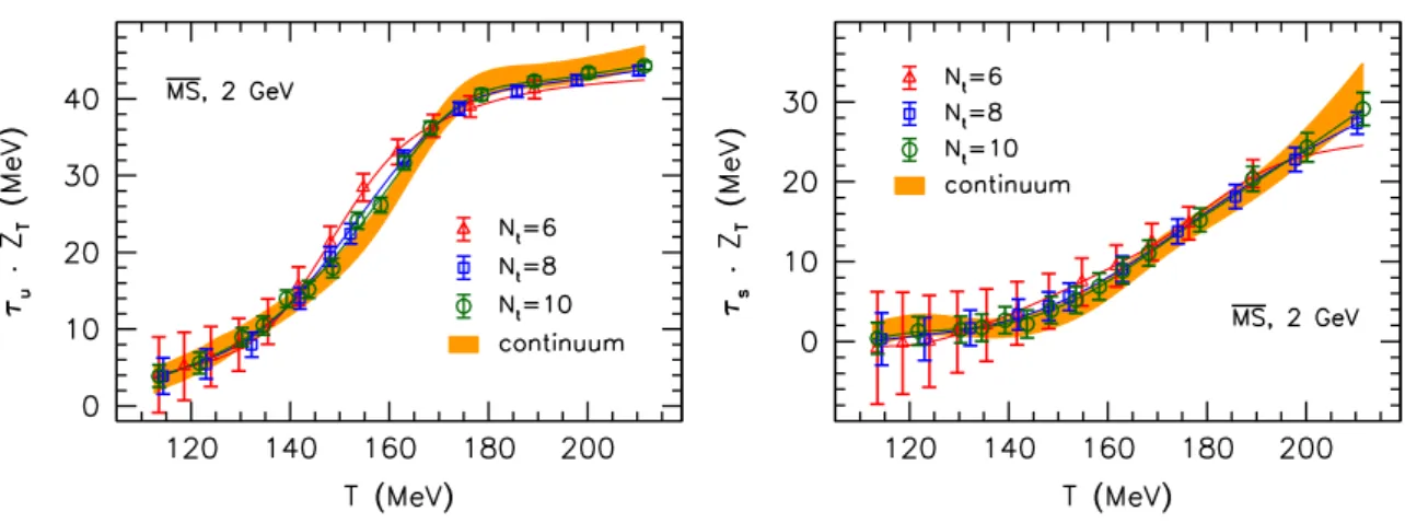
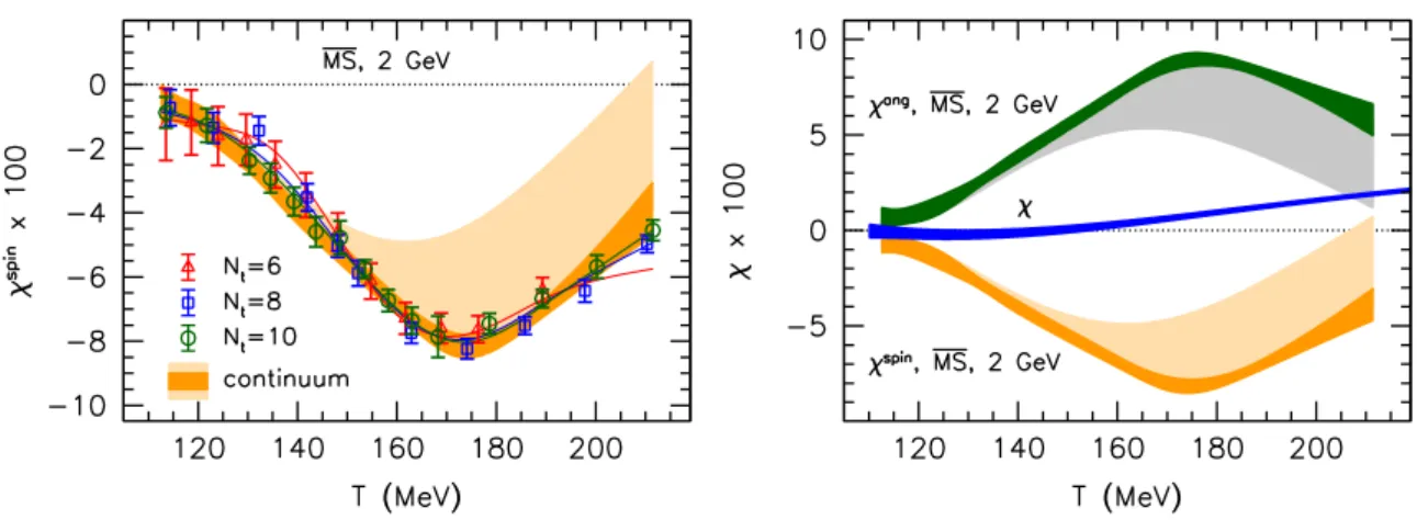
4.3 The spin contribution at T > 0

Having interpolated theT = 0 tensor coefficients, we are now in the position to perform the additive renormalization (2.10) by subtracting this contribution from the finite temperature results. We use our existing Nt = 6, 8 and 10 results from ref. [26] to approach the continuum limit. Especially in light of the slow convergence of χ towards a→ 0, see the right panel of figure 5, this extrapolation should be backed up with finer lattice ensembles