Light-cone distribution amplitudes of the baryon octet

JHEP02(2016)070

Published for SISSA by Springer

Received: December 10, 2015 Accepted: January 20, 2016 Published: February 10, 2016

Light-cone distribution amplitudes of the baryon octet

Gunnar S. Bali,^a,b Vladimir M. Braun,^a Meinulf G¨ockeler,^a Michael Gruber,^a Fabian Hutzler,^a Andreas Sch¨afer,^a Rainer W. Schiel,^a Jakob Simeth,^a Wolfgang S¨oldner,^a Andre Sternbeck^c and Philipp Wein^a

aInstitut f¨ur Theoretische Physik, Universit¨at Regensburg, Universit¨atsstraße 31, D-93040 Regensburg, Germany

bDepartment of Theoretical Physics, Tata Institute of Fundamental Research, Homi Bhabha Road, Mumbai 400005, India

cTheoretisch-Physikalisches Institut, Friedrich-Schiller-Universit¨at Jena, Max-Wien-Platz 1, D-07743 Jena, Germany

E-mail: michael1.gruber@physik.uni-regensburg.de, fabian.hutzler@physik.uni-regensburg.de,

philipp.wein@physik.uni-regensburg.de

Abstract: We present results of the first ab initio lattice QCD calculation of the nor- malization constants and first moments of the leading twist distribution amplitudes of the full baryon octet, corresponding to the small transverse distance limit of the associated S-wave light-cone wave functions. The P-wave (higher twist) normalization constants are evaluated as well. The calculation is done using Nf = 2 + 1 flavors of dynamical (clover) fermions on lattices of different volumes and pion masses down to 222 MeV. Significant SU(3) flavor symmetry violation effects in the shape of the distribution amplitudes are observed.

Keywords: Lattice QCD, Nonperturbative Effects ArXiv ePrint: 1512.02050

JHEP02(2016)070

Contents

1 Introduction 1

2 Baryon distribution amplitudes 4

2.1 Leading twist distribution amplitudes 5

2.2 Higher twist contributions 9

3 Lattice formulation 10

3.1 Correlation functions 10

3.1.1 Leading twist — zeroth moments 11

3.1.2 Leading twist — first moments 12

3.1.3 Higher twist 14

3.2 Details and strategy of the lattice simulation 14

4 Renormalization 17

5 Chiral extrapolation and SU(3) flavor breaking 19

6 Results 25

7 Conclusions and outlook 31

A The baryon octet 33

B Operator relations 36

B.1 Relation to H(4) operators 36

B.2 Operator bases for renormalization 37

C Renormalization procedure 38

1 Introduction

Understanding the structure of matter in terms of quark and gluon degrees of freedom is the ultimate goal of the physics of strong interactions. For this purpose, the intuitive quantum- mechanical representation of a hadron as a superposition of Fock states with different numbers of partons in the infinite momentum frame (or using light-cone quantization) is very useful in order to develop the underlying physics picture. It also provides a good basis for theoretical modeling. Although a priori there is no reason to expect that, e.g., the nucleon wave function components with, say, 100 partons (quarks and gluons) are suppressed relative to those with only three valence quarks, the phenomenological success of

JHEP02(2016)070

quark models suggests that in many cases only the first few Fock components are important.

Also the analysis of hard exclusive reactions involving large momentum transfer from the initial to the final state baryon within QCD perturbation theory [1–3] suggests that such processes are dominated by the overlap of the valence light-cone wave functions at small transverse separations, usually referred to as light-cone distribution amplitudes (DAs).

The DAs can be viewed as light-cone wave functions integrated over the quark trans- verse momenta [1]. They are fundamental nonperturbative functions that are complemen- tary to conventional parton distributions, but are more elusive because their relation to experimental observables is less direct compared to quark parton densities. DAs are scale- dependent and for asymptotically large scales they are given by simple expressions, the so-called asymptotic DAs [1,3]. There are many indications, however, that these asymp- totic expressions poorly approximate the real DAs for the range of momentum transfers accessible in present experiments.

The theoretical description of DAs is based on the relation of their moments, i.e., integrals over DAs weighted by powers of momentum fractions, to matrix elements of local operators. Such matrix elements can be estimated using nonperturbative techniques and the DAs can be reconstructed as an expansion in a suitable basis of polynomials in the momentum fractions.

First estimates of the first and the second moments of the baryon DAs have been obtained more than 30 years ago using QCD sum rules (QCDSR) [4–7]. These early calculations suggested large deviations from the corresponding asymptotic values and were used extensively for model building of DAs [4–8] that allowed for a reasonable description of the experimental data available at that time within a purely perturbative framework, see the review [3].

Despite its phenomenological success, this approach has remained controversial over the years. In particular the QCD sum rules used to calculate the moments have been criticized as unreliable, see, e.g., ref. [9]. Also, nowadays it is commonly accepted that perturbative contributions to hard exclusive reactions at accessible energy scales must be complemented by the so-called soft or end-point corrections. Estimates of the soft contributions using QCD sum rules [10], quark models [11] and light-cone sum rules [12–14] favor nucleon DAs that deviate only mildly from the asymptotic expressions.

It has now become possible to calculate moments of the DAs from first principles using lattice QCD. The first quantitative results for the nucleon have been obtained by the QCDSF collaboration [15, 16] using two flavors of dynamical (clover) fermions, followed by [17], where a much larger set of lattices was used including ensembles at smaller pion masses, close to the physical point. The latter paper also contained an exploratory study of the DAs of negative parity nucleon resonances, see also ref. [18].

In this work we extend the analysis of ref. [17] to the full J^P = ¹₂⁺ baryon octet.

In addition to theoretical completeness, our study is motivated by applications to weak decays of heavy baryons such as Λ_b and Λ_c. Such baryons are produced copiously at the LHC. As more data are collected, studies of rareb-baryon decays involving flavor-changing neutral currents offer interesting insights into the quark mixing matrix and, potentially, may reveal new physics beyond the Standard Model. In particular the Λ_b → Λµ⁺µ⁻

JHEP02(2016)070

decays are receiving a lot of attention, see, e.g., refs. [19, 20] and references therein. B- meson decays into baryon-antibaryon pairs are also interesting. The pattern of SU(3) flavor symmetry breaking in weak decays is known in general to be nontrivial. In particular the large asymmetry observed in the decay Σ⁺→pγ has been fueling a lot of discussions over many years and remains poorly understood at the parton level (see, e.g., ref. [21]). Another motivation comes from the emerging possibilities to study the transition form factors for the electroexcitation of nucleon resonances at large photon virtualities, planned for the JLAB 12 GeV upgrade [22], with the hope that similar transition form factors for hyperon production, e.g., in large-angle πN scattering, will also become accessible in the future.

This perspective already stimulated several theory studies, see, e.g., refs. [23,24].

In this first study we will mainly address the development of the necessary formalism and methodical issues. Studies of hyperon DAs have a long history [6], however, we found that the definitions existing in the literature are not very convenient to study effects of SU(3) breaking and that the standard notation is, in part, contradictory. Therefore, we explain our notation and provide the necessary definitions in the introductory section 2.

The physical interpretation of the DAs in terms of light-cone wave functions is considered as well. The related appendixA explains the phase conventions for the flavor wave functions used in this work.

Section 3 is devoted to the lattice formulation of the problem at hand, the definition of correlation functions used in our analysis of the couplings and the first moments of baryon octet DAs, and the strategy to approach the physical limit of small pion mass.

Calculations in this work are performed on a set of ensembles provided by the coordinated lattice simulations (CLS) effort [25]. These are obtained using the tree-level Symanzik improved gauge action and 2+1 dynamical Wilson (clover) quark flavors. In our calculation we start at the flavor symmetric point, where all quark masses are equal, and approach the real world in such a way that u and d quark masses decrease and simultaneously the squark mass increases so that the average mass is kept (approximately) constant [25,26].

Section 4, complemented by appendicesBand C, explains our renormalization proce- dure. We employ a nonperturbative method based on the well-known RI⁰/SMOM scheme, combined with matching factors calculated in continuum perturbation theory to convert our results to the MS scheme. The renormalization of flavor-octet operators turns out to be more complicated than the nucleon case and is discussed in some detail.

Section5contains a discussion of chiral extrapolation and SU(3) symmetry breaking in the framework of three-flavor baryon chiral perturbation theory (BChPT). Our presentation is based on the recent analysis in ref. [27]. One result is a simple relation between the DAs of the Σ and Ξ hyperons which has the same theory status as the famous Gell-Mann-Okubo sum rule for baryon masses and is satisfied to high accuracy for our lattice data.

In section 6 our final results are presented and compared with the existing lattice (for the nucleon) and QCD sum rule calculations. We find that deviations of the baryon DAs from their asymptotic form at hadronic scales are small, up to an order of magnitude smaller than in old QCD sum rule calculations. The SU(3) breaking in the corresponding shape parameters is, on the contrary, much larger than anticipated. Section 7 is reserved for a summary and conclusions.

JHEP02(2016)070

It has to be said that while our calculation provides the first qualitative insight into SU(3) breaking of octet baryon DAs from lattice QCD, it has not yet reached a quantita- tively mature state. This is mainly due to the lack of a continuum extrapolation, which can have a significant impact on DAs (cf. ref. [17]). Actually, the whole CLS strategy to simulate with open boundary conditions is motivated by the fact that, at presently used lattice constants, discretization errors are significant. Moreover, on coarse lattices the lat- tice spacing will depend on the observable employed for scale setting. As our study is an exploratory one with significant systematic uncertainties, this fact is irrelevant in the present context. We use ensembles with the lattice spacing a = 0.0857(15) fm, which is determined from the Wilson flow method as described in ref. [25]. The dimensionless flow timet0/a² was extrapolated to the physical point and the lattice spacing was then assigned by matching to the continuum limit value√

t₀= 0.1465(21)(13) fm determined in ref. [28].

In the future we intend to include finer lattices, which are currently being generated within the CLS effort. This will then allow us to take the continuum limit and also eliminate scale setting ambiguities related to the nonzero lattice spacing.

2 Baryon distribution amplitudes

Baryon DAs [1–3] are defined as matrix elements of renormalized three-quark operators at light-like separations:

B^{f gh}_αβγ(a1, a2, a3;µ) =h0|

fα(a1n)gβ(a2n)hγ(a3n)MS

|B(p, λ)i, (2.1) where|B(p, λ)iis the baryon state with momentumpand helicityλ, whileα, β, γare Dirac indices,nis a light-cone vector (n²= 0), the a_i are real numbers,µis the renormalization scale and f, g, h are quark fields of the given flavor, chosen to match the valence quark content of the baryon B. The Wilson lines, which are needed for gauge invariance, as well as the color antisymmetrization, which is needed to form a color singlet, are not written out explicitly but always implied. Renormalization of three-quark operators using dimensional regularization and minimal subtraction requires some care; we will be using the renormalization scheme proposed in ref. [29].

Restricting ourselves to the analysis of the lowest ¹₂⁺multiplet, neglecting electromag- netic interactions and assuming exact isospin symmetry (ml ≡ mu =md), it is sufficient to consider four cases:

B ∈ {N ≡p,Σ≡Σ⁻,Ξ≡Ξ⁰,Λ}. (2.2) For definiteness we choose the following flavor ordering:

p: (f, g, h) = (u, u, d), (2.3a)

Σ⁻ : (f, g, h) = (d, d, s), (2.3b)

Ξ⁰ : (f, g, h) = (s, s, u), (2.3c)

Λ : (f, g, h) = (u, d, s), (2.3d)

JHEP02(2016)070

respectively. This choice is always implied so that in what follows we do not show flavor indices. Matrix elements for other baryons and/or with different flavor ordering can be obtained in a straightforward manner using isospin transformations.

The general Lorentz decomposition of the matrix element (2.1) consists of 24 terms [30]

that are usually written in the form B_αβγ(a₁, a₂, a₃;µ) =X

DA

Γ^DA

αβ Γ˜^DAu^B(p, λ)

γ

Z

[dx]e^−ip·nP

iaixi DA^B(x₁, x₂, x₃;µ). (2.4) Here Γ^DA and ˜Γ^DA are the Dirac structures corresponding to the distribution amplitude DA^B(x_i), see eq. (2.9) of ref. [30], andu^B(p, λ) is the Dirac spinor with on-shell momentum p (p² = m²_B) and helicity λ. This decomposition can be organized in such a way that all DAs have definite collinear twist. The scale dependence will be suppressed from now on, unless it is explicitly needed. The variablesx1, x2, x3 are the momentum fractions carried by the quarks f, g, h, respectively, and the integration measure is defined as

Z [dx] =

1

Z

0 1

Z

0 1

Z

0

dx1dx2dx3δ(1−x1−x2−x3). (2.5)

The factor δ(1−x₁−x₂−x₃) enforces momentum conservation.

2.1 Leading twist distribution amplitudes

In this work we will mainly be concerned with the DAs of leading twist three. To this accuracy the general decomposition in eq. (2.4) is simplified to three terms [3]:

4B_αβγ(a1, a2, a3) = Z

[dx]e^−ip·nP

iaixi (2.6)

×

v_αβ;γ^B V^B(x1, x2, x3)+a^B_αβ;γA^B(x1, x2, x3)+t^B_αβ;γT^B(x1, x2, x3)+. . .

.

Here

v^B_αβ;γ = (˜nC)/ _αβ(γ₅u^B₊(p, λ))_γ, (2.7a) a^B_αβ;γ = (˜nγ/ ₅C)_αβ(u^B₊(p, λ))_γ, (2.7b) t^B_αβ;γ = (iσ⊥˜nC)_αβ(γ^⊥γ5u^B₊(p, λ))γ, (2.7c) with the charge conjugation matrix C and the notation

˜

nµ=pµ−1 2

m²_B

p·nnµ, u^B₊(p, λ) = 1 2

˜ / n/n

˜

n·nu^B(p, λ), (2.8a) σ⊥˜n⊗γ^⊥=σ^µρn˜_ρg^⊥_µν⊗γ^ν, g^⊥_µν =g_µν−n˜µnν+ ˜nνnµ

˜

n·n . (2.8b)

Our DAs V^N,A^N and T^N correspond to V₁,A₁ and T₁ in ref. [30].

JHEP02(2016)070

The equivalent definition in terms of the right- and left-handed components of the quark fields, q^↑(↓)= ¹₂(1±γ5)q, is sometimes more convenient:

h0| f^↑T(a₁n)C /ng^↓(a₂n)

nh/ ^↑(a₃n)|B(p, λ)i=

=−1

2(p·n)/nu^B↑(p, λ) Z

[dx]e^−ip·nP

iaixi [V −A]^B(x₁, x₂, x₃), (2.9a) h0| f^↑T(a₁n)Cγ^µ/ng^↑(a₂n)

γ_µnh/ ^↓(a₃n)|B(p, λ)i=

= 2(p·n)/nu^B↑(p, λ) Z

[dx]e^−ip·nP

iaixi T^B(x1, x2, x3), (2.9b) where u^B↑(p, λ) = ¹₂(1+γ5)u^B(p, λ). In the nucleon case the combination [V −A]^N appearing in the first of these equations is traditionally referred to as the leading twist nucleon DA Φ^N. For the full octet we define

Φ^B6=Λ(x₁, x₂, x₃) = [V −A]^B(x₁, x₂, x₃), (2.10a) Φ^Λ(x₁, x₂, x₃) =−

r2 3

[V −A]^Λ(x₁, x₂, x₃)−2[V −A]^Λ(x₃, x₂, x₁) . (2.10b) If Φ^B is given, the V^B and A^B components can be reconstructed due to their different symmetry properties under the exchange of the first and the second quark:

V^B6=Λ(x₂, x₁, x₃) = +V^B(x₁, x₂, x₃), V^Λ(x₂, x₁, x₃) =−V^Λ(x₁, x₂, x₃), (2.11a) A^B6=Λ(x2, x1, x3) =−A^B(x1, x2, x3), A^Λ(x2, x1, x3) = +A^Λ(x1, x2, x3), (2.11b) T^B6=Λ(x2, x1, x3) = +T^B(x1, x2, x3), T^Λ(x2, x1, x3) =−T^Λ(x1, x2, x3). (2.11c) Using isospin symmetry one can further show for the nucleon

T^N(x₁, x₃, x₂) = 1 2

Φ^N(x₁, x₂, x₃) + Φ^N(x₃, x₂, x₁)

, (2.12)

so that, to leading twist accuracy, Φ^N contains all necessary information. For other baryons this relation does not hold, so that the functions T^B are independent of [V −A]^B.

To fully exploit the benefits of SU(3) flavor symmetry it proves convenient to define the following set of DAs:

Φ^B6=Λ_± (x1, x2, x3) = 1 2

[V −A]^B(x1, x2, x3)±[V −A]^B(x3, x2, x1) , (2.13a) Π^B6=Λ(x1, x2, x3) =T^B(x1, x3, x2), (2.13b)

Φ^Λ₊(x₁, x₂, x₃) = r1

6

[V −A]^Λ(x₁, x₂, x₃) + [V −A]^Λ(x₃, x₂, x₁) , (2.13c) Φ^Λ₋(x₁, x₂, x₃) =−

r3 2

[V −A]^Λ(x₁, x₂, x₃)−[V −A]^Λ(x₃, x₂, x₁) , (2.13d) Π^Λ(x1, x2, x3) =√

6T^Λ(x1, x3, x2), (2.13e)

where for the nucleon Π^N = Φ^N₊ up to isospin breaking effects. In the limit of SU(3) flavor symmetry, where m_u = m_d = m_s (and in particular at the flavor symmetric point with

JHEP02(2016)070

physical average quark mass indicated by ?), the following relations hold:¹

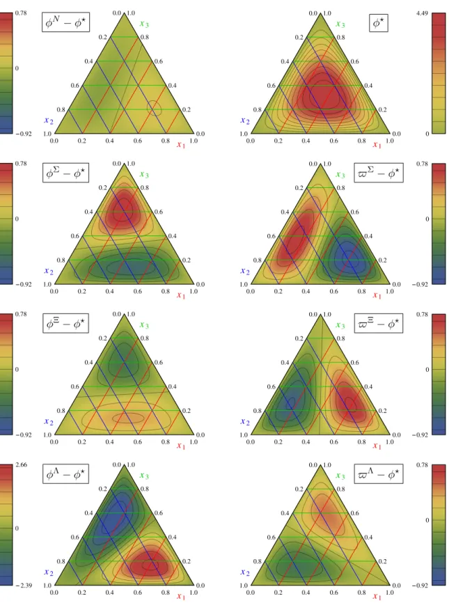
Φ^?₊≡Φ^{N ?}₊ = Φ^Σ?₊ = Φ^Ξ?₊ = Φ^Λ?₊ = Π^{N ?}= Π^Σ? = Π^Ξ?, (2.14a) Φ^?₋≡Φ^{N ?}₋ = Φ^Σ?₋ = Φ^Ξ?₋ = Φ^Λ?₋ = Π^Λ?. (2.14b) Therefore, the amplitudes Π^B (or T^B) only need to be considered when flavor symmetry is broken. In the flavor symmetric limit Φ^?₊ and Φ^?₋ can again be combined to form a single distribution amplitude Φ^? = Φ^?₊+ Φ^?₋. One can show (see the detailed discussion in section 5) that to first order in the symmetry breaking parameter, m²_K−m²_π ∝ms−ml, the following relation holds:

Φ^Σ₊−Π^Σ = Π^Ξ−Φ^Ξ₊. (2.15)

To understand the physical meaning of the DAs it is instructive to work out their relation to light-front wave functions. The leading twist approximation corresponds to taking into account S-wave contributions in which case the helicities of the quarks sum up to the helicity of the baryon (cf. refs. [31, 32]). Suppressing the transverse momentum dependence one finds

|(B 6= Λ)^↑i=

Z [dx]

8√

6x₁x₂x₃|f ghi ⊗

[V +A]^B(x₁, x₂, x₃)|↓↑↑i+ [V −A]^B(x₁, x₂, x₃)|↑↓↑i

−2T^B(x₁, x₂, x₃)|↑↑↓i

=

Z [dx]

8√

3x₁x₂x₃|↑↑↓i ⊗

−√

3Φ^B₊(x₁, x₃, x₂) |MS, Bi −√

2|S, Bi /3

−√

3Π^B(x₁, x₃, x₂) 2|MS, Bi+√

2|S, Bi /3 +Φ^B₋(x1, x3, x2)|MA, Bi ,

(2.16)

and

|Λ^↑i=

Z [dx]

4√

6x1x2x3

|udsi ⊗

[V +A]^Λ(x1, x2, x3)|↓↑↑i+[V−A]^Λ(x1, x2, x3)|↑↓↑i

−2T^Λ(x1, x2, x3)|↑↑↓i

=

Z [dx]

8√

3x₁x₂x₃|↑↑↓i ⊗

−√

3Φ^Λ₊(x1, x3, x2)|MS,Λi +Π^Λ(x1, x3, x2) 2|MA,Λi+

√

2|A,Λi /3 +Φ^Λ₋(x₁, x₃, x₂) |MA,Λi −√

2|A,Λi /3 ,

(2.17)

where|↑↓↑i etc. show quark helicities and |f ghi stands for the flavor ordering as specified in eq. (2.3). |MS, Biand|MA, Biare the usual mixed-symmetric and mixed-antisymmetric octet flavor wave functions, respectively (see tables 9 and 10 of appendix A). |A,Λi and

|S, B 6= Λi are totally antisymmetric and symmetric flavor wave functions (see tables 8 and11), which only occur in the octet if SU(3) symmetry is broken. From this representa- tion it becomes obvious that V^B,A^B and T^B are convenient DAs if one sorts the quarks with respect to their flavor, while Φ^B₊, Φ^B₋ and Π^Bcorrespond to three distinct flavor struc- tures in a helicity-ordered wave function. At the flavor symmetric point Φ^?₊and Φ^?₋isolate

1Our phase conventions for the baryon states and the corresponding flavor wave functions are detailed in appendixA.

JHEP02(2016)070

the mixed-symmetric and mixed-antisymmetric flavor wave functions:

|B^↑i^? =

Z [dx]

8√

3x₁x₂x₃|↑↑↓i ⊗

−√

3Φ^?₊(x1, x3, x2)|MS, Bi+ Φ^?₋(x1, x3, x2)|MA, Bi . (2.18) DAs can be expanded in a set of orthogonal polynomials (conformal partial wave expansion) in such a way that the coefficients have autonomous scale dependence at one loop. The first few polynomials are (see, e.g., ref. [33])

P₀₀= 1, P₂₀= 63

10[3(x₁−x₃)²−3x₂(x₁+x₃) + 2x²₂], (2.19a) P₁₀= 21(x1−x3), P₂₁= 63

2 (x1−3x2+x3)(x1−x3), (2.19b) P₁₁= 7(x1−2x2+x3), P₂₂= 9

5[x²₁+ 9x2(x1+x3)−12x1x3−6x²₂+x²₃]. (2.19c) Note that all P_nk have definite symmetry (being symmetric or antisymmetric) under the exchange of x₁ and x₃. Taking into account the corresponding symmetry of the DAs, defined in eq. (2.13), a generic expansion reads

Φ^B₊= 120x₁x₂x₃ ϕ^B₀₀P₀₀+ϕ^B₁₁P₁₁+ϕ^B₂₀P₂₀+ϕ^B₂₂P₂₂+. . .

, (2.20a)

Φ^B₋= 120x₁x₂x₃ ϕ^B₁₀P₁₀+ϕ^B₂₁P₂₁+. . .

, (2.20b)

Π^B6=Λ= 120x1x2x3 π₀₀^BP₀₀+π^B₁₁P₁₁+π₂₀^BP₂₀+π₂₂^BP₂₂+. . .

, (2.20c)

Π^Λ= 120x1x2x3 π₁₀^ΛP₁₀+π^Λ₂₁P₂₁+. . .

. (2.20d)

In this way all nonperturbative information is encoded in the set of (scale-dependent) coefficients ϕ^B_nk, π_nk^B, which can be related to matrix elements of local operators. In each DA only polynomials of one type, either symmetric or antisymmetric under exchange ofx₁ and x₃, appear.

The leading contributions 120x1x2x3ϕ^B₀₀ and 120x1x2x3π₀₀^B6=Λ are usually referred to as the asymptotic DAs. The corresponding normalization coefficients ϕ^B₀₀ and π^B6=Λ₀₀ can be thought of as the wave functions at the origin (in position space). In what follows we will use the notation

f^B=ϕ^B₀₀, f_T^B6=Λ=π₀₀^B. (2.21) Note that for the nucleon the two couplings coincide, f_T^N = f^N. For the Λ baryon the zeroth moment of T^Λ vanishes. The higher-order coefficients are usually referred to as shape parameters. Note that, in contrast to ref. [17], we do not separate the couplingsf^B and f_T^B6=Λ as overall normalization factors, so that our ϕ^N_nk correspond to f_Nϕ^N_nk of [17].

The one-loop scale evolution of the couplings and shape parameters is given by ϕ^B_nk(µ) =ϕ^B_nk(µ0)

α_s(µ) αs(µ0)

γnk/β0

, π_nk^B(µ) =π_nk^B(µ0)

α_s(µ) αs(µ0)

γnk/β0

, (2.22) where β₀ = 11−2N_f/3 is the first coefficient of the QCD β-function. In this work we restrict ourselves to the contributions of first order polynomials P₁₀, P₁₁ and omit all higher terms. The relevant one-loop anomalous dimensions are

γ₀₀= 2

3, γ₁₁= 10

3 , γ₁₀= 26

9 . (2.23)

JHEP02(2016)070

The scale dependence of f^B and f_T^B6=Λ is identical and is known up to three-loop order, see refs. [29,34].

2.2 Higher twist contributions

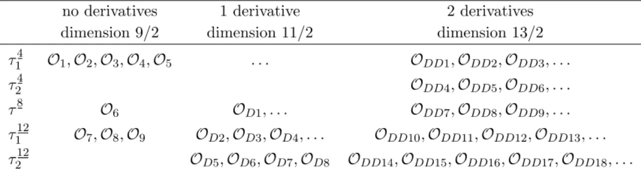
The general decomposition (2.4) contains 21 DAs of higher twist, which altogether involve only up to three new normalization constants (just two for N, Σ and Ξ), for details see refs. [27,30]. They can be defined as matrix elements of local three-quark twist four op- erators without derivatives. These twist four couplings are also interesting in a broader context, e.g., in studies of baryon decays in generic GUT models [35], and as input param- eters for QCD sum rule calculations, see, e.g., refs. [24,36,37].

We use the following definitions:

h0| f^↑T(0)Cγ^µg^↓(0)

γ_µh^↑(0)|(B 6= Λ)(p, λ)i=−1

2λ^B₁m_Bu^B↓(p, λ), (2.24a) h0| f^↑T(0)Cσ^µνg^↑(0)

σ_µνh^↑(0)|(B 6= Λ)(p, λ)i=λ^B₂m_Bu^B↑(p, λ), (2.24b) for the isospin-nonsinglet baryons (N, Σ, Ξ) and

h0| u^↑T(0)Cγ^µd^↓(0)

γ_µs^↑(0)|Λ(p, λ)i= 1 2√

6λ^Λ₁m_Λu^Λ↓(p, λ), (2.25a) h0| u^↑T(0)Cd^↑(0)

s^↓(0)|Λ(p, λ)i= 1 2√

6λ^Λ_Tm_Λu^Λ↓(p, λ), (2.25b) h0| u^↑T(0)Cd^↑(0)

s^↑(0)|Λ(p, λ)i= −1 4√

6λ^Λ₂m_Λu^Λ↑(p, λ), (2.25c) for the Λ baryon. The definitions are chosen such that at the flavor symmetric point

λ^?₁≡λ^{N ?}₁ =λ^Σ?₁ =λ^Ξ?₁ =λ^Λ?₁ =λ^Λ?_T , (2.26a) λ^?₂≡λ^{N ?}₂ =λ^Σ?₂ =λ^Ξ?₂ =λ^Λ?₂ , (2.26b) cf. ref. [27]. For the nucleon the definitions in terms of chiral fields in eq. (2.24) are equivalent to the traditional definitions of λ^N₁ and λ^N₂ not involving chiral projections, as used in ref. [17]. Analogous definitions can also be given for the Λ baryon:

h0| u^T(0)Cγ^µγ₅d(0)

γ_µs(0)|Λ(p, λ)i= −1

√6λ^Λ₁m_Λu^Λ(p, λ), (2.27a) h0| u^T(0)Cd(0)

γ₅s(0)|Λ(p, λ)i= −1 4√

6(λ^Λ₂ + 2λ^Λ_T)m_Λu^Λ(p, λ), (2.27b) h0| u^T(0)Cγ5d(0)

s(0)|Λ(p, λ)i= −1 4√

6(λ^Λ₂ −2λ^Λ_T)mΛu^Λ(p, λ). (2.27c) The one-loop evolution for all twist four normalization constants is the same:

λ^B_1,2,T(µ) =λ^B_1,2,T(µ₀)

α_s(µ) αs(µ0)

−2/β0

. (2.28)

The corresponding anomalous dimensions are known up to three-loop accuracy [29, 34].

The scale dependence of the couplingsλ^B₁ andλ^Λ_T is the same to all orders, whereas forλ^B₂ it differs starting from the second loop.

JHEP02(2016)070

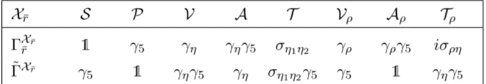
X_¯r S P V A T V_ρ A_ρ T_ρ

Γ^X_r¯^r¯ 1 γ₅ γ_η γ_ηγ₅ σ_η1η2 γ_ρ γ_ργ₅ iσ_ρη Γ˜^Xr¯ γ₅ 1 γ_ηγ₅ γ_η σ_η1η2γ₅ γ₅ 1 γ_ηγ₅

Table 1. Definition of the Dirac matrix structures that appear in the local operators which are used in the lattice calculation, see eq. (3.2). Lorentz indices appearing in both Γ^X_r¯^¯r and ˜Γ^Xr¯ are summed over implicitly.

3 Lattice formulation

In Euclidean spacetime a direct calculation of DAs is not possible, since this would require quark fields at light-like separations. However, lattice QCD allows us to access moments of the DAs, e.g.,

V_lmn^B = Z

[dx]x^l₁x^m₂ xⁿ₃V^B(x1, x2, x3), (3.1) and similarly for the other functions. They are related to matrix elements of local three- quark operators, whose general form reads

X^B,lmn

¯

r¯lm¯¯n =^ijk

i^lD¯lf^T(0)i

CΓ^X_r¯^r¯

i^mD_m¯g(0)j Γ˜^Xr¯

iⁿD_¯nh(0)k

. (3.2)

Here we use a multi-index notation for the covariant derivatives, D¯l ≡ D_λ1· · ·D_λl. The Dirac structures that we consider, Γ^X_r¯^r¯ and ˜Γ^X¯r, are listed in table 1.² As sources for the baryon fields we have used the interpolating currents

N^N = u^TCγ5d

u , (3.3a)

N^Σ = d^TCγ5s

d , (3.3b)

N^Ξ = s^TCγ5u

s , (3.3c)

N^Λ= 1

√6 2 u^TCγ5d

s+ u^TCγ5s

d+ s^TCγ5d u

, (3.3d)

with an optimized number of smearing steps in the quark sources to suppress excited state contributions. The other baryons can then be obtained by means of isospin symmetry.

3.1 Correlation functions

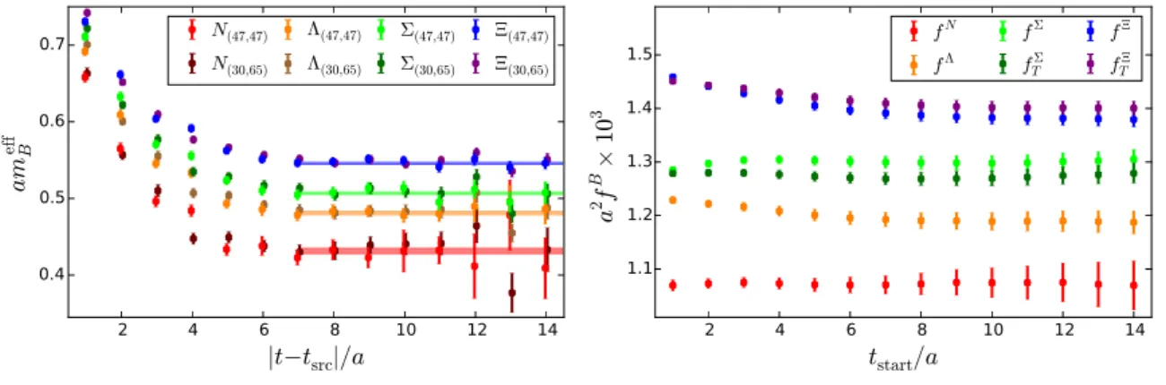
Moments of baryon DAs can be extracted from the ground state contribution to the two- point correlation functions. Neglecting the exponentially suppressed excited states the correlation functions can be written as

hO_τ(t,p) ¯N_τ^B0(0,p)i=

√Z_B

2E_B X

λ

h0|O_τ(0)|B(p, λ)iu¯^B_τ0(p, λ)e^−EBt, (3.4) with the energy E_B =E_B(p) = p

m²_B+p², where we assume the continuum dispersion relation. The momentum-dependent coupling Z_B =Z_B(p) describes the overlap between

2Starting from this section all equations refer to Euclidean spacetime; we use the gamma matrix con- vention of [16].

JHEP02(2016)070

the smeared source operator and the physical baryon ground state and can be obtained from the correlator

hN_τ^B(t,p) ¯N_τ^B0(0,p)(γ₊)_τ⁰_τi=Z_Bm_B+kE_B

E_B e^−EBt, (3.5)

where γ₊ = (1+kγ₄)/2 with k = m_B^∗/E_B^∗ suppresses the negative parity contribu- tion [17,38].³

3.1.1 Leading twist — zeroth moments

In order to extract the leading twist normalization constants, the following linear combi- nations of operators are constructed such that their matrix elements do not contain any contributions of higher twist:

O^B,000_X,A =−γ₁X₁^B,000+γ₂X₂^B,000, (3.6a) O^B,000_X,B =−γ₃X₃^B,000+γ₄X₄^B,000, (3.6b) O^B,000_X,C =−γ₁X₁^B,000−γ2X₂^B,000+γ3X₃^B,000+γ4X₄^B,000, (3.6c) where X can be V, A orT. The leading twist baryon couplings can be determined from the following correlation functions:

C_X^B,000_,A =h γ₄O^B,000_X,A (t,p)

τN¯_τ^B0(0,p)(γ₊)_τ⁰_τi

=c_XX₀₀₀^B p

Z_Bk(p²₁−p²₂) EB

e^−EBt,

(3.7a) C_X^B,000_,B =h γ₄O^B,000_X,B (t,p)

τN¯_τ^B0(0,p)(γ₊)_τ⁰_τi

=cXX₀₀₀^B p ZB

EB(mB+kEB) +kp²₃ EB

e^−EBt,

(3.7b) C_X^B,000_,C =h γ₄O^B,000_X,C (t,p)

τN¯_τ^B0(0,p)(γ₊)_τ⁰_τi

=cXX₀₀₀^B p ZB

EB(mB+kEB) +k(p²₁+p²₂−p²₃)

E_B e^−EBt,

(3.7c)

wherecV =cA= 1 andcT =−2. Again,X can beV,AorT. In practice we only consider the zero momentum correlatorsC_X,B^B,000 andC_X^B,000_,C as they are less noisy and, therefore, can be measured with higher accuracy. The couplings of interest are related to the calculated zeroth moments as follows:

f^B6=Λ≡ϕ^B₀₀=V₀₀₀^B , f^Λ ≡ϕ^Λ₀₀=− r2

3A^Λ₀₀₀, f_T^B6=Λ≡π₀₀^B =T₀₀₀^B , (3.8) where f_T^N = f^N due to isospin symmetry. The remaining zeroth moments of the leading twist DAs V^B,A^B andT^B vanish:

V₀₀₀^Λ =A^B6=Λ₀₀₀ =T₀₀₀^Λ = 0. (3.9)

3B^∗denotes the negative parity partner of the baryonB.

JHEP02(2016)070

3.1.2 Leading twist — first moments

First moments of DAs can be calculated utilizing operators containing one covariant deriva- tive. For l+m+n= 1 we define the leading twist combinations

O^B,lmn_X,A = +γ₁γ₃X_{13}^B,lmn+γ₁γ₄X_{14}^B,lmn−γ₂γ₃X_{23}^B,lmn−γ₂γ₄X_{24}^B,lmn−2γ₁γ₂X_{12}^B,lmn, (3.10a) O^B,lmn_X,B = +γ₁γ₃X_{13}^B,lmn−γ₁γ₄X_{14}^B,lmn+γ₂γ₃X_{23}^B,lmn−γ₂γ₄X_{24}^B,lmn+2γ₃γ₄X_{34}^B,lmn, (3.10b) O^B,lmn_X,C =−γ₁γ₃X_{13}^B,lmn+γ₁γ₄X_{14}^B,lmn+γ₂γ₃X_{23}^B,lmn−γ₂γ₄X_{24}^B,lmn, (3.10c) where the braces indicate symmetrization. For the calculation of the first moments of the leading twist DAs one can use the correlation functions (l+m+n= 1)

C_X,A,1^B,lmn=h γ₄γ₁O^B,lmn_X,A (t,p)

τN¯_τ^B0(0,p)(γ₊)_τ⁰_τi

=−c_XX_lmn^B p ZBp1

EB(mB+kEB) +k(2p²₂−p²₃) EB

e^−EBt,

(3.11a) C_X,A,2^B,lmn=h γ4γ2O^B,lmn_X,A (t,p)

τN¯_τ^B0(0,p)(γ+)τ⁰τi

= +c_XX_lmn^B p Z_Bp2

EB(mB+kEB) +k(2p²₁−p²₃)

E_B e^−EBt,

(3.11b) C_X,A,3^B,lmn=h γ4γ3O^B,lmn_X,A (t,p)

τN¯_τ^B0(0,p)(γ+)_τ⁰_τi

=−c_XX_lmn^B p

Z_Bp₃k(p²₁−p²₂)

E_B e^−EBt,

(3.11c)

C_X,B,1^B,lmn=h γ4γ1O^B,lmn_X,B (t,p)

τN¯_τ^B0(0,p)(γ+)τ⁰τi

= +cXX_lmn^B p ZBp1

EB(mB+kEB) +kp²₃

E_B e^−EBt,

(3.11d) C_X,B,2^B,lmn=h γ4γ2O^B,lmn_X,B (t,p)

τN¯_τ^B0(0,p)(γ+)_τ⁰_τi

= +c_XX_lmn^B p

Z_Bp₂E_B(m_B+kE_B) +kp²₃

E_B e^−EBt,

(3.11e) C_X,B,3^B,lmn=h γ₄γ₃O^B,lmn_X,B (t,p)

τN¯_τ^B0(0,p)(γ₊)_τ⁰_τi

=−c_XX_lmn^B p

Z_Bp₃2E_B(m_B+kE_B) +k(p²₁+p²₂) EB

e^−EBt,

(3.11f)

C_X,C,1^B,lmn=h γ4γ1O^B,lmn_X,C (t,p)

τN¯_τ^B0(0,p)(γ+)_τ⁰_τi

=−c_XX_lmn^B p

Z_Bp₁E_B(m_B+kE_B) +kp²₃

E_B e^−EBt,

(3.11g) C_X,C,2^B,lmn=h γ₄γ₂O^B,lmn_X,C (t,p)

τN¯_τ^B0(0,p)(γ₊)_τ⁰_τi

= +c_XX_lmn^B p

Z_Bp₂E_B(m_B+kE_B) +kp²₃ EB

e^−EBt,

(3.11h) C_X,C,3^B,lmn=h γ₄γ₃O^B,lmn_X,C (t,p)

τN¯_τ^B0(0,p)(γ₊)_τ⁰_τi

= +cXX_lmn^B p ZBp3

k(p²₁−p²₂) EB

e^−EBt.

(3.11i)

JHEP02(2016)070

One immediately notices that at least one nonzero component of spatial momentum is required to extract the first moments. We evaluate C_X^B,lmn_,A,1 ,C_X^B,lmn_,B,1 and C_X^B,lmn_,C,1 with mo- mentum in xdirection (p= (±1,0,0)),⁴ andC_X^B,lmn_,A,2 ,C_X^B,lmn_,B,2 andC_X^B,lmn_,C,2 with momentum in y direction (p = (0,±1,0)). For momentum in z direction (p = (0,0,±1)) only the correlator C_X,B,3^B,lmn can be used. We do not consider the remaining two correlators as they require a higher number of nonvanishing momentum components, which would lead to larger statistical uncertainties.

The shape parameters defined in eq. (2.20) can be expressed as linear combinations of V_lmn^B ,A^B_lmn andT_lmn^B via eq. (2.13). For the N, Σ and Ξ baryons,

ϕ^B6=Λ₁₁ = 1

2 [V −A]^B₁₀₀−2[V −A]^B₀₁₀+ [V −A]^B₀₀₁

, (3.12a)

ϕ^B6=Λ₁₀ = 1

2 [V −A]^B₁₀₀−[V −A]^B₀₀₁

, (3.12b)

π^B6=Λ₁₁ = 1

2 T₁₀₀^B +T₀₁₀^B −2T₀₀₁^B

, (3.12c)

whereπ^N₁₁=ϕ^N₁₁ due to isospin symmetry. For the Λ baryon, ϕ^Λ₁₁= 1

√6 [V −A]^Λ₁₀₀−2[V −A]^Λ₀₁₀+ [V −A]^Λ₀₀₁

, (3.13a)

ϕ^Λ₁₀=− r3

2 [V −A]^Λ₁₀₀−[V −A]^Λ₀₀₁

, (3.13b)

π^Λ₁₀= r3

2 T₁₀₀^Λ −T₀₁₀^Λ

. (3.13c)

In addition we define combinations corresponding to the sum of contributions with the derivative acting on each of the three quarks:

ϕ^B6=Λ_00,(1)= [V −A]^B₁₀₀+ [V −A]^B₀₁₀+ [V −A]^B₀₀₁, (3.14a) π^B6=Λ_00,(1)=T₁₀₀^B +T₀₁₀^B +T₀₀₁^B , (3.14b) ϕ^Λ_00,(1)=

r2

3 [V −A]^Λ₁₀₀+ [V −A]^Λ₀₁₀+ [V −A]^Λ₀₀₁

, (3.14c)

where π^N_00,(1) = ϕ^N_00,(1) due to isospin symmetry. Thanks to the Leibniz product rule for derivatives, this sum can be written as a total derivative acting on a local three-quark operator without derivatives so that in the continuum

ϕ^B_00,(1)=ϕ^B₀₀, π^B6=Λ_00,(1) =π₀₀^B, (3.15) corresponding to the momentum conservation condition x1+x2+x3 = 1, see eq. (2.5).

However, the Leibniz rule is violated by lattice discretization and this relation can only be expected to hold after continuum extrapolation in a renormalization scheme which respects the Lorentz symmetry. Note that under renormalization ϕ^B_00,(1) and π_00,(1)^B6=Λ mix with the other first moments, see section4. It turns out that for the bare lattice values the

4All momentum components are given as multiples of 2π/L(Lbeing the spatial extent of the lattice).

JHEP02(2016)070

equalities (3.15) are violated significantly. After renormalization and conversion to the MS scheme we find that the sum rules (3.15) are fulfilled to an accuracy between ≈96% and

≈98% for our value of the lattice spacing a≈0.0857 fm, see tables 4 and 5. A violation of the momentum sum rule of this size is in perfect agreement with the results in ref. [17], where similar discretization effects have been observed.

3.1.3 Higher twist

Higher twist normalization constants can be calculated from the correlation functions hX_τ^B,000(t,p) ¯N_τ^B0(0,p)(γ+)_τ⁰_τi=κ^B_XmB

pZB

mB+kEB

E_B e^−EBt, (3.16) where X can be S, P, V, A or T, cf. eq. (3.2) and table 1. The twist four couplings of interest defined in eqs. (2.24) and (2.25) are given by

λ^B6=Λ₁ =−κ^B_V, λ^B6=Λ₂ =κ^B_T , (3.17a)

λ^Λ₁ =−√

6κ^Λ_A, λ^Λ₂ =−2√

6 κ^Λ_S+κ^Λ_P

, λ^Λ_T =−√

6 κ^Λ_S−κ^Λ_P

. (3.17b) Due to symmetry properties of the associated operators it follows that

κ^B6=Λ_S =κ^B6=Λ_P =κ^Λ_V =κ^B6=Λ_A =κ^Λ_T = 0, (3.18) and the corresponding correlators vanish.

3.2 Details and strategy of the lattice simulation

In this analysis we use lattice ensembles generated within the coordinated lattice simula- tions (CLS) effort. These N_f = 2 + 1 simulations employ the nonperturbatively order a improved Wilson (clover) quark action and the tree-level Symanzik improved gauge action.

We used a modified version of the Chroma software system [39,40], the LibHadronAnalysis library and efficient inverters [41–43]. To enhance the ground state overlap the source inter- polators are Wuppertal-smeared [44], employing spatially APE-smeared [45] transporters.

A special feature of CLS configurations is the use of open boundary conditions in time direction [43, 46]. This will eventually allow for simulations at very fine lattices without topological freezing. We achieve an efficient and stable hybrid Monte Carlo (HMC) sam- pling by applying twisted-mass determinant reweighting [43], which avoids near-zero modes of the Wilson Dirac operator.

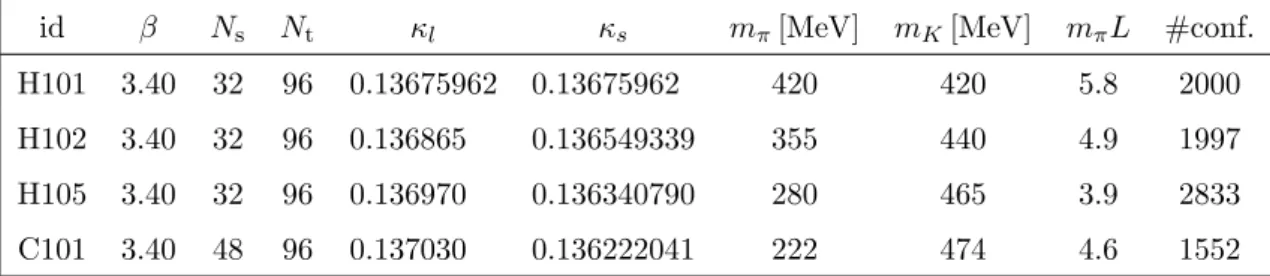
A list of the CLS ensembles used in this work is given in table2. As schematically rep- resented in figure1, these ensembles are tuned such that the average quark mass reproduces (approximately) the physical value. They have rather large spatial volumes (L > 2.7 fm,

with mπL & 4) and high statistics. Consecutive gauge field configurations are separated

by four molecular dynamics units.

Lattice calculations with the average quark mass fixed at the physical value have already been carried out for hadron masses and some form factors [26, 47, 48]. At the flavor symmetric point hadrons form SU(3) multiplets and their properties are related by symmetry. For example the masses have to be equal for all octet baryons. The real world is then approached in such a way thatu and dquark masses decrease and simultaneously thesquark mass increases so that their average is kept constant.