Hadroquarkonium from lattice QCD

(1)

Hadroquarkonium from lattice QCD

Maurizio Alberti,¹Gunnar S. Bali,^2,3Sara Collins,² Francesco Knechtli,¹ Graham Moir,⁴ and Wolfgang Söldner²

1Department of Physics, Bergische Universität Wuppertal, Gaußstraße 20, 42119 Wuppertal, Germany

2Institut für Theoretische Physik, Universität Regensburg, Universitätsstraße 31, 93053 Regensburg, Germany

3Department of Theoretical Physics, Tata Institute of Fundamental Research, Homi Bhabha Road, Mumbai 400005, India

4Department of Applied Mathematics and Theoretical Physics, Centre for Mathematical Sciences, University of Cambridge, Wilberforce Road, Cambridge CB3 0WA, United Kingdom (Received 24 August 2016; revised manuscript received 27 February 2017; published 3 April 2017)

The hadroquarkonium picture [S. Dubynskiy and M. B. Voloshin, Phys. Lett. B 666, 344 (2008)]

provides one possible interpretation for the pentaquark candidates with hidden charm, recently reported by the LHCb Collaboration, as well as for some of the charmoniumlike“X,Y,Z”states. In this picture, a heavy quarkonium core resides within a light hadron giving rise to four- or five-quark/antiquark bound states. We test this scenario in the heavy quark limit by investigating the modification of the potential between a static quark-antiquark pair induced by the presence of a hadron. Our lattice QCD simulations are performed on a Coordinated Lattice Simulations (CLS) ensemble with Nf¼2þ1 flavors of nonperturbatively improved Wilson quarks at a pion mass of about 223 MeV and a lattice spacing of about a¼0.0854fm. We study the static potential in the presence of a variety of light mesons as well as of octet and decuplet baryons. In all these cases, the resulting configurations are favored energetically. The associated binding energies between the quarkonium in the heavy quark limit and the light hadron are found to be smaller than a few MeV, similar in strength to deuterium binding. It needs to be seen if the small attraction survives in the infinite volume limit and supports bound states or resonances.

DOI:10.1103/PhysRevD.95.074501

I. INTRODUCTION

Recently, the LHCb Collaboration found two structures in the decay Λb→J=ψpK, which can be interpreted as candidates for pentaquark states with hidden charm, containing three light quarks, in addition to a charm quark-antiquark pair[1,2]. The most likely spin and parity assignments for these candidates, labeled P^þ_cð4380Þ and P^þ_cð4450Þ, are J^P ¼3=2⁻ and 5=2^þ, respectively, with 3=2^þand5=2⁻being another possibility. While the nature of these (and of some other structures) is still disputed[3,4], the number of established charmonium resonances certainly has exploded during the past 15 years, see Ref.[5]and, e.g., Ref.[6]for a more recent review. Many of these are of an exotic nature and some clearly hint at light quark-antiquark or—in the case of theP_ccandidates—even atqqqcompo- nents, in addition to the charm quark and antiquark.

Many models can accommodate some, or if extended to include states that contain five (anti-)quarks, even all of these resonances: tetraquarks [7–9] consisting of diquark-antidiquark pairs, including a recently proposed

“dynamic”picture[10,11], molecules of two open charm mesons[12–16], hybrid states[17–20]containing a charm quark-antiquark pair and additional valence gluons, hadro- charmonium with a compact charmonium core bound inside a light hadron [21,22], and mixtures of the above.

Here we will specifically aim to establish if the last picture (hadroquarkonium) is supported in the heavy quark limit.

The standard way of addressing a strongly decaying resonance and extracting the position of the associated pole in the unphysical Riemann sheet from simulations in Euclidean spacetime boxes was introduced by Lüscher [23]. For applications of this and related methods to charmonium spectroscopy, see, e.g., Ref. [24] and refer- ences therein. In the case of charmonia, this is particularly challenging since, in addition to ground states, radial excitations need to be considered and the number of different decay channels can be large, some with more than two hadrons in the final state. Moreover, while in principle resonance parameters can be computed, at least below inelastic multiparticle thresholds, these will not necessarily tell us much about the“nature”of the under- lying state: how does the naive quark model need to be modified to provide a guiding principle for the existence or nonexistence of an exotic resonance?

A direct computation of the scattering parameters of, e.g., a nucleon-charmonium resonance in a realistic setting constitutes a serious computational challenge, especially if one aims at conclusive results with meaningful errors.

Instead of directly approaching the problem at hand, here we restrict ourselves to the heavy quark limit in which the charm quarks can be considered as slowly moving in the background of gluons, sea quarks and, possibly, light hadrons.

After integrating out the degrees of freedom associated with the heavy quark massm_Q, quarkonia can be described

(2)

in terms of an effective field theory: nonrelativistic QCD (NRQCD) [25]. In the limit of small distances r, or equivalently, large momentum transfers m_Qv, where v is the interquark velocity, the scale m_Qv∼1=r can also be integrated out, resulting in potential NRQCD (pNRQCD) [26,27]. Then, to leading order in r with respect to the pNRQCD multipole expansion and to v²∼αs in the NRQCD power counting, quarkonium becomes equivalent to a nonrelativistic quantum mechanical system, where the interaction potential is given by the static potential V₀ðrÞ which can, e.g., be computed nonperturbatively from Wilson loop expectation valueshWðr; tÞiin Euclidean spacetime,

V₀ðrÞ ¼−lim

t→∞

d

dtlnhWðr; tÞi: ð1Þ Here we investigate whether this potential becomes modified in the presence of a light hadron. This would then lower or increase quarkonium energy levels. If embedding the quarkonium in the light hadron is energetically favorable, this would suggest a bound state, at least for sufficiently large quark masses.

This article is organized as follows. In Sec.IIwe briefly discuss previous studies of nucleon-charmonium bound states and comment on the ordering of scales that we consider. In Sec. III we define the observables that we compute. Then, in Sec. IV we describe details of the simulation, before numerical results are presented in Sec.V.

Subsequently, in Sec.VIwe relate the modifications of the static potential to quarkonium bound state energies, before we summarize in Sec. VII.

II. NUCLEON-CHARMONIUM BOUND STATES Light meson exchanges between a single nucleon or nucleons bound in a nucleus and quarkonium, which does not contain any light valence quarks, are suppressed by the Zweig rule. Therefore, such interactions should be dominated by gluon exchanges. In the heavy quark limit, quarkonium can be considered essentially as a point particle of a heavy quark and antiquark bound by the short-range perturbative Coulomb potential. The first nonvanishing chromodynamical multipole is then a dipole and quarkonium may interact with the nuclear environment via color dipole-dipole van der Waals forces. For a recent discussion of the relevant scales in the context of effective field theories, see Ref. [28]. Initially, using phenomenological interaction potentials, nucleon-charmonium binding energies ranging from 20 MeV[29,30] down to 10 MeV[31]

were estimated for nuclei consisting ofA >3[29,31]and A >10[30]nucleons. A first QCD-based estimate[32]for the potential between quarkonium in the heavy quark limit and a nucleus resulted inϒandJ=ψ binding energies of a few MeV and 10 MeV, respectively, possibly with large relativistic and higher-order multipole corrections in the charmonium case. This discussion of light nuclei hosting a

quarkonium state may have contributed to the suggestion of quarkonium states that are embedded within light hadrons, hadroquarkonia[22].

At present no (p)NRQCD lattice studies of baryon- charmonium states exist. However, a few investigations employing relativistic charm quarks have been carried out.

In Ref.[33], theηcandJ=ψcharmonia were scattered with light pseudoscalar and vector mesons as well as with the nucleon, in the quenched approximation with rather large light quark mass values; the ratioM_π=m_ρranged from 0.9 down to 0.68. Varying the lattice extent fromL¼1.6fm over 2.2 fm up to 3.2 fm, in this pioneering work scattering lengths were extracted, indicating some attraction in all the channels investigated. A similar study was performed in Ref.[34], combining staggered sea with domain wall light and Fermilab charm quarks; however, unusually small scattering lengths were reported. Finally, a pseudoscalar charm quark-antiquark pair was created along with a nucleon and even with light nuclei by the NPLQCD Collaboration [35]. In this work the binding energy reported for the nucleon case was about 20 MeV, albeit at a rather large light quark mass value, corresponding to M_π≈800 MeV, and for a coarse lattice spacinga≈0.145 fm. This value of the binding energy is consistent with some of the expectations for charmonia in a nuclear environment discussed above.

Closest in spirit to the van der Waals interaction picture, Kawanai and Sasaki [36] in a quenched study, again at rather large pion masses, M_π≥640MeV, computed a charmonium-nucleon Bethe-Salpeter wave function.

Plugging this into a Schrödinger equation, a potential between the charmonium and the nucleon was extracted, indicating very weak attractive forces.

Here we will not assume a nonrelativistic light hadron of massm_H, whose dipole-dipole interaction with quarkonium can be described by a potential. Instead, our light hadron is an extended relativistic object. We also go beyond the point- dipole approximation in the heavy quark sector by“pulling” quark and antiquark apart by a distancer. We then determine the modification of the interaction potential between the heavy quark-antiquark pair, that we approximate as static sources, induced by the presence of a light hadron. To be more precise, we will consider the limit m_Q≫m_H, m_Q≫ΛQCD, whereΛQCDdenotes a typical nonperturbative scale of a few hundred MeV, andv²≪1. Since we determine the quark-antiquark potential, i.e., the matching function between NRQCD and pNRQCD, nonperturbatively,m_Qv∼ 1=rdoes not need to be much larger thanΛQCD. However, we neglect color octet contributions[26,27], which may become significant at distancesr≳Λ⁻¹QCD.

III. STATIC POTENTIALS “INSIDE” HADRONS We denote an interpolator creating a static fundamental color chargeQat a positionzþr=2and destroying it at a positionz−r=2asQ^†rðzÞ. This will transform according to

MAURIZIO ALBERTIet al. PHYSICAL REVIEW D 95,074501 (2017)

(3)

the fundamental 3 representation of the gauge group atzþ r=2and according to3atz−r=2and hence it contains a gauge covariant transporter connecting these two points (usually a spatially smeared Schwinger line). The Wilson loop can then be written as

hWðr; tÞi ¼ h0jQrT^t=aQ^†rj0i; ð2Þ where we assume rotational invariance is restored for r¼ jrj≫a, and T ¼e^−aH denotes the transfer matrix connecting adjacent time slices.

Within the static approximation, there are different strategies to investigate bound states containing a heavy quark-antiquark pair and additional light quarks. One method, which we are not going to pursue here, amounts to creating a light hadron H containing either qq¯ or qqq along with the stringy QQ¯ state at equal Euclidean time.

The interpolator for creating a zero-momentum projected tetra- or pentaquark state then has the form

Pr¼X

z

HðzÞQ^†rðzÞ: ð3Þ

Note that the creation interpolatorHof a hadronic state (as well asPr) will carry a spinor index, which we suppress.

The correlator of interest is now h0jPrT^t=aPrj0i. Even without summing over positions z this is automatically projected onto zero momentum at source and sink as the light hadron is tied in position space to the static quarks, see Eq.(3). Numerous possibilities exist for where to spatially place the light quarks relative to the heavy sources within the interpolator Pr and how to transport and contract the color such that the interpolator respects the correct gauge transformation properties. This freedom can be exploited to enhance the overlap of Prj0i with the physical state and may also provide some insight into its internal structure.

Subsequent to a pioneering lattice study[37] of a light qq pair bound in the above way to two static antitriplet sources, quite a few simulations of a lightqq¯ pair bound to the string state created by Q^†r have also been carried out.

Such results exist both for a light quark-antiquark pair with isospin I¼1 [38–41] and I¼0 [39,42]. In contrast, a static quark-antiquark pair accompanied by three light quarks has not been investigated on the lattice so far.

Instead of creating tetra- or pentaquark states containing a heavy or static quark and the corresponding antiquark, here we wish to “directly” address a particular picture of such bound states, hadroquarkonium[21,22]. This will be achieved by computing differences between the static potential in the presence of a light hadron, relative to the static potential in the vacuum. The former can be obtained from the large Euclidean time decay of

hHjQrT^t=aQ^†rjHi; ð4Þ

wherejHiis the ground state that is destroyed by the zero- momentum interpolator

H≡X

x

HðxÞ: ð5Þ

In order to evaluate the expectation value Eq. (4) we create a hadronic state at time 0. We then let it propagate to δt to achieve ground-state dominance. At this time we create an additional quark-antiquark string by inserting a (smeared) Wilson loop of time extentt, which terminates at tþδt. Finally, we destroy the light hadron at the time tþ2δt. Then

hHjQrT^t=aQ^†rjHi∝ lim

δt→∞

h0jHT^δt=aQrT^t=aQ^†rT^δt=aHj0i h0jHT^{ðtþ2δtÞ=a}Hj0i ;

ð6Þ where we average over all spatial Wilson loop positionsz and light hadronic sink positions x. Zero-momentum projection at the light hadronic source can be avoided, due to the translational invariance of expectation values.

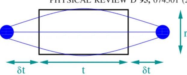
The correlator of interest is depicted in Fig.1.

We can now define the potential in the background of the hadron as

V_HðrÞ ¼−lim

t→∞

d

dtlnhHjQrT^t=aQ^†rjHi; ð7Þ in analogy to Eqs.(1)and(2). In the end we will compute differences

ΔV_HðrÞ ¼V_HðrÞ−V₀ðrÞ

¼−lim

t→∞

d

dtlnhHjQrT^t=aQ^†rjHi h0jQrT^t=aQ^†rj0i

¼−lim

t→∞

d

dtln hWðr; tÞC_H;2ptðtþ2δtÞi

hWðr; tÞihC_H;2ptðtþ2δtÞi; ð8Þ where the argument of the logarithm is simply the correlator of a light hadronic two-point function with the Wilson loop inserted, divided by the Wilson loop expectation value

t

δ

t

δ

t

r

FIG. 1. Graphical representation of the four-point correlation function in the numerator of Eq.(6)for the example of a static quark-antiquark pair at a distancerembedded in a baryon. Thin blue lines correspond to light quark propagators and the black rectangle to the Wilson loop.

(4)

times the hadronic two-point functionhC_H;2ptðtþ2δtÞi ¼ h0jHT^{ðtþ2δtÞ=a}Hj0i, see the denominator of Eq. (6).

We are now in the position to address the question within what hadronic channels ΔV_HðrÞ will be attractive and in what cases repulsive. This may serve as an indicator for the stability of related hadroquarkonia. In view of the recent LHCb result [1,2] baryonic states jHi are particularly interesting. For instance, adding the mass of theΔto that of the J=ψ gives 4329 MeV [43], which is not far away from the mass of the P_cð4380Þ. Furthermore, J^P¼3=2^þ can couple to1⁻to give3=2⁻. Another example is the sum of the nucleon (N) and χc2 masses, 4496 MeV, which is close to the mass of theP^þ_cð4450Þ. Again,1=2^þand2^þcan couple to J^P¼5=2^þ.

IV. IMPLEMENTATION AND TECHNICAL DETAILS

We analyse the N_f¼2þ1 ensemble “C101”, which has a volume of96×48³sites and was generated by the Coordinated Lattice Simulations (CLS) effort [44] using the openQCD simulation program [45,46]. Open boundary conditions in time and nonperturbatively order-a-improved Wilson fermions on top of the tree-level Symanzik improved Wilson gauge action are employed, see Ref.[44]for details on the simulation. To determine the lattice spacing we extrapolate the scale parametert₀[47]to the physical point, where we obtain ffiffiffiffiffiffi

8t₀

p =a¼4.852ð7Þ[48]. Using the continuum limit result ffiffiffiffiffiffi

8t₀

p ¼0.4144ð59Þð37Þfm [49]gives a¼0.0854ð15Þ fm. The pion and kaon masses on this ensemble areM_π≈223MeV andM_K≈476MeV, respectively. Note that while the pion is heavier than in nature the kaon is somewhat lighter since the sum of quark masses 2m_lþm_s(m_l¼m_u¼m_d) was adjusted to a value close to the physical one and kept constant within the main set of CLS simulations [44]. The spatial lattice extent reads L≈4.6=M_π≈4.1fm. For details see Ref.[48].

We analyse 1552 configurations, separated by four molecular dynamic units. On each of these configurations we place hadronic sources on 12 different time slices (30;43;44;…;52;53;65) at random spatial positions to reduce autocorrelations. Due to the use of open boundary conditions, we have to discard the boundary regions from our analysis. After carefully checking for translational invariance in time, we use forward and backward propa- gating hadronic two-point functions for the 11 sources¹ placed in the central region of the lattice but propagate only forward fromt₀=a¼30and backward fromðt−t₀Þ=a¼65.

This gives a total of24×1552two-point functions for each light hadron and spin polarization considered. Sinceδtneeds to be kept small to obtain statistically meaningful results, the quark propagators entering these two-point functions are

Wuppertal smeared at source and sink, using spatially smeared gauge transporters, to improve the overlap with the physical ground states.

We measure the Wilson loops using the publicly avail- ableWLOOPpackage[50], following the method described in Ref.[51]. In a first step, all gauge links are smeared using a single iteration of hypercubic (HYP) blocking [52].

Smearing the temporal links corresponds to a particular discretization choice of the static action and results in an exponential improvement of the signal-to-noise ratio of correlators involving static quarks[53]; HYP links reduce the coefficient of the divergent contribution to the self- energy of a static quark [39,54–56]. In a second step we construct a variational basis of Wilson loops using four different levels (0,5,7,12) of HYP smearing restricted to the three space dimensions.

To enable the construction of the correlators [Eq.(8)], we separately average the Wilson loops for each direction ofr, pointing along one of the three spatial lattice axes, and for different temporal positions. As detailed above, due to the use of open boundary conditions, our hadronic two-point functionsC_H;₂_ptðtÞare confined to the central time region of the lattice. We checked that ratios of Wilson loop expectation values, averaged over different temporal domains, centered about the middle of the lattice, were statistically consistent with 1. Furthermore, Eq.(8)was evaluated in two ways, restricting the Wilson loop average in the denominator to the same time slices as the averaging performed within the numerator as well as averaging the Wilson loop expectation value in the denominator within the whole region where boundary effects were negligible, from time slice 24 to 72.

The two results obtained for each quantity were statistically compatible with each other and below we will make use of the larger averaging region as this resulted in slightly smaller statistical errors.

For the error analysis, we apply the standard method of Ref. [57]. We include the reweighting factors due to twisted-mass reweighting and the rational approximation for the strange quark, see Ref. [46]. We checked that carrying out a more conservative analysis, estimating the effect of slow modes[58], only affects the errors in very few cases and never by more than 30%.

The distance r between the static sources breaks the continuum Oð3Þ symmetry down to the cylindrical sub- group Oð2Þ⊗Z₂¼D_∞h. Regarding fermionic represen- tations, i.e., for baryons, the double cover is reduced accordingly. In our implementation the static source-anti- source distanceris kept parallel to lattice axes. This means that the 48 element octahedral crystallographic group with reflectionsO_h is reduced to its 16 element subgroupD_4h (and its double cover O⁰_h to Dih₄⊗Dih₁). Therefore, when correlating hadrons with a continuum spin assign- ment J≥1 with the string state in the Σ^þg irreducible representation (irrep) ofD_∞h (A_1g of D_4h on the lattice), care has to be taken to construct the adequate irrep of the

1On time slice 47 two different spatial source positions were used.

(5)

cylindrical group. Below we address the continuum sit- uation but we have checked that the same arguments hold regarding the lattice irreps that we use. In the case of vector mesons, for example, theϕmeson, the1⁻ Oð3Þirrep will split into Πu and Σ^þu, the latter also appearing in the pseudoscalar channel. To block out this undesired contribution, we need to correlate a Wilson loop withrpointing in the z direction with the vector state destroyed by a polarized interpolator ðϕxþiϕyÞ= ffiffiffi

p2

. We average over cyclic permutations of x, y, and z. The decuplet baryon interpolator we use, for example for theΔbaryon, gives a state maximally polarized in thezdirection. This then has to be correlated with a Wilson loop pointing in the z direction too, to guarantee Λ¼ jJ_zj ¼3=2 and to avoid mixing with spin-1=2baryonic states. In this case we only used one polarization and therefore we cannot exploit averaging over different directions.

V. NUMERICAL RESULTS

Our strategy for testing the hadroquarkonium picture is to determine the potential between two static quarks in the vacuum and to compare this with its counterpart in the presence of a hadron. An energetically favorable difference may signal a tendency of the system to bind. In Sec.VAwe discuss the quality of our light hadronic effective masses and in Sec.V Bwe determine the potential in the vacuum, before moving on to Sec. V C where we investigate the modifications induced by the presence of hadrons.

We delay the discussion of the phenomenological conse- quences to Sec.VI.

A. Light hadronic effective masses

In the determination ofΔV_HðrÞbelow we will quote the δt¼δt_opt ¼5a≈0.43fm estimates as our final results.

With thisδtvalue, the fit intto the right-hand side of Eq.(8) is dominated by data with t≤t_max¼10a. Therefore, the hadronic effective masses

m_H;effðtþa=2Þ≡a⁻¹ln C_H;2ptðtÞ

C_H;2ptðtþaÞ ð9Þ should ideally exhibit plateaus for t≪t_maxþ2δt_opt¼ 20a≈1.7fm. We wish to check whether this is the case within the given statistics and for the quark smearing that we employ.

In Fig. 2 we display effective masses for some repre- sentative hadrons, namely theK, the nucleonN, and the cascades Ξ and Ξ, together with one-exponential fits to the plateau region. This region was determined from the requirement that the contribution of the second exponent of a two-exponential fit to data starting att¼3aamounted to less than 25% of the error of the correlation function. Using this criterion, indeed, in almost all the cases the plateau starts at t <10a¼2δt_opt¼ ðt_maxþ2δt_optÞ=2. One of the

few exceptions, that may very well be due to a statistical fluctuation, is theΞshown in the figure. We conclude that the ground-state overlap achieved for the light hadrons is sufficient for our purposes.

B. The static potential in the vacuum

As described in Sec. IV, we determine the static potential, V₀ðrÞ, from a variational procedure applied to a matrix of correlation functions consisting of spatially smeared Wilson loops. In Fig. 3, we show the physical quantity,V₀ðrÞ−V₀ð ffiffiffiffiffiffi

8t₀

p Þ, where the subtraction ensures that the self-energies of the static quarks are removed. The value of V₀ðrÞ at r¼ ffiffiffiffiffiffi

8t₀

p was obtained from a local interpolation, cf. Ref.[59]. For later use we also performed a fit to the Cornell parametrization[60]

V₀ðrÞ ¼μ−c

rþσr; ð10Þ FIG. 2. Effective masses Eq. (9), extracted from various hadronic two-point functions, together with results from one- exponential fits (shaded regions).

0 0.2 0.4 0.6 0.8 1 1.2

−800

−600

−400

−200 0 200 400 600 800 1000

FIG. 3. The quantityV₀ðrÞ−V₀ð ffiffiffiffiffiffi 8t₀

p Þ, whereV₀ðrÞ denotes the static quark-antiquark potential in the vacuum, together with the Cornell fit Eq.(10).

(6)

where μ denotes a constant offset (that diverges in the continuum limit),σis the string tension, and the Coulomb coefficient reads c¼4αs=3 at tree level. The fit with the parameter values,

μ¼0.721ð14ÞGeV; c¼0.468ð14Þ;

σ¼0.906ð16ÞGeV=fm; ð11Þ where we useda¼0.0854fm, is also shown in the figure.

To ensure that our results are not tainted by the breaking of the“string”between the static quarks, we only consider the static potential up to ∼1.2fm≈14a, the distance for which string breaking is expected to occur [39,61].

At larger distances, the phenomenological parametrization Eq. (10) is no longer valid and additional interpolating operators would be required to extract the true ground state. From the static potential, we compute the static force F¼V⁰ðrÞ and determine the Sommer scale [62], r₀≈0.5fm, from the equation r²FðrÞj_r¼r₀ ¼1.65, obtainingr₀=a¼5.890ð41Þ. We determiner₀from a local interpolation of the static force as it is explained in [51].

Indeed, at our lattice spacing and quark mass values,r₀≈5.89a≈5.89×0.0854fm≈0.50fm.

C. The static potential within a hadron

We now determine how the presence of a hadron alters the static potential. As discussed in Sec.III, we compute correlation functions

C_Hðr;δt; tÞ ¼ hWðr; tÞC_H;₂_ptðtþ2δtÞi

hWðr; tÞihC_H;2ptðtþ2δtÞi; ð12Þ where we average over the spatial Wilson loop and hadronic sink positions, for different hadronsH. For sufficiently large values oftand for fixed values ofrandδt, we can extract the difference between the static potential in the presence of the hadron,V_Hðr;δtÞ^δt→∞→ V_HðrÞ, and the vacuum static potential,V₀ðrÞ, from the exponential decay of this function in Euclidean time,

ΔV_Hðr;δtÞ≡V_Hðr;δtÞ−V₀ðrÞ

¼−lim

t→∞

d

dtln½CHðr;δt; tÞ: ð13Þ As the clover term that appears within the fermionic action extends one unit in time and we have also applied one level of four-dimensional HYP smearing to the Wilson loop, we only consider δt≥2a. In practice, we obtain statistically meaningful results forδt≲8a, and in some channels even larger values are possible. Note that within Eq. (12) no variational optimization is performed but we restrict ourselves to our highest level of 12 spatial HYP smearing iterations for the Wilson loops.

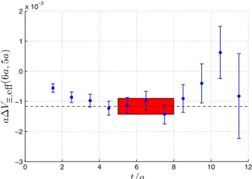
For a given hadron and for each combination ofrandδt, we perform linear fits in t to ln½Cðt;δt; tÞ within the effective energy plateau range. For examples see Figs. 4 and5, where we display effective energies for the cascade and the nucleon, respectively, for r¼6a≈0.51fm and δt¼5a, together with the results of the corresponding fits.

The errors are determined following Ref.[57]. Below we will assign an additional systematic error to our results from varying the fit range.

We will approximateΔV_HðrÞbyΔV_Hðr;δt¼5aÞ. The functional form is well described by the Cornell parametrization

ΔV_HðrÞ ¼ΔμH−Δc_H

r þΔσHr: ð14Þ The errors on the fit parametersΔμH,Δc_H, andΔσHwhich we will quote below will be indicative, since they only take

0 2 4 6 8 10 12

−3

−2

−1 0 1 2x 10⁻³

FIG. 4. Effective energy forΔV_Ξðr¼6a;δt¼5aÞ, defined in Eqs. (12) and (13), as a function of t. For the definition of effective energies, see Eq.(9). The error band shows our estimate forΔVðr;δtÞ, obtained from a linear fit to lnCHðr;δt; tÞ.

0 2 4 6 8 10

−5

−4

−3

−2

−1 0 1 2 3x 10⁻³

FIG. 5. The same as in Fig.4for the nucleon.

(7)

into account the statistical errors ofΔV_H and neglect their correlations. Below we summarize our results for the hadron H being a pseudoscalar or vector meson, a positive-parity octet or decuplet baryon, and a negative- parity baryon, respectively.

Note that theρandKmesons as well as the negative- parity baryons are not stable for our light quark mass value and lattice volume. However, using only quark-antiquark and three-quark interpolators, we are unable to detect their decays into pairs of p-wave pions, pion plus kaon, and s-wave pion plus positive-parity baryon, respectively. As we see effective energy plateaus, we also quote results for these channels. Clearly, this needs to be digested with some caution. We also note that the disconnected quark line contribution was neglected for theϕ meson.

1. Mesons

Several hidden charm resonances such as the Yð4260Þ have been interpreted as tightly bound quarkonium states, embedded within light mesonic matter [21,22]. Here we follow the procedure described above to calculate the modification of the static potential,ΔV_Hðr;δtÞ, for several light mesons.

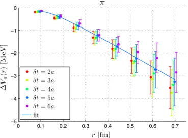
In Figs.6,7, 8, and9, we show our determinations for theπ,K,K^⋆, andϕmesons, respectively, where the color coding corresponds to different values of δt which are displaced horizontally in the plots for clarity.

In all the cases we findΔV_Hðr;δtÞ<0. When consid- ering the dependence on the spatial distance between the static sources, we observe a similar pattern for all the mesons; the modification of the static potential becomes more pronounced toward large distancesr. For distances up to about 0.3 fm, we generally findjΔV_Hðr;δtÞj≲1 MeV,

0 0.1 0.2 0.3 0.4 0.5 0.6 0.7

−5

−4

−3

−2

−1 0

FIG. 6. The modification to the static potential in the presence of a pion,ΔV_πðr;δtÞ. The color coding corresponds to different values ofδtas indicated in the legend, where the leftmost point within a group corresponds toδt¼2a. The curve shown is the result of a fit of theδt¼5adata to Eq.(14).

0 0.1 0.2 0.3 0.4 0.5 0.6 0.7

−5

−4

−3

−2

−1 0

FIG. 7. The same as in Fig. 6for the kaon.

0 0.1 0.2 0.3 0.4 0.5 0.6 0.7

−5

−4

−3

−2

−1 0

FIG. 8. The same as in Fig.6for theK^⋆ meson.

0 0.1 0.2 0.3 0.4 0.5 0.6 0.7

−5

−4

−3

−2

−1 0

FIG. 9. The same as in Fig.6for theϕmeson.

(8)

and at our largest shown distance of about 0.7 fm, we always findjΔV_Hðr;δtÞj≲4MeV. The values ofΔV_HðrÞ should be determined from the extrapolation δt→∞. In practice we find that all results for δt≳3a agree. The numbers obtained for δt¼5a represent a compromise between a value ofδtas large as possible and a reasonable signal-to-noise ratio. These should be considered as our final results and are displayed in Table I.

Our data are well described by the parametrization given in Eq. (14). The resulting fit parameters for the different mesons are displayed in Table II and the corresponding curves are also shown in the figures. Note that, although the fit parameters appear to indicate a somewhat different behavior for the ρ meson, the data points alone, which are displayed in Table I, do not show any statistically significant deviation.

We will take the analysis one step further in Sec. VI.

However, taking the above results at face value, we can already make two interesting observations. The first one is that, for identical valence quark content, there is no difference between the tendency of light pseudoscalars, such as the pion or the kaon, and vector mesons, such as theρor the K^⋆, to bind with quarkonium. The second observation is that there appears to be little or no difference increasing or decreasing the strangeness of the light mesonic matter.

2. Positive-parity baryons

We now turn our attention to modifications of the static potential in the presence of a positive-parity octet (J^P ¼1=2^þ) or decuplet (J^P ¼3=2^þ) baryon. As explained at the end of Sec.IV, in the latter case we are restricted to

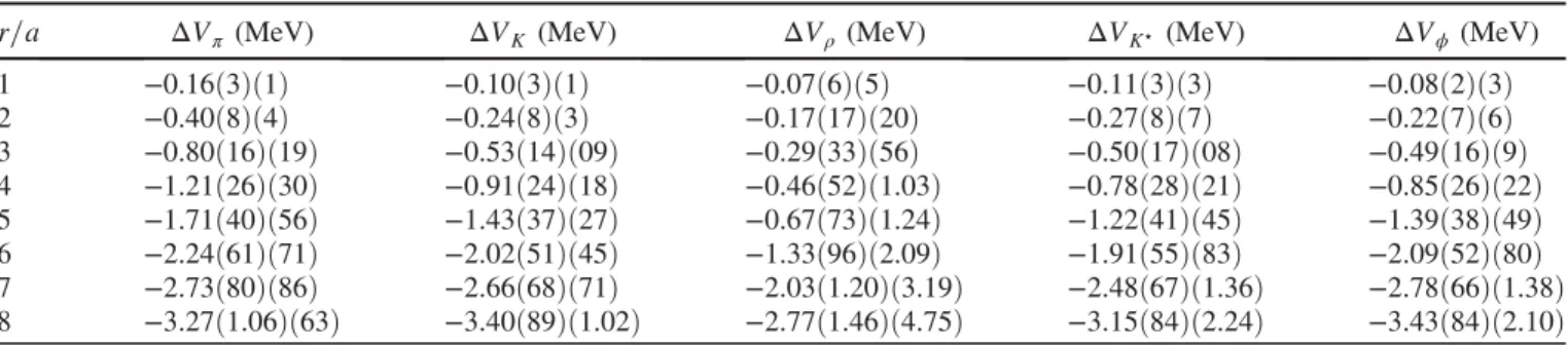
employing a particular polarization to avoid mixing with J¼1=2states. In our case we project ontoJ_z¼3=2with respect to thez axis. We remark that embedding charmonium states within baryons of vanishing strangeness could TABLE I. Values of the difference in the static potential for the mesons, measured atδt¼5a. Errors are statistical and systematic, respectively.

r=a ΔV_π (MeV) ΔV_K (MeV) ΔV_ρ (MeV) ΔV_K⋆ (MeV) ΔV_ϕ (MeV)

1 −0.16ð3Þð1Þ −0.10ð3Þð1Þ −0.07ð6Þð5Þ −0.11ð3Þð3Þ −0.08ð2Þð3Þ 2 −0.40ð8Þð4Þ −0.24ð8Þð3Þ −0.17ð17Þð20Þ −0.27ð8Þð7Þ −0.22ð7Þð6Þ 3 −0.80ð16Þð19Þ −0.53ð14Þð09Þ −0.29ð33Þð56Þ −0.50ð17Þð08Þ −0.49ð16Þð9Þ 4 −1.21ð26Þð30Þ −0.91ð24Þð18Þ −0.46ð52Þð1.03Þ −0.78ð28Þð21Þ −0.85ð26Þð22Þ 5 −1.71ð40Þð56Þ −1.43ð37Þð27Þ −0.67ð73Þð1.24Þ −1.22ð41Þð45Þ −1.39ð38Þð49Þ 6 −2.24ð61Þð71Þ −2.02ð51Þð45Þ −1.33ð96Þð2.09Þ −1.91ð55Þð83Þ −2.09ð52Þð80Þ 7 −2.73ð80Þð86Þ −2.66ð68Þð71Þ −2.03ð1.20Þð3.19Þ −2.48ð67Þð1.36Þ −2.78ð66Þð1.38Þ 8 −3.27ð1.06Þð63Þ −3.40ð89Þð1.02Þ −2.77ð1.46Þð4.75Þ −3.15ð84Þð2.24Þ −3.43ð84Þð2.10Þ

TABLE II. Fit parameters for the difference of the potential for the mesons, see Eq.(14).

MesonH ΔμH(MeV) Δc_Hð10⁻⁴Þ ΔσH (MeV/fm)

π 0.858(39) 2.30(13) −5.75ð11Þ

K 1.167(15) 3.34(52) −5.82ð42Þ

ρ 2.28(38) 6.62(1.31) −10.19ð1.02Þ

K^⋆ 1.38(16) 4.10(59) −6.47ð46Þ

ϕ 1.45(12) 4.18(42) −6.67ð32Þ

0 0.1 0.2 0.3 0.4 0.5 0.6 0.7

−7

−6

−5

−4

−3

−2

−1 0

FIG. 10. The same as in Fig.6for the positive-parity nucleon.

0 0.1 0.2 0.3 0.4 0.5 0.6 0.7

−7

−6

−5

−4

−3

−2

−1 0

FIG. 11. The same as in Fig.6for the positive-parity cascade.

(9)

be an interpretation of the“pentaquark”structures that were recently reported by the LHCb Collaboration [1,2]; for examples see the last paragraph of Sec.III.

In Figs.10,11,12, and13we showΔV_Hðr;δtÞfor the nucleon, the cascade Ξ, the Δ, and the decuplet cascade Ξ, respectively. Again, in all the cases we observe ΔVHðr;δtÞ<0. The results for the positive-parity baryons are collected in TableIIIand are very similar to the values discussed above for the pseudoscalar and vector mesons.

Note, however, that the errors of ΔV in the presence of decuplet baryons become rather large. In particular, this is

so for theΔ, which is why in this case we only show the data up toδt¼5a. The Cornell fit parameters [Eq.(14)] are displayed in TableIV.

3. Negative-parity baryons

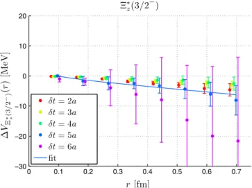
The modification of the potential in the presence of negative-parity baryons appears statistically consistent to the positive-parity case; however, due to the much larger statistical errors, we cannot exclude a more rapid decrease of ΔV_HðrÞ as a function of r. As examples we show in Figs. 14, 15, and 16 the results for the negative-parity

0 0.1 0.2 0.3 0.4 0.5 0.6 0.7

−10

−8

−6

−4

−2 0

FIG. 12. The same as in Fig.6for the positive-parityΔbaryon.

The subscriptzof the baryon label refers to the projection along the Z axisJ_z¼3=2, ensuring no mixing withJ^P¼1=2^þstates takes place.

0 0.1 0.2 0.3 0.4 0.5 0.6 0.7

−10

−8

−6

−4

−2 0

FIG. 13. The same as in Fig. 12 for the positive-parity Ξ^⋆ baryon.

TABLE III. Values of the difference in the static potential for the positive-parity baryons, measured at δt¼5a.

r=a ΔVNð1=2^þÞ(MeV) ΔV_Σð1=2^þÞ (MeV) ΔV_Λð1=2^þÞ(MeV) ΔV_Ξð1=2^þÞ(MeV)

1 −0.24ð8Þð13Þ −0.12ð3Þð10Þ −0.24ð4Þð5Þ −0.12ð3Þð5Þ

6 −2.73ð1.05Þð1.08Þ −2.87ð68Þð91Þ −3.21ð80Þð59Þ −2.67ð61Þð51Þ 7 −3.93ð1.35Þð1.53Þ −3.62ð90Þð1.08Þ −4.19ð1.00Þð1.30Þ −3.54ð78Þð1.00Þ 8 −5.48ð1.67Þð2.28Þ −4.40ð1.16Þð1.47Þ −5.34ð1.23Þð1.84Þ −4.63ð1.01Þð1.80Þ

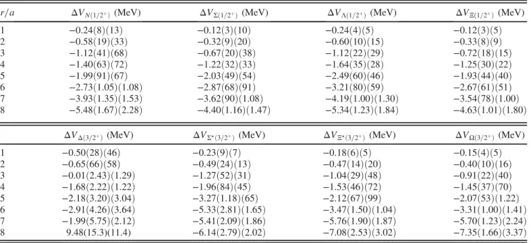
ΔV_Δð3=2^þ_Þ(MeV) ΔV_Σ^⋆_ð3=2^þ_Þ(MeV) ΔV_Ξ^⋆_ð3=2^þ_Þ (MeV) ΔV_Ωð3=2^þ_Þ (MeV)

3 −0.01ð2.43Þð1.29Þ −1.27ð52Þð31Þ −1.04ð29Þð48Þ −0.91ð22Þð40Þ 4 −1.68ð2.22Þð1.22Þ −1.96ð84Þð45Þ −1.53ð46Þð72Þ −1.45ð37Þð70Þ 5 −2.18ð3.20Þð3.04Þ −3.27ð1.18Þð65Þ −2.12ð67Þð99Þ −2.07ð53Þð1.22Þ 6 −2.91ð4.26Þð3.64Þ −5.33ð2.81Þð1.65Þ −3.47ð1.50Þð1.04Þ −3.31ð1.00Þð1.41Þ 7 −1.99ð5.75Þð2.12Þ −5.41ð2.09Þð1.86Þ −5.76ð1.90Þð1.87Þ −5.70ð1.23Þð2.24Þ 8 9.48(15.3)(11.4) −6.14ð2.79Þð2.02Þ −7.08ð2.53Þð3.02Þ −7.35ð1.66Þð3.37Þ

(10)

partners of the nucleon, the cascade, and the decuplet cascade, respectively. The corresponding numerical values for δt¼5a are displayed in Table Vand the Cornell fit parameters in Table VI.

4. Summary

Regardless of meson or baryon, spin, strangeness, or parity, the modifications of the static potential are well described by the parametrization Eq. (14), with the main effects being a reduction of the linear slope and increases of the Coulomb coefficientcand of the offsetμ. All data are consistent with a decrease of the static potential at the distancer¼0.5 fm by about 2–3 MeV.

For r >0.7fm the statistical errors grow substantially as a result of the deteriorating signal-to-noise ratio.

Fortunately, larger distances exceed the size both of charmonium and of the hosting hadron and will not be relevant for the discussion of Sec.VIbelow. However, one may wonder if the reduction persists. In Fig. 17 we show the data for the pion, the kaon, the nucleon, and the cascade up tor≈1.2fm, a distance around which string breaking will occur [39,61]. The decrease of the slope appears to be robust and all large distance data points are consistent with our parametrizations. However, for the more compact pseudoscalar mesons and in particular the kaon the data suggests that above r≈0.8 fm some saturation may set in.

VI. MODIFICATION OF CHARMONIUM BINDING ENERGIES

We have investigated how the static quark-antiquark potential changes in the presence of a light hadron. This is a well-defined observable and the results by themselves are already interesting. However, we wish to go one step further and address possible phenomenological conse- quences. We start with a few words of caution. When it comes to charmonia (and even for bottomonia), relativistic corrections are not small. Moreover, baryons are not particularly light in comparison to the charm quark.

Therefore, for charmonia it may be doubtful if their effect TABLE IV. Fit parameters for the difference of the potential for

the positive-parity baryons, see Eq.(14).

BaryonH ΔμH (MeV) Δc_Hð10⁻⁴Þ ΔσH (MeV/fm) Nð1=2^þÞ 1.17(37) 3.21(1.30) −7.83ð97Þ Σð1=2^þÞ 1.62(21) 4.63(73) −7.99ð60Þ Λð1=2^þÞ 1.28(20) 3.46(69) −8.49ð57Þ Ξð1=2^þÞ 1.54(19) 4.32(75) −7.81ð55Þ Δð3=2^þÞ −0.99ð1.75Þ −2.22ð6.16Þ −0.10ð4.77Þ Σ^⋆ð3=2^þÞ 2.15(37) 6.14(1.30) −11.38ð1.01Þ Ξ^⋆ð3=2^þÞ 1.74(36) 4.90(1.41) −9.40ð1.03Þ Ωð3=2^þÞ 2.34(49) 6.77(1.68) −11.02ð1.41Þ

0 0.1 0.2 0.3 0.4 0.5 0.6 0.7

−30

−20

−10 0 10 20

FIG. 14. The same as in Fig.6for the negative-parity nucleon.

0 0.1 0.2 0.3 0.4 0.5 0.6 0.7

−30

−20

−10 0 10 20

FIG. 15. The same as in Fig.6for the negative-parity cascade.

0 0.1 0.2 0.3 0.4 0.5 0.6 0.7

−30

−20

−10 0 10 20

FIG. 16. The same as in Fig. 12 for the negative-parity Ξ^⋆ baryon.

(11)

can be completely integrated out in a Born-Oppenheimer or adiabatic spirit and put into the quark-antiquark interaction potential. This is less of a problem for the pion and the kaon since M_K=m_c and M_π=m_c are of similar sizes as the squared velocityv²∼0.3. In what follows, we will neglect these effects.

We start from the Schrödinger equation

−∇²

m_cþE_HðrÞ

ψ^ðHÞ_nLðr;θ;ϕÞ ¼M^ðHÞ_nLψ^ðHÞ_nLðr;θ;ϕÞ; ð15Þ where the reduced mass ism_c=2 and

E_HðrÞ ¼2ðm_c−δmÞ þV_HðrÞ ð16Þ

¼2m_cþv₀þΔμH−c_H

r þσHr: ð17Þ In the second step, we have assumed the Cornell parametrization given by Eqs. (10) and (14), where we

set c_H ¼cþΔcH and σH ¼σþΔσH. The parameters ΔμH, Δc_H, and ΔσH specify the modifications of the constant, the Coulomb, and the linear terms, respectively, obtained from the Cornell fits toΔV_HðrÞ ¼V_HðrÞ−V₀ðrÞ carried out in the previous section.

The Cornell parametrization is not valid at large distances due to string breaking effects [39,61] or at small distances where one would expect the coefficientc_Hto run with the scaler. However, we are only interested in mass differencesΔM^ðHÞ_nL ¼M^ðHÞ_nL −M^ð0Þ_nL between a charmonium state with radial and angular momentum quantum numbers nandLrespectively, in the presence of a hadronH, relative

TABLE VI. Fit parameters for the difference of the potential for the negative-parity baryons, see Eq.(14).

BaryonH ΔμH (MeV) Δc_Hð10⁻⁴Þ ΔσH (MeV/fm) Nð1=2⁻Þ −10.18ð6.43Þ −3.50ð22.58Þ 5.39(17.46) Σð1=2⁻Þ 1.88(83) 4.84(2.91) −16.89ð2.26Þ Λð1=2⁻Þ −0.77ð3.51Þ −5.03ð12.61Þ −16.92ð8.93Þ Ξð1=2⁻Þ 4.74(1.18) 14.21(4.11) −20.93ð3.25Þ Δð3=2⁻Þ −23.1ð27.6Þ −69.34ð96.85Þ 94.8(76.2) Σ^⋆ð3=2⁻Þ −0.853ð3.26Þ −12.11ð11.90Þ −30.3ð7.22Þ Ξ^⋆ð3=2⁻Þ −0.23ð1.25Þ −4.37ð4.59Þ −8.92ð2.61Þ Ωð3=2⁻Þ −0.47ð62Þ −1.92ð2.18Þ −0.99ð1.67Þ

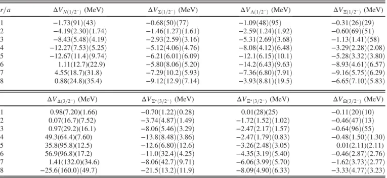
TABLE V. Values of the difference in the static potential for the negative-parity baryons, measured atδt¼5a.

r=a ΔV_Nð1=2⁻_Þ (MeV) ΔV_Σð1=2⁻_Þ (MeV) ΔV_Λð1=2⁻_Þ (MeV) ΔV_Ξð1=2⁻_Þ (MeV)

2 −4.19ð2.30Þð1.74Þ −1.46ð1.27Þð1.61Þ −2.59ð1.24Þð1.92Þ −0.60ð69Þð51Þ 3 −8.43ð5.48Þð4.19Þ −2.93ð2.59Þð3.16Þ −5.31ð2.69Þð3.68Þ −1.13ð1.41Þð58Þ 4 −12.27ð7.53Þð5.25Þ −5.12ð4.06Þð4.76Þ −8.08ð4.12Þð6.48Þ −3.29ð2.28Þð2.08Þ 5 −12.67ð11.4Þð9.74Þ −6.21ð6.01Þð6.09Þ −12.1ð6.15Þð10.1Þ −5.28ð3.32Þð3.80Þ 6 1.11(12.7)(22.9) −5.80ð8.06Þð5.20Þ −14.2ð6.43Þð9.63Þ −8.93ð4.61Þð6.57Þ 7 4.55(18.7)(31.8) −7.29ð10.2Þð5.93Þ −7.36ð6.80Þð7.91Þ −9.16ð5.75Þð6.29Þ 8 0.88(24.8)(35.4) −9.12ð12.9Þð7.14Þ −3.93ð8.81Þð19.5Þ −6.65ð7.10Þð5.83Þ ΔV_Δð3=2⁻_Þ(MeV) ΔV_Σ^⋆_ð3=2⁻_Þ(MeV) ΔV_Ξ^⋆_ð3=2⁻_Þ (MeV) ΔV_Ωð3=2⁻_Þ(MeV)

1 0.98(7.20)(1.66) −0.70ð1.22Þð0.28Þ 0.01(28)(25) −0.11ð20Þð10Þ

2 0.07(16.7)(7.52) −3.74ð4.87Þð1.49Þ −1.72ð1.52Þð1.02Þ −0.46ð47Þð13Þ 3 0.97(29.2)(16.1) −8.06ð5.46Þð3.29Þ −2.47ð2.17Þð1.57Þ −0.64ð96Þð55Þ 4 49.3(64.4)(7.60) −13.8ð8.48Þð3.86Þ −2.47ð1.79Þð0.83Þ −0.48ð1.50Þð1.30Þ 5 35.8(95.8)(12.5) −12.6ð6.80Þð12.6Þ −3.26ð2.48Þð3.05Þ 0.01(2.11)(2.11) 6 56.9(96.8)(17.2) −11.0ð32.4Þð4.25Þ −4.35ð3.19Þð5.40Þ −0.46ð2.87Þð2.76Þ 7 1.41(132.0)(34.6) −8.06ð42.7Þð9.71Þ −6.06ð3.99Þð5.70Þ −1.62ð3.73Þð2.77Þ 8 −25.6ð160.0Þð49.7Þ −21.5ð13.2Þð11.9Þ −8.09ð4.90Þð6.33Þ −3.33ð4.77Þð3.23Þ

FIG. 17. The difference in the static potential for the pion, the kaon, and the positive-parity nucleon and cascade, measured at δt¼5a, up to a distance of 1.2 fm. The curves correspond to the parametrization Eq.(14)with the parameters (obtained by fitting ther <0.7fm data points) displayed in TablesII andIV.

(12)

to the same state in the vacuum. We expect such corrections to affect both masses in similar ways, and therefore to cancel from these differences. The coefficients ΔμH, c_H, andσH are taken from the fits performed in the previous section, while the mass parameterm_c and the offset v₀¼ μ−2δm have to be fixed by matching the energy levels M_nL¼M^ð0Þ_nL, obtained from solving the above Schrödinger equation, to experiment.

Due to the approximations made, our discussion can only be qualitative and hence we neglect our statistical and systematic uncertainties. The central values for the parameters from the Cornell fit to the static potential in the vacuum read [see also Eq. (11)]

σ¼0.0335a⁻²≈ð423MeVÞ²; c¼0.468: ð18Þ Numerically solving the Schrödinger equation and adjust- ingm_c andv₀so that we reproduce the spin-averaged1S and2Scharmonium levels, we find

m_c¼1269MeV; v₀¼113MeV: ð19Þ From Table VII, we see that the above parameters indeed reproduce the experimental1Sand2Slevels; however, we underestimate the 1P mass by 42 MeV. This is due to a combination of overestimating the value of the wave function at the origin, as we neglected running coupling effects, and relativistic corrections[63]; within our approximations, it is not possible to simultaneously reproduce all spin-independent mass splittings within an accuracy better than about 10%.

A negative value of ΔM^ðHÞ_nL means that embedding a charmonium state within the hadron H is energetically favorable, which we interpret as attraction. Unlike in the hydrogen case, the potential is only bound from above by the DD¯ threshold and so it may not be entirely obvious

whether a negative ΔV_HðrÞ results in a positive or a negative shift of the charmonium mass. On one hand, a lowerV_H results in a lowerE_H and therefore in a smaller M^ðHÞ_nL mass. On the other hand, the slope is reduced, resulting in a more extended and less strongly bound wave function.

Before numerically solving the Schrödinger equation we investigate a toy model with a purely linear potential VðrÞ ¼σr. The virial theorem then gives a kinetic energy 2hTi ¼ hrdV=dri ¼σhri ¼2M−2σhri; ð20Þ where we used M¼ hTi þ hVi ¼ hTi þσhri. This means thathri ¼2M=ð3σÞ. The Feynman-Hellmann theorem then gives

∂M

∂σ ¼

∂H

∂σ

¼ hri ¼2M

3σ ; ð21Þ i.e.

ΔM^ð^H^Þ ¼ ðσH−σÞ∂M

∂σ

σ¼σ0

¼2σH

3σ₀M^ð0Þ; ð22Þ whereM^ðHÞ¼MðσHÞ. Therefore, we expect the part of the mass which is due to the interaction,M−2ðm_c−δmÞ, to be lowered by a factor2σH=ð3σÞ, which for our data typically amounts to about 0.4%. As we have neglected Coulomb interactions, we should also neglect the self-energy δm.

Then, using them_cvalue of Eq.(19)andM_1S¼3069MeV, this difference gives 530 MeV. So, for the1Sstate, we expect an attraction ΔM^ðHÞ_1S ≈ −2MeV. Using the experimental 1P–1S and 2S–1S differences lowers this to ΔM^ðHÞ_1P ≈

−3.9MeV andΔM^ðHÞ_2S ≈ −4.5MeV, respectively.

We now solve the Schrödinger equation numerically for the mesons and for some of the positive-parity baryons, using the parameter values of Eqs.(18)and(19), together withΔμH,Δc_H, andΔσHobtained from the fits toΔV_HðrÞ, see TablesIIandIV. The results are collected in TableVII.

Indeed, the masses in all the channels shown are lowered by amounts that are in qualitative agreement with the consid- erations from the virial and Feynman-Hellmann theorems above, and the effect becomes larger for spatially more extended charmonia. Note that the potentials for the ρ meson and the Δ baryon have relatively large errors.

Therefore, the resulting mass shifts statistically agree with those shown for theK and theΞ, respectively.

In Ref.[35], a charmonium-nucleon bound state energy of−20MeV was reported—a factor of 8 larger than our result. The light quark mass employed in that study was approximately 13 times larger than the one we use here.

However, as one can see from TableVII, if we replace the nucleon by the cascade that contains two strange quarks, which are 8 times heavier than our light quark, the binding TABLE VII. Masses and mass differences of spin-averaged

states in MeV taken from experiment[43]and from solving the Schrödinger equation using the Cornell parametrization of our lattice results.

Mass/Mass difference 1S(MeV) 1P(MeV) 2S(MeV) M_nL (experiment) 3068.6 3525.3 3674.4 M_nL (Schrödinger) 3068.6 3483.3 3674.4 ΔM^ðπÞ −1.7 −3.1 −4.0 ΔM^ðKÞ −1.5 −2.9 −3.8 ΔM^ðρÞ −2.5 −4.9 −6.5 ΔM^ð^K^Þ −1.6 −3.2 −4.2 ΔM^ðϕÞ −1.6 −3.2 −4.3 ΔM^ðNÞ −2.4 −4.3 −5.5 ΔM^ðΞÞ −2.0 −3.9 −5.1 ΔM^ðΔÞ −0.9 −1.0 −1.0 ΔM^ðΞ^Þ −2.6 −4.8 −6.3

(13)

appears to become even weaker, albeit by a statistically insignificant difference.

We found that, within the approximations made, the binding of the charmonium1Sstate becomes stronger by values ranging from −1MeV to −2.5 MeV. For the 2S state this effect increases to−1MeV to−6.5MeV. Such estimates will be more reliable for bottomonia where relativistic and m_H=m_b corrections are smaller. However, these states are also less extended spatially and V₀ðrÞ is most strongly modified towards large distances. This means that the mass shifts induced by the presence of a light hadron will be even smaller in the bottomonium case since charmonium and bottomonium binding energies ∼m_Qv² are of similar sizes.

VII. SUMMARY AND OUTLOOK

Studying charmonium resonances above strong decay thresholds poses a considerable challenge to lattice QCD.

In most cases not only radial excitations of the charm quark-antiquark system need to be resolved but also several decay channels open up, at least near the physical values of the light quark mass. Some of the relevant thresholds involve the scattering of three and more hadrons. In this case even the required methodology is under active devel- opment—for recent progress in this direction, see Refs. [64–69]. In view of this, testing specific models or making assumptions in certain limiting cases represents a viable alternative and may provide at least some first- principles insight into the nature of exotic bound states containing hidden charm.

Here we have investigated in the heavy quark limit the hadro-quarkonium picture [22], which assumes quarkonium can be bound inside the core of a light hadron. We employed a single CLS [44] ensemble with N_f¼2þ1 flavors of nonperturbatively order-a-improved Wilson quarks at a lattice spacing a≈0.085fm. The pion and kaon masses are approximately 223 MeV and 476 MeV, respectively; i.e., the light quark mass is by a factor of about 2.7 larger than in nature. Our approach for testing this picture was first to determine the potential between a pair of static sources, approximating a heavy quark-antiquark pair, in the absence of the hadron. Assuming the nonrelativistic limit, the Schrödinger equation can then be solved with this potential in order to obtain (spin-averaged) quarkonium energy levels. This approach can be extended systemati- cally, adding v² corrections, to include heavy quark spin and momentum dependent effects [70–75]. Making the additional assumption that the heavy quark mass is much larger than the mass of the light hadron, the effect of the light hadron onto the quarkonium can also be integrated out adiabatically and cast into the quark-antiquark interaction potential.

We calculated such potentials in the background of a hadronHfor a variety of pseudoscalar and vector mesons, octet and decuplet baryons, and their negative-parity

partners. Of particular interest are the differences ΔV_HðrÞ, relative to the potential in the vacuum. Solving the Schrödinger equation with the modified potential and comparing the outcome to the results obtained in vacuo provides an indication of the strength of the binding between the host hadron and the quarkonium, at least in the heavy quark limit. In principle this approach can also be extended, including mass-dependent corrections and interactions between the spins of the hadron and the heavy quarks. As the effects we detected were quite small, we have, however, no immediate plans of pursuing this line of research.

Resolving very small energy differences was possible by employing a large number of sources on 1552 gauge configurations, corresponding to over 6000 molecular dynamics units of the hybrid Monte Carlo algorithm.

For all the light mesons, namely theπ,K, ρ,K^⋆, and ϕ, as well as the baryons we considered, namely theN,Σ,Λ, Ξ,Δ,Σ,Ξ, andΩof both parities, we foundΔV_HðrÞ<0, suggesting a tendency to bind. The main effect could be quantified as a reduction of the linear slope of the potential.

At a distance of 0.5 fm the potential was lowered by only 2–3 MeV for all these hadrons. Increasing the strangeness resulted in smaller statistical errors but differences between the investigated hadrons were not significant. Translating the modification of the potential into energy levels by solving the Schrödinger equation suggested values for the finite volume binding energy of 1S charmonium ranging from −1 to −2.5MeV and 2S charmonium from −1 to

−6.5MeV, see Table VII. These effects should be even smaller for bottomonia that are most sensitive to modifications of the potential at very short distances.

These binding energies are similar in size to that of deuterium and may be hard to reconcile with the hadroquarkonium picture where the quarkonium is thought to be localized inside the light hadron which has a size ≲1fm. Therefore, in the heavy quark limit, which should at least apply to bottomonia, this may not be a viable picture. We cannot exclude, however, different mechanisms to stabilize hadrocharmonia such as relativistic corrections or corrections due to the mass of the hosting hadron.

The spatial lattice extentL≈4.6=M_π≈4.1fm was not only large relative to the inverse pion mass but also in comparison to the size of a light hadron or a quarkonium state; however, the observed effects were very small.

Hence, a finite-volume study (see, e.g., Ref. [33]) is required to establish if the reported binding energies survive the infinite-volume limit. Simulations on different volumes, and also injecting momentum to enable a scattering study, are ongoing; see Ref.[76]for preliminary results.

Until these more extensive investigations are concluded, we cannot exclude the possibility that no bound state or resonance exists. Therefore, the binding energies presented here should only be considered as upper limits.