Electroproduction of tensor mesons in QCD

JHEP06(2016)039

Published for SISSA by Springer

Received: April 4, 2016 Accepted:May 29, 2016 Published: June 7, 2016

Electroproduction of tensor mesons in QCD

V.M. Braun,^a N. Kivel,^b,1 M. Strohmaier^a and A.A. Vladimirov^a

aInstitut f¨ur Theoretische Physik, Universit¨at Regensburg, D-93040 Regensburg, Germany

bHelmholtz Institut Mainz, Johannes Gutenberg-Universit¨at, D-55099 Mainz, Germany

E-mail: vladimir.braun@ur.de,kivel@kph.uni-mainz.de, matthias.strohmaier@ur.de,aleksey.vladimirov@ur.de

Abstract: Due to multiple possible polarizations hard exclusive production of tensor mesons by virtual photons or in heavy meson decays offers interesting possibilities to study the helicity structure of the underlying short-distance process. Motivated by the first measurement of the transition form factor γ^∗γ → f2(1270) at large momentum transfers by the BELLE collaboration we present an improved QCD analysis of this reaction in the framework of collinear factorization including contributions of twist-three quark-antiquark- gluon operators and an estimate of soft end-point corrections using light-cone sum rules.

The results appear to be in good agreement with the data, in particular the predicted scaling behavior is reproduced in all cases.

Keywords: QCD Phenomenology, NLO Computations ArXiv ePrint: 1603.09154

1On leave of absence from St. Petersburg Nuclear Physics Institute, 188350, Gatchina, Russia.

JHEP06(2016)039

Contents

1 Introduction 1

2 f2(1270) production in two-photon reactions 3

3 Distribution amplitudes 4

4 QCD factorization 9

5 Soft (end-point) contributions 11

6 Results and discussion 14

A Other conventions 17

B Scale dependence 19

C Equations of motion 20

D QCD sum rules 21

E f_g^S from the radiative decay Υ(1S) →γf₂ 25

1 Introduction

In recent years there has been increasing interest to hard exclusive production of tensor mesons a₂(1320), K₂^∗(1430), f₂(1270) and f₂⁰(1520) by virtual photons or in heavy meson decays. In particular the possibility of three different polarizations of tensor mesons in weakB meson decays can shed light on the helicity structure of the underlying electroweak interactions. A different symmetry of the wave function and hence a different hierarchy of the leading contributions for the tensor mesons as compared to the vector mesons can lead to the situations that the color-allowed amplitude is suppressed and becomes compa- rable to the color-suppressed one. This feature can give an additional handle on penguin contributions. The early work was devoted mainly on the identification of the interesting decay modes and their basic theoretical description using various factorization techniques at the leading-order and the leading-twist level, see e.g. [1–6]. These studies are to a large extent exploratory. The physics potential of tensor meson production will depend on the accuracy of the theoretical description of such processes that can be achieved in QCD.

The recent study [7] of hard exclusive production of tensor mesons in single-tag two- photon processes is an important step forward in this context. This is a “gold-plated”

reaction where the theoretical formalism can be tested and the relevant nonperturbative

JHEP06(2016)039

functions — tensor meson distribution amplitudes (DAs) — determined, or at least con- strained. Our work aims to match this experimental progress with a development of the robust QCD framework for the study of the transition form factor γ^∗γ → f₂(1270) in collinear factorization.

This reaction has already attracted some attention. Useful kinematic relations and estimates of the transition form factors for the mesons built of light and heavy quarks can be found in [8]. In ref. [9] it was pointed out that hard exclusive production of f2(1270) with helicity λ = ±2 is dominated by the gluon component in the meson wave function and can be used to determine gluon admixture in tensor mesons in a theoretically clean manner. In ref. [10] the helicity difference sum rule for the weighted integral of the γ^∗γ fusion cross section was derived and shown to provide constraints on the transition form factor in question. A phenomenological model for the tensor meson form factor can also be found in [11]. A related reaction γ^∗γ → ππ near the threshold has been discussed in [12–14].

Theory of the transition form factors goes back to the classical work on hard exclusive reactions in QCD [15–17]. The case of tensor mesons does not bring in complications of principle as compared to the pseudoscalar meson transition form factors that have been studied in great detail, but the tensor meson case is much less developed on a technical level. Our paper can be viewed as a major update of a earlier work [9] where the leading contributions to this process have been identified and calculated at the leading order. The new elements are:

• We introduce twist-three and twist-four DAs and calculate the corresponding contri- butions to the form factors;

• We calculate meson mass corrections terms in the higher-twist DAs and estimate the leading “genuine” three-particle contributions;

• We include the next-to-leading (NLO) corrections and calculate the charm-loop con- tribution for the helicity amplitude with λ=±2 taking into account for thec-quark mass;

• We estimate quark-gluon coupling constants entering on the higher-twist level using QCD sum rules and the leading-twist gluon couplings using QCD sum rules and, alternatively, from the quarkonium decay Υ(1S)→γ f2;

• We estimate the soft (end-point) correction for the leading, helicity-conserving am- plitude.

The main conclusion from our study is that the experimental results on theγ^∗γ→f2(1270) transition form factors reported in ref. [7] appear to be in a very good agreement with the QCD scaling predictions starting already at moderateQ² '5 GeV². This is in contrast to the transition form factors for pseudoscalar π, η, η⁰ mesons where large scaling violations have been observed [18–20]. The absolute normalization for all helicity form factors can be reproduced assuming a 10–15% lower value of the tensor meson coupling to the quark

JHEP06(2016)039

energy-momentum tensor as compared to the estimates existing in the literature, which is well within the uncertainty.

The presentation is organized as follows. Section 2 is introductory. It contains the definition of helicity amplitudes for theγ^∗γ →f2(1270) transition and the necessary kine- matic relations. For the reader’s convenience, the relation of our conventions to other def- initions existing in the literature is explained in appendix A. Section 3 contains a detailed discussion of the leading-twist and higher-twist DAs of the tensor meson, which are the main nonperturbative input in the calculations. This section contains several new results.

The relevant nonperturbative parameters are calculated in appendix D using QCD sum rules. In appendix E we estimate one of the leading-twist gluon couplings from the decay Υ(1S)→γ f₂. In section 4 we calculate the three existing helicity amplitudes in collinear factorization, including higher-twist and, partially, radiative corrections. In section 5 we discuss the power suppressed corrections ∼ 1/Q² arising from the end-point regions. We explain how such corrections can be estimated using dispersion relations and duality and construct the light-cone sum rule for the largest, helicity conserving amplitude. In section 6 we compare our results to the experimental data [7] and summarize.

2 f₂(1270) production in two-photon reactions

We consider the reaction

γ^∗(q₁) +γ(q₂)→f₂(P), q₁²=−Q², q₂²= 0, P²=m² (2.1) with one real and one virtual photon, P =q₁+q₂. Here and below m= 1270 MeV is the meson mass.

The transition amplitude can be related to the matrix element of the time-ordered product of two electromagnetic currents

Tµν =i Z

d⁴x e^−iq1xhf₂(P, λ)|T{j_µ^em(x)j_ν^em(0)}|0i, (2.2) where

j_µ^em(x) =e_uu(x)γ¯ _µu(x) +e_dd(x)γ¯ _µd(x) +. . . .

The correlation functionTµνcan be decomposed in contributions of three Lorentz structures T^µν =T₀^µν+T₁^µν+T₂^µν, (2.3) defined as

T₀^µν =e^(λ)∗_αβ −g^µν_⊥

(q1−q2)^α(q1−q2)^β m²

(2q1q2)²T0(Q²), T₁^µν =e^(λ)∗_αβ (−g^αν_⊥ ) (q1−q2)^β

q₁^µ−q₂^µ q²₁ (q1q2)

m²

(2q1q2)²T1(Q²), T₂^µν =e^(λ)∗_αβ

g^αµ_⊥ g^βν_⊥ − 1

2g_⊥^µν m²

(2q₁q₂)²(q1−q2)^α(q1−q2)^β

T2(Q²). (2.4)

JHEP06(2016)039

Here

g_⊥^µν =g^µν− 1

(q₁q₂)(q^µ₁q^ν₂ +q^ν₁q₂^µ) + q₁²

(q₁q₂)²q₂^µq₂^ν, 2q₁q₂ =m²+Q². (2.5) The polarization tensore^(λ)_αβ is symmetric and traceless, and satisfies the conditione^(λ)_αβP^β = 0. Polarization sums can be calculated using

X

λ

e^(λ)_µνe^(λ)∗_ρσ = 1

2MµρMνσ+1

2MµσMνρ−1

3MµνMρσ, (2.6) where M_µν = g_µν −P_µP_ν/m² and the normalization is such that e^(λ)_µνe^(λ_µν^0)∗ = δ_λλ⁰. The invariant form factors T0,T1 and T2 correspond to the three possible helicity amplitudes

T₀ : γ^∗(±1) +γ(±1)→f₂(0), T₁ : γ^∗(0) +γ(±1)→f₂(∓1),

T₂ : γ^∗(±1) +γ(∓1)→f₂(±2). (2.7) All three amplitudes (form factors) have mass dimension equal to one and scale asT_k ∼Q⁰ (up to logarithms) in theQ²→ ∞ limit. The two-photon decay width off₂(1270) is given by [21]

Γ[f2→γγ] = πα² 5m

2

3|T₀(0)|²+|T₂(0)|²

= 3.03(40) keV, (2.8) whereα'1/137 is the electromagnetic coupling constant. Assuming that|T₂(0)| |T₀(0)|

we obtain

|T₂(0)| ' r5m

πα² Γ[f₂→γγ] = 339(22) MeV. (2.9) The relation of our definition of helicity form factors to the other existing in the literature definitions is given in appendixA.

3 Distribution amplitudes

In the standard classification the tensorJ^{P C} = 2⁺⁺SU(3)_f nonet is composed off₂(1270), f₂⁰(1525), a₂(1320) and K₂^∗(1430). Isoscalar tensor states f₂(1270) and f₂⁰(1525) have a dominant decay mode in two pions (or two kaons). The isovector a2(1320) decays only in three pions and is more difficult to observe in hard reactions. In the quark model these mesons are constructed from a constituent quark-antiquark pair in the P-wave and with the total spin equal to one. In QCD they can be represented by a set of Fock states in terms of quarks and gluons, that further reduce to DAs in the limit of small transverse separations.

In the exact SU(3)-flavor symmetry limit the f2(1270) meson is part of a flavor-octet, f2 =T8, andf₂⁰(1525) is a flavor-singlet,f₂⁰ =T1. However, it is known empirically that the SU(3)-breaking corrections are large. Since f₂(1270) andf₂⁰(1525) decay predominantly in ππ andKK, it follows that they are close to the nonstrange and strange flavor eigenstates, respectively, with a small mixing angle, see [21,22]. In this paper we assume ideal mixing at a low scale which we take to beµ₀= 1 GeV, for definiteness. In other words, we assume

JHEP06(2016)039

thatf₂(1270) at this scale is a pure nonstrange isospin singlet. This assumption can easily be relaxed when more precise data on the form factors become available. In what follows the notation ¯q . . . qrefers to the SU(2)-flavor-singlet combination

¯ q q= 1

√2

u u¯ + ¯d d

, (3.1)

whereu ansdare the usual “up” and “down” quark flavors.

Let n^µbe an arbitrary light-like vector, n² = 0, and p_µ=P_µ−1

2n_µm²

pn , g^⊥_µν =g_µν− 1

pn n_µp_ν+n_νp_µ

. (3.2)

We define the f2-meson quark-antiquark light-cone DAs as matrix elements of nonlocal light-ray operators [9,23]

hf₂(P, λ)|¯q(z₂n)γ_µq(z₁n)|0i = f_qm² e^(λ)∗nn

(pn)²p_µ Z 1

0

du e^izu12(pn)φ₂(u, µ) +f_qm²e^(λ)∗_⊥µn

pn Z ₁

0

du e^iz12u(pn)g_v(u, µ)

−1

2n_µf_qm⁴ e^(λ)∗_nn (pn)³

Z 1 0

du e^iz12u(pn)g₄(u, µ), hf₂(P, λ)|¯q(z₂n)γ_µγ₅q(z₁n)|0i = −if_qm²_µναβn^νp^α

pn e^(λ)∗_βn

pn Z 1

0

du e^iz12u(pn)g_a(u, µ),(3.3) where

e^(λ)∗_µn ≡e^(λ)∗_µν n^ν, e^(λ)∗_⊥µn≡g_µν^⊥e^(λ)∗_νn =e^(λ)∗_µn −p_µe^(λ)∗nn

(pn) + 1

2n_µe^(λ)∗_nn m²

(pn)² (3.4) and we use a shorthand notation

z₁₂^u = ¯uz1+uz2, u¯= 1−u . (3.5) Note that

e^(λ)∗_pn =−1

2e^(λ)∗_nn m²

pn . (3.6)

In all expressions light-like Wilson lines between the quark fields are implied.

The DAs defined in (3.3) satisfy the following symmetry relations:

φ₂(u) =−φ₂(¯u), g_v(u) =−g_v(¯u), g_a(u) = +g_a(¯u), g₄(u) =−g₄(¯u). (3.7) and are normalized as

Z 1 0

du(2u−1)φ₂(u) = Z 1

0

du(2u−1)g_v(u) = Z 1

0

du(2u−1)g₄(u) = 1. (3.8)

JHEP06(2016)039

The integral of the DA g_a(u) vanishes Z 1

0

du g_a(u) = 0, (3.9)

and the first nonzero (second) moment, R1

0 du(2u −1)²g_a(u), involves contributions of three-particle operators, see below.

The coupling fq is defined as the matrix element of the local operator 1

2hf₂(P, λ)|¯qh

γ_µi^↔Dν +γ_νiD^↔µ

iq|0i=f_qm²e^(λ)∗_µν (3.10) whereD^↔µ=D^→µ−D^←µis the covariant derivative. This coupling is scale dependent and gets mixed with the gluon coupling and the similar coupling for strange quarks. In appendixB we summarize the scale dependence of all DA parameters introduced in this section.

The numerical value off_q has been estimated in the past [23–25] (see also appendixD) using the QCD sum rule approach. Another possibility is to use the experimental result on the decay width Γ(f2 → ππ) and estimate fq assuming that the matrix element of the energy-momentum tensor hπ⁺π⁻|Θ_µν|0i is saturated by the tensor meson [23–27]. These two estimates agree with each other surprisingly well, although this agreement should not be overrated as in both cases the non-resonant two-pion background is not taken into account. We use (cf. [23] and appendix D)

f_q = 101(10) MeV (3.11)

(at the scale 1 GeV) as the default value for the present study. Note that the positive sign for this coupling is a phase convention, whereas the relative signs of the other matrix elements with respect to f_q are physical and can be determined by considering suitable correlation functions as explained in appendix D.

Using the definitions in (3.3) it is easy to derive the operator product expansion (OPE) of quark bilinears close to the light cone x² →0 (at the tree level):

hf₂(P, λ)|¯q(x)γµq(−x)|0i

=fqm² e^(λ)∗xx

(P x)²Pµ

Z 1 0

du ei(2u−1)(P x)

φ2(u)−gv(u) +1

4x²m²φ4(u)

+fqm²e^(λ)∗µx

P x Z 1

0

du ei(2u−1)(P x)gv(u) +1

2f_qm⁴x_µ e^(λ)∗_xx (P x)³

Z 1 0

du ei(2u−1)(P x)h

2g_v(u)−φ₂(u)−g₄(u)i , hf₂(P, λ)|¯q(x)γ_µγ₅q(−x)|0i

=−if_qm²_µναβx^νP^α P x

e^(λ)∗_βx P x

Z 1 0

du ei(2u−1)(P x)g_a(u), (3.12) where φ4(u) is another twist-four two-particle DA that can be expressed in terms of the other functions using QCD equations of motion (EOM), see below.

JHEP06(2016)039

In addition we define three-particle twist-three DAs as g^µµ_⊥ ⁰hf₂(P, λ)|¯q(z3n)igG_µ⁰_n(z2n)/nq(z1n)|0i=fqm²(pn)e^(λ)∗_⊥µn

Z

Dα e^ipnPαkzkΦ3(α), g^µµ_⊥ ⁰hf₂(P, λ)|¯q(z₃n)gGe_µ⁰_n(z₂n)nγ/ ₅q(z₁n)|0i=f_qm²(pn)e^(λ)∗_⊥µn

Z

Dα e^ipnPαkzkΦe₃(α). (3.13) The conformal expansion of the three-particle DAs reads [28,29]

Φ₃(α) = 360α₁α²₂α₃

ζ₃+ 1

2ω₃(7α₂−3) +. . .

, Φe₃(α) = 360α₁α²₂α₃

0 +1

2eω₃(α₁−α₃) +. . .

. (3.14)

The two-particle DAs g_a(u) and g_v(u) have collinear twist three and contain con- tributions of geometric twist-two and twist-three operators.¹ The contributions of lower geometric twist are traditionally referred to as Wandzura-Wilczek (WW) contributions.

They can be calculated in the terms of the leading-twist DA φ₂(u) as [9,23]

g_v^{W W}(u) = Z u

0

dv φ₂(v)

¯ v +

Z 1 u

dv φ₂(v) v , g_a^{W W}(u) =

Z u 0

dv φ₂(v)

¯ v −

Z 1 u

dv φ₂(v)

v . (3.15)

Assuming for simplicity the asymptotic expression for the leading-twist quark DA

φ^as₂ (u) = 30u(1−u)(2u−1), (3.16) one obtains

g_v^{W W}(u) = 3C₁^1/2(2u−1) + 2C₃^1/2(2u−1),

g_a^{W W}(u) = 5C₂^1/2(2u−1), (3.17)

where Cn^1/2(x) are Legendre polynomials. The Legendre expansion can be motivated by the properties of these DAs under conformal transformations [28, 29]. The “genuine”

geometric twist-three contributions can be related to the three-particle DAs using EOM, see appendixC. For the truncation in (3.14) one obtains

g_a(u) =g^{W W}_a (u)−10ζ₃C₂^1/2(2u−1) +15

8 (ω₃−ωe₃)C₄^1/2(2u−1), g_v(u) =g^{W W}_v (u)−

10ζ₃−15

8 (ω₃−eω₃)

C₃^1/2(2u−1). (3.18)

1We remind that geometric twist is defined as “dimension minus spin” of the corresponding operators, whereas collinear twist is defined as “dimension minus spin projection on the light-ray direction”. The collinear twist counting is closely related to the counting of powers of large “plus” components of meson momentum in the matrix elements and determines power suppression of the corresponding contributions at largeQ², see e.g. ref. [29].

JHEP06(2016)039

The twist-three matrix elements can be estimated using QCD sum rules, see appendix D.

We obtain (at the scale 1 GeV)

ζ₃ = 0.15(8), ω₃=−0.2(3), ωe₃= 0.06(1). (3.19) The DAs φ4(u) and g4(u) have collinear twist four and receive contributions of the geometric twist-two, -three and -four operators. The Wandzura-Wilczek-type twist-two contributions assuming the asymptotic expression for φ2(u) (3.16) have the form

φ^{W W}₄ (u) = 100u²(1−u)²(2u−1),

g^{W W}₄ (u) = 30u(1−u)(2u−1). (3.20) We expect that these contributions are the dominant source of the power-suppressed correc- tions∼1/Q²because of the large mass of thef2(1270) and will neglect “genuine” geometric twist-three and twist-four contributions. The derivation of the expressions in (3.20) pro- ceeds similar to the case of the DAs of vector mesons considered in [28,30,31] so that we omit the details.

Finally, the leading-twist gluon DAs of f2(1270) can be defined as [9]

g^µµ_⊥ ⁰g_⊥^νν0hf₂(P, λ)|G^a_nµ0(z₂n)G^a_nν0(z₁n⁰)|0i

=f_g^T

e^(λ)_⊥µν(pn)²−1

2g^⊥_µνm²e^(λ)_nn Z 1

0

du e^iz12upnφ^T_g(u)

−f_g^Sm²g_µν^⊥e^(λ)_nn Z 1

0

du e^izu12pnφ^S_g(u). (3.21) The distribution amplitudes φ^T_g(u) and φ^S_g(u) are both symmetric to the interchange of u↔u¯and describe the momentum fraction distribution of the two gluons in the f₂-meson with the same and the opposite helicity, respectively. The asymptotic distributions at large scales are equal to

φ^T,as_g (u) =φ^S,as_g (u) = 30u²(1−u)². (3.22) The normalization constantsf_g^T andf_g^Sare defined through the matrix element of the local two-gluon operator:

hf₂(P, λ)|G^a_αβ(0)G^a_µν(0)|0i = f_g^T

(P_αP_µ−1

2m²g_αµ)e^(λ)_βν −(α↔β)

−(µ↔ν)

−1 2f_g^Sm²

g_αµe^(λ)_βν −(α↔β)

−(µ↔ν)

. (3.23) The couplingf_g^S can be estimated from the radiative decay Υ(1S)→γf2, see appendixE.

The result is consistent with the assumption that f_g^S is very small at hadronic scales and is generated mainly by the evolution. In the numerical analysis we use the value

f_g^S(1 GeV) = 0. (3.24)

JHEP06(2016)039

(q

1 )

(q

2 )

f

2 (P)

(q

1 )

(q

2 )

f

2 (P) (q

1 )

(q

2 )

f

2 (P)

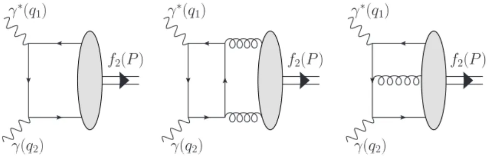
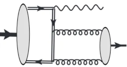
Figure 1. Leading contributions to the transition form factors γ^∗γ→f2(1270) in QCD. Adding crossing-symmetric diagrams is implied.

The coupling to a helicity-aligned gluon pair, f_g^T, is difficult to quantify. The calculation of the leading contributions to the relevant correlation functions suggests that the two couplings,f_g^S and f_g^T, have the same sign, see appendix D. In what follows we use

f_g^T(1 GeV)≈20 MeV (3.25)

as a ballpark estimate.

As already mentioned, all couplings considered here are scale dependent. The relevant expressions are collected in appendix B.

4 QCD factorization

QCD description of the transition form factors in two-photon reactions is based on the analysis of singularities in the product of two electromagnetic currents in (2.2) in the limit (x−y)² → 0. Typical Feynman diagrams contributing to the leading-order accuracy are shown in figure1.

The leading contributions in theQ²→ ∞limit have been calculated already in [9]. The form factor T₀(Q²) is of the leading twist and is dominated by the quark DA. In this case we include, in addition, NLO perturbative corrections to the leading twist contribution, which can be extracted from the corresponding expressions for the two-pion production in [13]. We also include the twist-four meson-mass correction m²/Q² which is a new result.

The form factor T₁(Q²) is of twist-three. It receives the Wandzura-Wilczek-type con- tributions calculated in [9] and the “genuine” twist-three contributions of three-particle quark-antiquark gluon DAs (new result).

As already noticed in [9], the T₂(Q²) form factor is rather peculiar: the leading con- tribution at Q² → ∞ comes in this case from the two-gluon DA with aligned helicity that we refer to as gluon transversity DA. However, this contribution is suppressed by the factor αs/π∼0.1 which is the standard perturbation theory factor for an extra loop, and also the two-gluon coupling to a “conventional” quark-antiquark meson is expected to be small as compared to the quark-antiquark coupling. By this reason the true QCD asymptotics for this form factor may be postponed to very large momentum transfers that are out of reach on the existing experimental facilities. The result for T2(Q²) given below includes the leading term and the Wandzura-Wilczek-type higher-twist power correction

JHEP06(2016)039

that does not involve such small factors. We also calculate and add the leading-twist c-quark contribution.

With these new additions, the expressions for the form factors are T₀ = hf_qi

Z 1 0

du

¯ u

1 +α_s

4πCq(u)

φ₂(u)− α_s 4π 2 3f_g^S

Z 1 0

duC^S_g(u)φ^S_g(u) +2m²

Q² hf_qi Z 1

0

du

¯ u

ulnu φ₂(u)− 1 8¯uφ₄(u)

, (4.1)

T1 = 2hf_qi Z 1

0

du

¯ u

h

gv(u)−ga(u)i

= 4hf_qi Z ₁

0

du

¯

u ln(u)φ₂(u) + 2hf_qi Z

DαCΦ(α)

Φ₃(α) +Φe₃(α)

, (4.2)

T₂ = 4m² Q² hf_qi

Z 1 0

dulnu g_v(u) +α_s π f_g^T

Z 1 0

du

¯ u

2 3 +4

9Cc(u)

φ^T_g(u), (4.3) where the notation hf_qi stands for the sum of the light quark couplings weighted with the electromagnetic charges

hf_qi= 4

9f_u(µ) +1

9f_d(µ) +1

9f_s(µ) = 5√ 2

18 f_q(µ) +1

9f_s(µ). (4.4) The coefficient function of the three-particle DAs to T1 is given by

CΦ(α) = 1 α2

1 α1α¯1

+ 1 α2

lnα₁

¯ α1

− ln ¯α₃ α3

+lnα₁

¯ α²₁

, (4.5)

and the NLO quark and gluon coefficient functions forT0 read [13]

Cq(u) =CF

ln²u¯+ 3 lnu−9

, C^S_g(u) = 2 lnu uu¯²

ulnu−2u−2

. (4.6)

The c-quark contribution to T2(Q²) (this is a new result) is given by Cc(u) = 1 +2m²_c

Q²

−β u¯uln

β+ 1 β−1

+β_u

¯ u ln

β_u+ 1 βu−1

+β_u¯

u ln

β_u¯+ 1 βu¯−1

(4.7) + 1

uu¯ 1

2 +m²_c Q² ln²

β+ 1 β−1

−ln²

βu+ 1 β_u−1

−ln²

βu¯+ 1 β_u¯−1

, where

βu= s

1 +4m²_c

uQ² , β≡β1. (4.8)

Here mc '1.4 GeV is thec-quark mass. We did not calculate the corresponding contribu- tion toT0(Q²) because in this case it is a part of aO(α_s) correction to the leading-order result O(1). It turns out (see below) that the c-quark contribution to T₂ is still strongly suppressed as compared to the light quarks in the Q² range of the Belle experiment, so that taking it into account forT0 does not seem to be worth the effort at this stage in view of the other uncertainties.

JHEP06(2016)039

We have checked the electromagnetic gauge invariance of our results by explicit calcu- lation. Note that electromagnetic Ward identities relate the contributions of three-particle DAs, the last diagram in figure1, to the higher-twist contributions in the first diagram en- coded in the “genuine” twist-three contributions to the two-particle DAs. Such terms can be thought of as corresponding to gluon emission from the quark legs in the hard scattering amplitude. Thus it is not surprising that the twist-three form factorT₁(Q²) can be written in two equivalent representations as in (4.2): either contributions of the three-particle DAs can be eliminated in favor the two particle ones, or, vice verse, the “genuine” twist-three contributions to the two-particle DAs can be rewritten in terms of the three-particle DAs.

Evaluating (4.1), (4.2), (4.3) using the expressions for the DAs that are collected in the previous section we obtain

T₀ = 5

1− α_s 27π

hf_qi − 215 27

α_s

π f_g^S−5m²

Q²hf_qi, (4.9)

T1 = 10 3 hf_qi

1 + 4ζ3+ 9

16(ω3−ω˜3)

, (4.10)

T2 = 10 3

m² Q²hf_qi

2−ζ3+ 3

16(ω3−ω˜3)

+ 5 2

αs

π f_g^T 2

3+ 4

9λ(m²_c/Q²)

, (4.11) where all nonperturbative parameters and the QCD coupling have to be taken at the hard scale µ∝ Q. The function λ(m²_c/Q²) takes into account suppression of the charm quark contribution in comparison to the light flavors; it is given by

λ(x) = 1−30x−72x²+ 24x(1 + 3x)βbln βb+ 1 βb−1

!

−6x 1 + 6x+ 12x²

ln² βb+ 1 βb−1

! , (4.12) whereβb=√

1 + 4x. The normalization is such thatλ(0) = 1. Note thatλ(0.1)'0.091 so that thec-quark contribution atQ² ∼20 GeV²is still suppressed by an order of magnitude as compared to the contributions ofu,d,squarks.

The expressions for the helicity form factors collected in this section present our main result.

5 Soft (end-point) contributions

Transition form factors with one real photon receive power corrections ∼ 1/Q² coming from the region of large separation (x−y)² ∼ 1/Λ²_QCD between the electromagnetic cur- rents in (2.2). Such contributions are missing in the OPE and involve overlap integrals of the nonperturbative light-front wave functions at large transverse separations between the constituents and cannot be calculated in terms of DAs. They are revealed, nevertheless, as end-point divergences in the momentum fraction integrals in the framework of QCD factorization if one tries to extend it beyond the leading power accuracy. Such divergences are a clear indication that some extra contributions have to be added.

The technique that we adopt in what follows has been suggested originally [32] for the γ^∗γ → π⁰, see [33, 34] for two recent state-of-the-art analysis. In this section we

JHEP06(2016)039

demonstrate how the same approach can be applied to the production of tensor mesons (cf. [35]). To this end we consider the simplest example: the form factor T0 to the leading- order accuracy, leaving the NLO corrections to T₀ and the other two form factors,T₁ and T₂, for a future study. Our presentation follows closely the work [33] where further details and generalizations can be found.

The idea is to calculate the transition form factor for two large virtualities q₁²=−Q², q₂² =−q², Q² q²,

using collinear factorization or, equivalently, OPE, and perform analytic continuation to the real photon limit q² = 0 using dispersion relations. In this way explicit evaluation of contributions of the end-point regions is avoided (since they do not contribute for suffi- ciently large q²) and effectively replaced by certain assumptions on the physical spectral density in the q²-channel.

For our purposes it is sufficient to assume that the second photon is transversely polarized. Then there are no new Lorentz structures and the only difference is that the form factors depend on two virtualities. The starting point is that the form factor

Tb0(Q², q²) = 1

(2q1q2)² T0(Q², q²), T0(Q²)≡(m²+Q²)²Tb0(Q², q² = 0), (5.1) satisfies an unsubtracted dispersion relation in the variable q² for fixedQ². Separating the contribution of the lowest-lying vector mesonsρ, ω one can write

Tb₀^{γ∗γ∗→f2}(Q², q²) =

√2f_ρTb₀^γ∗ρ→f2(Q²) m²_ρ+q² + 1

π Z ∞

s0

dsImTb₀^{γ∗γ∗→f2}(Q²,−s)

s+q² , (5.2) wheres₀ is a certain effective threshold. Here we assumed that the ρ andω contributions are combined in one resonance term and the zero-width approximation is adopted; f_ρ ∼ 200 MeV is the usual vector meson decay constant. Since there are no massless states, the real photon limit is recovered by the simple substitution q² →0 in this equation.

If both virtualities are large, Q², q² Λ²_QCD, the same form factor can be calculated using OPE. Assume this calculation is done to some accuracy. The result is an analytic function that satisfies a similar dispersion relation

Tb_0,OPE^{γ∗γ∗→f2}(Q², q²) = 1 π

Z ∞ 0

dsImTb_0,OPE^{γ∗γ∗→f2}(Q²,−s)

s+q² . (5.3)

The basic assumption of the method is that the physical spectral density above the thresh- olds0 coincides (if integrated with a smooth test function) with the spectral density calcu- lated in OPE, in the very similar way as the total cross section of e⁺e⁻-annihilation above the resonance region coincides with the QCD prediction,

Tb_0,OPE^{γ∗γ∗→f2}(Q²,−s)'Tb₀^{γ∗γ∗→f2}(Q²,−s), s > s₀. (5.4) We expect that OPE becomes exact as q² → ∞ so that in this limit the calculation has to reproduce the “true” form factor. Equating the two representations in eqs. (5.2), (5.3) at

JHEP06(2016)039

q² → ∞and subtracting the contributions of s > s₀ from the both sides one obtains

√

2f_ρTb₀^γ∗ρ→f2(Q²) = 1 π

Z _s0

0

dsImTb_0,OPE^{γ∗γ∗→f2}(Q²,−s). (5.5) This relation explains whys0 is usually referred to as the interval of duality (in the vector channel). The (perturbative) QCD spectral density ImTb_0,OPE^{γ∗γ∗→f2}(Q²,−s) is a smooth func- tion, very different from the physical spectral density ImTb₀^{γ∗γ∗→f2}(Q²,−s) ∼ δ(s−m²_ρ).

Nevertheless, their integrals over a certain region of energies coincide. In this sense QCD description of correlation functions in the terms of quark and gluons is dual to the descrip- tion in the terms of hadronic states.

In practical applications one uses a certain trick [36] which allows to reduce the sen- sitivity on the duality assumption in (5.4) and simultaneously suppress contributions of higher twists in the OPE. This is done going over to the Borel representation 1/(s+q²)→ exp[−s/M²] the net effect being the appearance of an additional weight factor under the integral that suppresses the large invariant mass region:

√

2f_ρTb₀^γ∗ρ→f2(Q²) = 1 π

Z _s0

0

ds e^{−(s−m2ρ)/M2}ImTb_0,OPE^{γ∗γ∗→f2}(Q²,−s). (5.6) Varying the Borel parameter M² within a certain window, usually 1–2 GeV² one can test sensitivity of the results to the particular model of the spectral density.

With this refinement, substituting eq. (5.6) in (5.2) and using eq. (5.4) one obtains for q² →0 (cf. [32])

Tb_0,LCSR^γ∗γ→f2(Q²) = 1 π

Z s0

0

ds

m²_ρe^{(m2ρ−s)/M2}ImTb_0,OPE^{γ∗γ∗→f2}(Q²,−s) + 1

π Z ∞

s0

ds

s ImTb_0,OPE^{γ∗γ∗→f2}(Q²,−s). (5.7) The abbreviation LCSR stands for the Light-Cone Sum Rules [37], as this approach is usually referred to.

Adding and subtracting the contribution ofs < s₀in the second term,² one can rewrite the result as

Tb_0,LCSR^γ∗γ→f2(Q²) = Tb_0,OPE^γ∗γ→f2(Q²) +Tb_0,soft^γ∗γ→f2(Q²), (5.8) where the first term is the original OPE expression which is possible but not necessary to write in the dispersion representation, and the second term is the correction of interest:

Tb_0,soft^γ∗γ→f2(Q²) = 1 π

Z s0

0

ds s

s

m²_ρe^{(m2ρ−s)/M2} −1

ImTb_0,QCD^{γ∗γ∗→f2}(Q²,−s). (5.9) An attractive feature of this technique is that one does not need to evaluate the non- perturbative wave function overlap contributions explicitly: they are taken into account effectively via the modification of the spectral density.

2Such a rewriting is not always possible as the separation of the OPE result and the soft correction can suffer from end-point divergences, see [33].

JHEP06(2016)039

As an illustration, consider the leading-twist QCD result at the leading order in strong coupling:

Tb₀(Q², q²) = hf_qi Z 1

0

du φe₂(u)

[¯uQ²+uum¯ ²+uq²]², (5.10) where

φe₂(u) =− Z u

0

dv φ₂(v), φe^as₂ (u) = 15u²u¯². (5.11) This expression can easily be brought to the form of a dispersion relation changing variables u→s= ^u_u^¯Q²+ ¯um²and integrating by parts. In this way one obtains after some rewriting,

Tb_0,soft^γ∗γ→f2(Q²) = −hf_qi Z 1

u0

duφb2(u)

"

1

[¯uQ²+uum¯ ²]² −e^{(m2ρ−s)/M2} m²_ρu²M²

#

+hf_qi 1

m²_ρe^{(m2ρ−s0)/M2} − 1 s0

φb2(u0)

u²₀m²+Q², (5.12) where

u₀= 1 2m²

hp(Q²+s₀−m²)²+ 4m²Q²−(Q²+s₀−m²)i

, (5.13)

and, for comparison, to the same accuracy Tb_0,OPE^γ∗γ→f2(Q²) =hf_qi

Z 1 0

du φb2(u)

[¯uQ²+u¯um²]². (5.14) Note thatu0→1 asQ² → ∞so that the integration region shrinks to the end-pointu→1 and the correction is power suppressed∼1/Q²in this limit, as expected. Numerical results are presented in the next section.

6 Results and discussion

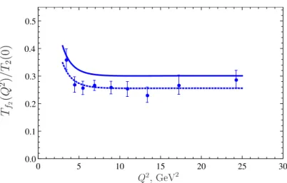
The effective form factor averaged over polarizations T_f2(Q²) =

s 2 3

T₀(Q²) T2(0)

2

+ Q²m² (m²+Q²)²

T₁(Q²) T2(0)

2

+

T₂(Q²) T2(0)

2

, (6.1)

is calculated using default values of the nonperturbative parameters and compared with the experimental data [7] in figure 2. We observe a perfect scaling behavior for Q² & 4–

5 GeV² as predicted by QCD, whereas the normalization is slightly off — about 1–1.5σ if systematic errors in the data are taken into account. This difference can easily be compensated by a 10–15% decrease of the value of the quark coupling fq which serves as an overall normalization factor in the calculation, or, alternatively, by a moderate deviation of the leading twist DA φ2(u) from its asymptotic form. For illustration we show in the same figure by short dashes the result of the QCD calculation with fq = 85 MeV at the scale 1 GeV.

JHEP06(2016)039

è

è è è è è è

è è

0 5 10 15 20 25 30

0.0 0.1 0.2 0.3 0.4 0.5

Q 2

;GeV 2 Tf2

(Q

2 )=T2

(0)

Figure 2. The effective form factor summed over polarizations normalized to T₂(0) = 339 MeV.

The calculation using default values of the nonperturbative parameters is shown by the solid curve.

The same calculation with the quark coupling fq reduced by 15% is shown by short dashes. The experimental data are taken from ref. [7]. Only statistical errors are shown.

Such a 10–15% smaller coupling as compared to our default value fq = 101 MeV is certainly possible as the existing estimates are not reliable. A more precise number can eventually be obtained from lattice QCD, however, this calculation is rather complicated and will take time. It would be very interesting to measure the time-like transition form factor e⁺e⁻ → f2(1270)γ at large virtualities q² ∼100 GeV² (cf. [38]) where the nonper- turbative uncertainties are considerably reduced. This would give a direct measurement of thefq-coupling.

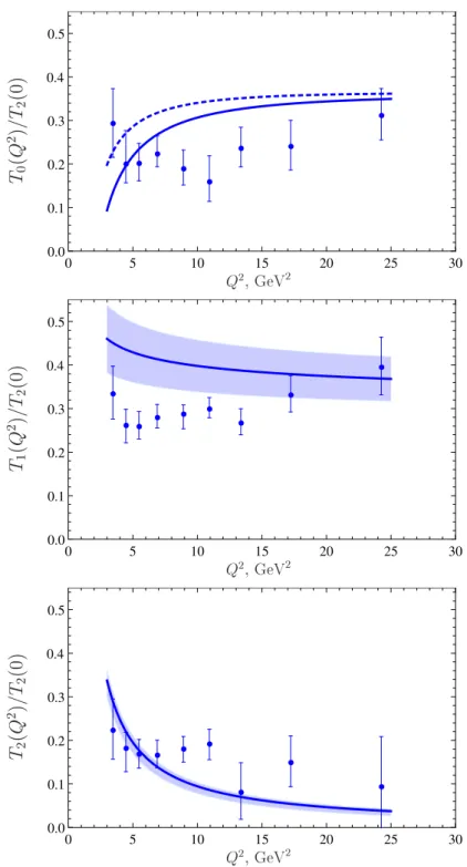
Our results for the helicity-separated form factors T₀(Q²), T₁(Q²), T₂(Q²) are com- pared with the experimental data [7] in figure3. All three form factors are described rather well, the QCD calculation being slightly above the data as we have already seen for the helicity-averaged form factor in figure 2. Note that our result forT₁(Q²) only includes the leading-power contribution at large Q² in contrast to T₀(Q²) and T₂(Q²) where we also calculated the 1/Q² correction. Terms∼1/Q² inT1(Q²) correspond to collinear-twist-five and soft contributions and are more difficult to estimate. They should be expected, how- ever, to be negative and of the same order of magnitude as forT2(Q²) so that the increase of the QCD curve forT1(Q²) in figure3at smallerQ² will almost certainly be compensated by power corrections and is not a reason for concern. As expected, T₁(Q²) is also more sensitive to the twist-three quark-antiquark-gluon contributions as compared to the other two form factors, and the uncertainties in the corresponding parameters are not negligible, they are shown by the shaded area.

As discussed in [9], the form factorT2(Q²) at asymptotically largeQ² is dominated by the two-gluon contribution with aligned helicity that we refer to as gluon transversity DA.

This contribution is suppressed, however, by the factor α_s/π ∼0.1 which is the standard penalty for an extra loop. Also the two-gluon coupling to a “conventional” quark-antiquark meson is unlikely to be large as compared to the quark-antiquark coupling. By this reason, T₂(Q²) at realisticQ²is still dominated by the Wandzura-Wilczek-type higher-twist power correction that does not involve such small factors: the shaded area in the plot forT2(Q²)

JHEP06(2016)039

è è è è

è è

è è

è

0 5 10 15 20 25 30

0.0 0.1 0.2 0.3 0.4 0.5

Q 2

;GeV 2 T0

(Q

2 )=T2

(0)

è

è è è è è è

è

è

0 5 10 15 20 25 30

0.0 0.1 0.2 0.3 0.4 0.5

Q 2

;GeV 2 T1

(Q

2 )=T2

(0)

è

è è è è è è

è

è

0 5 10 15 20 25 30

0.0 0.1 0.2 0.3 0.4 0.5

T2

(Q

2 )=T2

(0)

Q 2

;GeV 2

Figure 3. The form factorsT₀(Q²),T₁(Q²), T₂(Q²) (from top to bottom) normalized to T₂(0) = 339 MeV. The result for T₀(Q²) shown by the solid line includes the estimate of soft end-point contributions using light-cone sum rules. The result without the soft correction is shown by dashes.

The error band for T1(Q²) (shaded area) corresponds to variation of the twist-three parameters in the range specified in (3.19), whereas for T₂(Q²) we also include variation of the tensor gluon couplingf_g^T in the range±50 MeV. The experimental data are taken from ref. [7]. Only statistical errors are shown.