What can be learned from the transition form factor of γ ∗ γ ∗ → η : feasibility study

(1)

https://doi.org/10.1140/epjc/s10052-019-6824-2

Regular Article - Theoretical Physics

What can be learned from the transition form factor of γ ^∗ γ ^∗ → η : feasibility study

Yao Ji^a, Alexey Vladimirov^b

Institut für Theoretische Physik, Universität Regensburg, 93040 Regensburg, Germany

Received: 30 January 2019 / Accepted: 30 March 2019 / Published online: 9 April 2019

Abstract We present an analysis of the recent measurement ofη-meson production by two virtual photons made by the BaBar collaboration. It is the first measurement of a transition form factor which is entirely within the kinematic regime of the collinear factorization approach, and it thus provides a clean test of the QCD factorization theorem for distribution amplitudes (DAs). We demonstrate that the data are in agreement with perturbative QCD. Also we show that it is sensitive to power corrections to the factorization theorem and to the decay constants. We discuss features of the meson production cross-section and point out the kinematic regions that are sensitive to interesting physics. We also provide an estimation of uncertainties on the extraction of DA parameters.

1 Introduction

Recently, the measurement of the two-photon-fusion reaction e⁺(pa)+e⁻(pb)→e⁺(p1)+e⁻(p2)+η(p_η) (1) in the double-tag mode has been reported by the BaBar collaboration [1]. These data open the possibility of studying the meson-transition form factorF(Q²₁,Q²₂)with both photon virtualities being large,Q²₁_,₂ Λ²_QCD. In fact, it is the first measurement of photon-production of a meson where the QCD factorization theorem could be applied in a truly perturbative regime. Being the opening analysis of this kind, the data [1] have large uncertainties and could not provide any significant restrictions on the models for DAs. However, this is only the first step to a promising future. In this work, we analyze the data [1] within the QCD factorization approach and explore opportunities granted by such double-tag measurements.

ae-mail:yao.ji@ur.de

be-mail:alexey.vladimirov@physik.uni-regensburg.de

On the theory side, the description of the form factor with both non-zero virtualitiesF(Q²₁,Q²₂)is essentially simpler in comparison to the description of the form factor with a real photon F(Q²,0). The latter has been measured by several experiments [2–6], and has also been the subject of many theoretical studies; see e.g. [7–10]. The simplification comes from the fact that all interaction vertices are within the perturbative regime of QCD (whereas forF(Q²,0)one must include description for non-perturbative interaction of a quark with the real photon). Therefore, the data [1] provide a clean test of the factorization approach. Our analysis demonstrates agreement between the measurement and the theory expectations, if one includes higher-twist corrections.

There are several important questions about the meson structure that could be addressed with the help ofF(Q²₁,Q²₂).

The two most prominent are: the validity of the state-mixing picture for hard processes, and the size of the gluon com- ponent. In this work we demonstrate that the current level of experimental precision is not sufficient to resolve these questions, however, it allows the determination ofη–ηstate- mixing constants. In the last part of the paper, we point out the kinematic regions of cross-section that are sensitive to var- ious parameters, and discuss the uncertainty reduction for theory parameters with the increase of the data precision.

2 Theory input

The cross-section for the process (1) is given by [11,12]

dσ

dQ²₁dQ²₂ = α_em⁴

2s²Q²₁Q²₂|F(Q²1,Q²₂)|²Φ(s,Q²₁,Q²₂), (2) wheres =(pa+pb)²,(pa,b−p1,2)² = −Q²₁_,₂, and Fis theγ^∗γ^∗→ηtransition form factor. The functionΦaccu- mulates the information about lepton tensor and the phase volume of the interaction. For completeness we present its explicit form in Appendix A.

(2)

In the case of large-momentum transfer, the form factor Fcan be evaluated within perturbative QCD. In our analysis we consider the leading-twist contribution and the leading power-suppressed contribution, which originates from the twist-3, twist-4 distribution amplitudes (DAs) and the meson- mass correction. To this accuracy, the form factor reads F=Ftw−2+Ftw−3+Ftw−4+FM +O(Q⁻⁶), (3) where we omit the arguments(Q²₁,Q²₂, μ)of the form factors for brevity. In the following we provide minimal details on the theory input to our analysis.

Leading-twist contribution. The leading-twist contribution has the following form:

Ftw−2(Q²1,Q²₂, μ)

=

i

C_ηⁱ(μ)

₁

0

dx T_Hⁱ (x,Q²₁,Q²₂, μ)φⁱ_η(x, μ), (4)

whereiis the label that enumerates variousSU(3)and flavor channels,C_ηⁱ are axial-vector couplings (decay constants), T_Hⁱ is the coefficient function, andφ_ηⁱ is the DA for a given channel.

In our analysis we have considered the NLO expression for the leading-twist contribution. At this order, one has singlet (i =1)and octet(i =8)quark channels, and the (singlet) gluon channel(i =g). Coefficient functions for the singlet and octet channels are the same,T_H¹ =T_H⁸, and at LO read T_H¹(x,Q²₁,Q²₂, μ)=T_H⁸(x,Q²₁,Q²₂, μ)

= 1

x Q²₁+ ¯x Q²₂ +(x↔ ¯x)+O(αs);

(5) here and in the following we use the shorthand notation

¯

x =1−x. The NLO expression for quark and gluon (T_H^g) coefficient functions have been evaluated in [13] and [14], respectively.

We use the assumption that at the low-energy reference scale μ0 = 1 GeV, the singlet and octet DAs coincide, φ¹(x, μ0) = φ⁸(x, μ0). However, generally, singlet and octet DAs are different since they obey different evolution equations. In particular, the singlet DAφ¹(x)mixes with the gluon DAφ^g(x). Therefore, the gluon contribution must also be accounted for, even if the gluon DA is taken to be zero at the reference scale. The evolution equations and anoma- lous dimensions at NLO can be found in [15–17] (for the collection of formulas see also Appendix B in Ref. [8]). It is well known that it is convenient to present DAs as series of Gegenbauer polynomials. The twist-2 quark and gluon DAs for (pseudo)scalar mesons are

φ_η^q(x, μ)=6xx¯

∞

n=0,2,...

a^q_n_,η(μ)C³n^/²(2x−1), (6)

φ_η^g(x, μ)=30x²x¯²

∞

n=2,4,...

a_n^g_,η(μ)Cn⁵^/²(2x−1). (7)

In the following we omit the subscriptη, since it is the only case considered in this work. Coefficients of such an expan- sion do not mix under evolution at LO, however, they do mix at NLO. The leading asymptotic coefficienta₀^q=1 and does not evolve, which corresponds to electro-magnetic current conservation. Typically, it is assumed that the coefficients of the higher Gegenbauer modes are smaller than the lower ones. In our analysis we include thea₂^q_,₄anda₂^gmodes (while we do take into account higher modes during the evolution procedure).

FKS scheme. We use the Feldmann–Kroll–Stech (FKS) scheme for the definition of the couplingsC_ηⁱ [18,19]. The FKS scheme assumes that theη–ηsystem can be described as an ideal¹mixing of SU(3)-flavor states (singlet and octet).

Therefore, the couplingsC_η⁽ⁱ⁾ can be expressed in terms of quark couplings with a mixing angle

C¹_η(μ)=C_η^g(μ)=2 9(√

2fqsinϕ0+ fscosϕ0), (8) C_η⁸ = fqsinϕ0−√

2fscosϕ0

9√

2 . (9)

The values of the quark couplings fq, fs, and of the mixing angleϕ0are specified later.

We stress that the couplingC¹_η does depend on the scale μ(whereas the octet couplingC_η⁸ does not). Its dependence appears at NLO due to U(1) anomaly [20] and reads C¹_η^,^g(μ)=C_η¹^,^g(μ0)

1+2nf

πβ0(αs(μ)−αs(μ0)

, (10) where nf is the number of active flavors. The inclusion of this scale dependence is important for intrinsic consistency of the NLO approximation, but also numerically sizable, e.g.

the evolution from 1 GeV to 10 GeV changes the value of the coupling by almost 9%.

Target mass correction and higher-twist contributions. As we will demonstrate later, it is important to include the power- suppressed contributions in this energy region. These contributions, namely twist-3, twist-4, and the leading meson-mass corrections, have been derived in Ref. [8] in the case of double virtual photons (see also [21]). The expressions of these suppressed contributions have the generic form

1 Namely, the coupling constants and wave functions share the same mixing parameters.

(3)

Fig. 1 The distribution of bins in the(Q²₁,Q²₂)plane. Black lines and numbers correspond to bins measured in [1]. Gray dashed lines correspond to extra binning during the generation of pseudo-data

FX(Q²₁,Q²₂, μ)=

_∞

0

ds

q=u+d,s

cq

ρ⁽_X^q_,η⁾(Q²₁,s, μ) s+Q²₂ , (11) wherecu+d = 5√

2/9 andcs =2/9. The explicit expressions for the spectral density functionsρ can be found in Ref. [8] as Eqs. (82), (83) and (84) forρM,ρtw−3andρtw−4, respectively. The important feature of these corrections is that they all depend on the leading-twist Gegenbauer coeffi- cientsanin Eq. (6). Importantly, the meson-mass correction does not contain any additional non-perturbative constants, but only parameters from the twist-2 contribution.

The twist-3 and twist-4 corrections have extra parameters, calledh⁽_η^q⁾andδ_η⁽^q⁾. We have used the following values for these constants, determined in [22,23]:

h⁽_η^u^,^d⁾=0, h⁽_η^s⁾=(0.5 GeV²)× f_η⁽^s⁾, (12) (δ⁽_η^u^,^d⁾)²=(δ_η⁽^s⁾)²=0.2 GeV². (13) Strictly speaking, these constants were derived for the case of pion DAs; however, we use these values due to the absence of analogous analysis forη. In our study, we have also dropped the quark-mass corrections since they only produce a tiny numerical effect.

3 Analysis of the data

The measurement [1] provides the differential cross-section dσ/dQ²₁dQ²₂ofe⁺e⁻→e⁺e⁻ηmeasured in five bins. The energy range of the bins is shown in Fig.1. The total energy coverage is 2 < Q²₁_,₂ < 60 GeV², totally in the range of applicability for the perturbation theory. However, the area of the bins is large and thus, in order to compare the theory cross-section (2) with the data, we average the theoretical

predictions over each bin. The averaging procedure is essen- tial for such a kind of analysis and could not be replaced by considering the cross-section as a weighted average. This is especially true for the diagonal bins, since the contributions of higher Gegenbauer moments have a negligible value at the diagonal Q²₁=Q²₂.

Input parameters. The shape ofηDA is not very well stud- ied; therefore, there are no commonly accepted values of higher Gegenbauer coefficients. For this initial study we have taken the values discussed in [8]. There are three models regarding the leading-twist coefficients,

MODEL 1: a₂^q=0.10, a₄^q= 0.1, a₂^g= −0.26, MODEL 2: a₂^q=0.20, a₄^q= 0.0, a₂^g= −0.31, MODEL 3: a₂^q=0.25, a₄^q= −0.1, a₂^g= −0.22. (14) In all these models, thes quark coefficients is assumed to be the same as their u/d-quark counterparts. The models are determined at the reference scaleμ0 = 1 GeV. As for the higher-twist corrections, we take the values presented in Eqs. (12) and (13). In Ref. [8] it was shown that these models are in agreement with the values of the form factorF(Q²,0) measured by CLEO [5] and BaBar [6].

Other important inputs are the values of the quark couplings fq,sand theη–ηstate-mixing angleϕ0, defined in the FKS scheme. There are several studies of these parameters.

The original work [18] yields

FKS:

fq =(1.07±0.02)f_π, fs =(1.34±0.06)f_π, ϕ0=39.3^o±1.0^o.

(15)

Here and in the following f_πis the pion decay constant f_π = 103.4±0.2 MeV. A later analysis by Escribano and Freri (EF) [24] gives

EF:

fq =(1.09±0.03)f_π, fs =(1.66±0.06)f_π, ϕ0=40.7^o±1.4^o.

(16) Finally, the most recent analysis by Fu-Guang Cao (FGC) [25] found

FGC:

fq=(1.08±0.04)f_π, fs =(1.25±0.08)f_π, ϕ0=37.7^o±0.7^o.

(17)

All these analyses use different data sets and different assumptions and thus are competitive to each other.

Test of the theory. In Table1, we show the values ofχ²per number of points (five in this case) evaluated within different models. Comparison of values of cross-section (for MODEL 1) is given in Fig.2.

One can see from Table1that, despite the fact that the data are rather poor, they already are rather selective. In particular, the data completely disregard the EF values of the iso-spin

(4)

Table 1 Values ofχ²/#points evaluated for different theoretical inputs in MODEL 1. The fifth and sixth columns represent values without power corrections (both mass and higher twist) and without higher- twist corrections, respectively

MODEL 1 MODEL 2 MODEL 3 No pow.

corr.

No tw.

3–4 corr.

FKS 1.11 1.16 1.18 1.64 1.29

EF 1.83 1.92 1.98 3.12 2.29

FGC 0.97 1.00 1.02 1.35 1.08

Fig. 2 Comparison of values of cross-section evaluated in MODEL 1 with different iso-spin coupling parameters to the values of measured cross-section

couplings. It also prefers the FGC values of parameters to the FKS one. It is worth pointing out that this conclusion is preliminary due to the poor quality of the current data, but we expect such measurements with lower uncertainties in the future play a key role in determining the quark couplings and the state-mixing angle. Also we see that the data are sensitive to the power corrections, especially to the meson-mass

correction. We recall that the meson-mass correction does not have any new parameters, apart from the state-mixing coupling and DA of the leading twist. The higher-twist corrections incorporate parametersh^q andδ^q in Eqs. (12) and (13), which in principle, could be extracted from such measurements.

For FKS and FGC values with power corrections included, we observe perfect agreement of the data with the theory.

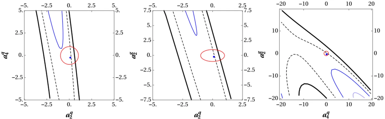
However, current measurement is not sensitive enough with respect to parameters of DA. All models given in Eq. (14) produce similar results. Moreover, the landscape of theχ² function is rather inclusive (see Fig. 3) and therefore does not allow determination of DA moments. In Fig.3, one can see that the parametersaⁱ_nare strongly correlated in the current data set, and this does not even allow for an accurate determination of the error band. It is a rather unfortunate but predictable conclusion. Indeed, from the five presented bins only two are significantly influenced by the parameters of DAs, as we show in the next section.

4 Feasibility study

In this section, we would like to demonstrate the potentials of the double-tag measurements and point out interesting kinematic regions sensitive to one or another physics. In what follows, we use MODEL 1 (with power corrections) with FGC values of state-mixing couplings as the theory input.

Sensitivity to the theory parameters. First of all, it is interesting to analyze the regions ofQ²regarding their sensitivity to different theory input. With this aim, we vary the values of parametersanby a fixed amount±0.4, so thatχ²/#points does not significantly deviates from 1, and plot the relative changes of the cross-section (in percentage); see Fig.4. We

Fig. 3 The landscape of theχ²function evaluated for data [1] with FGC parameters in the planes of the DA moments. The dashed line corresponds to the valueχ²/5=1, the black (blue) line corresponds to χ²=6(4). The blue dot corresponds to the values of MODEL 1. The

red circle designates the approximate region of the theoretical expecta- tion for DA parameters. In each plot, two relevant moments of the DA are varied, while the third one is taken from MODEL 1

(5)

Fig. 4 The cross-section variation with respect to the change of a parameter in the(Q²₁,Q²₂)plane. Gray lines show the binning of the data. The values are adjusted to the intensity of the color as in Fig.5

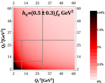
Fig. 5 The cross-section variation with respect to the change of the twist-3/4 parameterh^q_ηin the(Q²₁,Q²₂)plane. Gray lines show the binning of the data. The variation of cross-section by changing parameter δ^q_η±0.1GeV is practically the same

observe that at the diagonal section(Q²₁ = Q²₂)the cross- section is practically independent on higher Gegenbauer moments.²Their influence on the cross-section increases to the border of the phase-spaceQ²_i →0. Naturally, the coefficienta₂^qgives the most important contribution, whereas the contributions ofa₂^ganda^q₄ are smaller. The dependence on the gluon parametera₂^gis less rapid than the dependence on the parametera₄^q. Therefore, it influences already the diagonal bins. The measurements of the off-diagonal sector (while staying away from the boundary) would allow one to decor- relate the constantsa₂^ganda^q₄.

2In fact, one can check that the convolution ofT_Hwith thenth Gegen- bauer moment is proportional to(Q²₁−Q²₂)^[ⁿ^/²^]at NLO [26]. Thus, the corrections to an asymptotic DA necessarily vanish at the diagonal.

The similar plot for the sensitivity of the cross-section to the twist-3/4 parameters is shown in Fig.5(Here, we demonstrate only the variation of the parameterh^q. The variation of parameterδ^qresults in an almost identical plot). As expected, these parameters are important in the region of small Q1,2

(i.e., 2 GeV² Q²₁_,₂ 10 GeV²). What is less expected is that the cross-section’s dependence, though small (of the order of 2%), still remains at largeQ²₁_,₂.

It is clear that the diagonal values play a special role. In fact, the leading-twist contribution of the diagonal bins are entirely determined by the asymptotic quark DA,φ^q(x) = 6xx. Thus,¯ the diagonal bins are the perfect laboratory to determine the couplings Cⁱ_η (decay constants). Also, by studying the dependence of diagonal values onQ²=Q²₁= Q²₂one can accurately extract the higher-twist parameters, such ashandδ.

Estimation of parameter error bars. As we have seen in the previous section, current measurement does not allow for a meaningful extraction of the DA parameters, due to the large error bars and large size of binning at present. Therefore, it is interesting to study the effective size of the error bars with respect to different binning and statistics. To perform this analysis we have generated 100 replicas of pseudo-data and estimated the average errors on the parameter extraction. The results of the estimation are presented in Table2.

To generate the pseudo-data we have used the central values predicted by the theory (FGC, MODEL 1), and distributed them with the errorsα·δσ, whereδσis the statistical uncertainty of measurement reported in [1]. The systematic uncertainty is taken to be 12% (as in [1]). The error estimation is made by averaging over replicas with the boundary ofχs²±1 for a given parameter withχs²equal to the number of data points. Forα=1 the error estimation produces values similar to the one plotted in Fig.3, if one ignores the correlation effects. Considering the dynamics of the error-

(6)

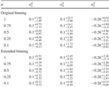
Table 2 Estimate of the determination uncertainty on the leading-twist parametersa_nfrom the pseudo-data (see text). The parameterαis the relative size of the systematic uncertainty with respect to the original one

α a₂^q a₄^q a₂^g

Original binning

1 0.1⁺_−1.89¹^.⁰² 0.1⁺_−5.68²²^.⁵ −0.26⁺_−13.5⁶^.⁹³ 0.75 0.1^+0.73₋₁_.₇₃ 0.1^+14.1₋₅_.₄₇ −0.26^+4.90₋₁₁_.₄ 0.5 0.1⁺_−0.97⁰^.⁶⁵ 0.1⁺_−5.89³^.⁵⁴ −0.26⁺_−6.41⁴^.⁴⁰ 0.25 0.1^+0.56₋₀_.₄₀ 0.1^+1.88₋₂_.₉₇ −0.26^+3.79₋₂_.₆₁ 0.1 0.1⁺_−0.13⁰^.³⁸ 0.1⁺_−0.62¹^.⁷³ −0.26⁺_−0.82²^.⁴⁵ Extended binning

1 0.1⁺_−1.89⁰^.⁵³ 0.1⁺_−9.33²^.⁴⁵ −0.26⁺_−11.3³^.³⁸ 0.75 0.1⁺_−1.24⁰^.³⁹ 0.1⁺_−6.09¹^.⁷⁹ −0.26⁺_−7.84²^.⁴⁸ 0.5 0.1^+0.36₋₀_.₇₂ 0.1^+1.64₋₃_.₁₈ −0.26^+2.25₋₄_.₄₃ 0.25 0.1^+0.22₋₀_.₃₂ 0.1^+0.89₋₁_.₂₂ −0.26^+1.47₋₂_.₈₃ 0.1 0.1⁺_−0.12⁰^.¹² 0.1⁺_−0.49⁰^.⁴⁸ −0.26⁺_−0.86⁰^.⁷⁴

reduction, we conclude that the original binning is not very efficient. Even reducing statistical uncertainties by a factor of 10, we are still not able to extract the DA parameters better than an order of magnitude. The reason is that there are only two bins sensitive to variation of these parameters (bins 3 and 4).

We have also considered the pseudo-data generated for an alternative split of the data in nine bins. The additional energy-bins are shown in Fig.1by dashed lines. To generate the pseudo-data in this case, we have taken the central values predicted by the theory, and the systematic uncertainty is given byα·δσ, withδσtaken from the original bin in the percentage (with an original overall systematic uncertainty).

With this binning the uncertainties in the extraction of param- etersandecrease, as shown in the second part of Table2. The uncertainties for the parametersa₄^qanda₂^gstill remain large.

In essence, a finer binning allows a more accurate determination of thea^q₂ constant. It suggests that with a simi- lar measurement for γ^∗γ^∗ → η, one can put the state- mixing hypothesis for DAs to the test.Indeed, the diagonal bins would provide an accurate determination of the state- mixing constant, whereas off-diagonal bins determine a^q₂ for η andη independently. It is worth mentioning that it is also possible to extract the Gegenbauer moments of the leading-twist DA from γ^∗γ → η/η. In this case, however, certain theoretical assumptions must be made to access the non-perturbative regime of QCD which introduces additional theoretical uncertainties. We, therefore, argue that the double-virtual measurements provide a cleaner probe for the moments and have the potential to be competitive once the data are refined.

5 Conclusion

We have analyzed the recently measured cross-section of e⁺e⁻→e⁺e⁻ηin the double-tag mode. This measurement gives access to theηtransition form factor with both non- zero virtualitiesF(Q²₁,Q²₂). It allows one for the first time to test the factorization approach for the transition form factor in the perturbative regime. We have found that the data are in total agreement with the perturbative QCD prediction as well as with a previous analysis made for the form factor with one photon on-shellF(Q²,0).

Since the provided data have large uncertainties, it is not sufficient for a detailed study of leading-twist DA parameters. However, it is sensitive to power corrections (mostly to the meson-mass corrections), which should be included in the analysis to describe the data. It is also very selective for the coupling constants and mixing angle in the FKS scheme and therefore has great potential in determining this parameters once the uncertainty of the data is reduced. In particular, we have shown that values extracted from [24] deviate significantly from this measurement.

We have also presented the study regarding the sensitivity of particular parameters to different regions in the(Q²₁,Q²₂) plane. We have demonstrated that the diagonal values (Q²₁= Q²₂) of the cross-section are practically independent of the higher moments of the leading-twist DA and are entirely described by its asymptotic form. This makes this kinematic region ideal for the determination of theη/ηdecay constants and related parameters. At small values of Q²₁ = Q²₂, the diagonal region with 2 GeV² Q²₁_,₂ 10 GeV²presents the clean measurement of higher-twist parameters where the QCD perturbative approach is applicable. The sensitivity to the higher-twist parameters is especially interesting due to the planned accurate extraction of these parameters from QCD lattice calculations [27].

The off-diagonal values of the cross-section are important for the determination of parameters of the leading-twist DA.

We have found that the current binning is not sufficient for such an analysis, and in fact, even a decrease of the statistical uncertainty by a factor of 10 could not help in determining these interesting parameters within a reasonable range. The main reason for the large uncertainties is the strong correlation between the parameters for quark and gluon DAs. We point out that in comparison toγ^∗γ →ηprocess, the pro- cessγ^∗γ^∗ → η provides a cleaner probe for the parameters as it is completely in the perturbative regime of QCD and therefore has less theoretical uncertainties. One could, however, significantly increase the precision in parameter determination with finer off-diagonal bins. In particular, it is realistic to expect an accurate determination ofa₂^q(the second Gegenbauer moment of the leading-twist quark DA). In this case, it would be the first measured parameter for the η-meson DA (we recall that nowadays DAs forη and η

(7)

meson are typically taken equal to those of theπ-meson, due to a lack of data). Moreover, if the measurement of the form factor forγ^∗γ^∗→ ηbecomes available, it will allow us to test the state-mixing hypothesis directly on the level of wave functions at short distances.

Acknowledgements We thank V. Braun for multiple discussions, multiple remarks and general enthusiasm. A.V. also thanks V.P. Druzhinin for correspondence.

Data Availability StatementThis manuscript has no associated data or the data will not be deposited. [Authors’ comment: All produced data are presented in plots and tables within article.]

Open Access This article is distributed under the terms of the Creative Commons Attribution 4.0 International License (http://creativecomm ons.org/licenses/by/4.0/), which permits unrestricted use, distribution, and reproduction in any medium, provided you give appropriate credit to the original author(s) and the source, provide a link to the Creative Commons license, and indicate if changes were made.

Funded by SCOAP³.

Appendix A: Kinematic factors

The functionΦoriginates from the convolution of the photons polarization tensor and the lepton tensor together with the volume of the phase-space integration of an unstable par- ticle. For the process

e⁺(pa)+e⁻(pb)→e⁺(p1)+e⁻(p2)+η(p_η), it reads

Φ(s,−t1,−t2)= 1 π

dW²ds1ds2

√B

−Δ4

×m²_η W

Γ_η

(W²−m²_η)²+Γ_η²m²_η, (A.1) wheres1,2=(p1,2+p_η)²,t1,2=(pa,b−p1,2)²= −Q²₁_,₂, W²=p²_η,m_ηandΓ_ηare the mass and decay width of theη state. The factorBhas been derived in [11,12] and depends on the angular modulation distribution of electrons. For the integrated case (i.e. for a spherical distribution) it reads B= 1

16(t1t2[(m²_η+4s−2s1−2s2+t1+t2)² +(t1+t2−m²_η)²−4t1t2] −4[s(t1+t2)

+(s2−t1)(s1−t2)−sm²_η]). (A.2) The functionΔ4is the Gram determinant,

16Δ4

=

0 s −t1 s−s1+t2

s 0 s−s2+t1 −t2

−t1 s−s2+t1 0 s−s1−s2+m²_η s−s1+t2 −t2 s−s1−s2+m²_η 0

. (A.3)

Its null-lines define the boundary of the integration overs1,2.

In the narrow-width approximation the integral over W can be removed and the factor simplifies (see also [28]), Φ(s,−t1,−t2)=

ds1ds2

√B

−Δ4

. (A.4)

This integral can be taken explicitly in terms of elementary functions.

References

1. J.P. Lees et al., Phys. Rev. D98(11), 112002 (2018).https://doi.

org/10.1103/PhysRevD.98.112002

2. C. Berger et al., Phys. Lett.142B, 125 (1984).https://doi.org/10.

1016/0370-2693(84)91147-X

3. H. Aihara et al., Phys. Rev. Lett.64, 172 (1990).https://doi.org/

10.1103/PhysRevLett.64.172

4. H.J. Behrend et al., Z. Phys. C49, 401 (1991).https://doi.org/10.

1007/BF01549692

5. J. Gronberg et al., Phys. Rev. D57, 33 (1998).https://doi.org/10.

1103/PhysRevD.57.33

6. P. del Amo Sanchez et al., Phys. Rev. D84, 052001 (2011).https://

doi.org/10.1103/PhysRevD.84.052001

7. P. Kroll, Nucl. Phys. Proc. Suppl.219–220, 2 (2011).https://doi.

org/10.1016/j.nuclphysbps.2011.10.062

8. S.S. Agaev, V.M. Braun, N. Offen, F.A. Porkert, A. Schäfer, Phys.

Rev. D90(7), 074019 (2014).https://doi.org/10.1103/PhysRevD.

90.074019

9. V.L. Chernyak, S.I. Eidelman, Prog. Part. Nucl. Phys.80, 1 (2014).

https://doi.org/10.1016/j.ppnp.2014.09.002

10. M. Ding, K. Raya, A. Bashir, D. Binosi, L. Chang, M. Chen, C.D.

Roberts, Phys. Rev. D99(1), 014014 (2019).https://doi.org/10.

1103/PhysRevD.99.014014

11. V.M. Budnev, I.F. Ginzburg, G.V. Meledin, V.G. Serbo, Phys. Rep.

15, 181 (1975).https://doi.org/10.1016/0370-1573(75)90009-5 12. M. Poppe, Int. J. Mod. Phys. A1, 545 (1986).https://doi.org/10.

1142/S0217751X8600023X

13. E. Braaten, Phys. Rev. D28, 524 (1983).https://doi.org/10.1103/

PhysRevD.28.524

14. P. Kroll, K. Passek-Kumericki, Phys. Rev. D67, 054017 (2003).

https://doi.org/10.1103/PhysRevD.67.054017

15. F.M. Dittes, A.V. Radyushkin, Phys. Lett. 134B, 359 (1984).

https://doi.org/10.1016/0370-2693(84)90016-9

16. M.H. Sarmadi, Phys. Lett.143B, 471 (1984).https://doi.org/10.

1016/0370-2693(84)91504-1

17. G.R. Katz, Phys. Rev. D31, 652 (1985).https://doi.org/10.1103/

PhysRevD.31.652

18. T. Feldmann, P. Kroll, B. Stech, Phys. Rev. D58, 114006 (1998).

https://doi.org/10.1103/PhysRevD.58.114006

19. T. Feldmann, P. Kroll, B. Stech, Phys. Lett. B449, 339 (1999).

https://doi.org/10.1016/S0370-2693(99)00085-4

20. J. Kodaira, Nucl. Phys. B165, 129 (1980).https://doi.org/10.1016/

0550-3213(80)90310-7

21. V.M. Braun, N. Kivel, M. Strohmaier, A.A. Vladimirov, JHEP06, 039 (2016).https://doi.org/10.1007/JHEP06(2016)039

22. M. Beneke, M. Neubert, Nucl. Phys. B651, 225 (2003).https://

doi.org/10.1016/S0550-3213(02)01091-X

23. A.P. Bakulev, S.V. Mikhailov, N.G. Stefanis, Phys. Rev. D 67, 074012 (2003).https://doi.org/10.1103/PhysRevD.67.074012 24. R. Escribano, J.M. Frere, JHEP06, 029 (2005).https://doi.org/10.

1088/1126-6708/2005/06/029

(8)

25. F.G. Cao, Phys. Rev. D85, 057501 (2012).https://doi.org/10.1103/

PhysRevD.85.057501

26. M. Diehl, P. Kroll, C. Vogt, Eur. Phys. J. C22, 439 (2001).https://

doi.org/10.1007/s100520100830

27. G.S. Bali, V.M. Braun, B. Gläßle, M. Göckeler, M. Gruber, F. Hut- zler, P. Korcyl, A. Schäfer, P. Wein, J.H. Zhang, Phys. Rev. D98(9), 094507 (2018).https://doi.org/10.1103/PhysRevD.98.094507 28. V.P. Druzhinin, L.A. Kardapoltsev, V.A. Tayursky (2010).https://

arxiv.org/abs/1010.5969