Study of the decay η → e

Study of the decay η → e e e e with WASA-at-COSY

Inaugural-Dissertation zur

Erlangung des Doktorgrades

der Mathematisch-Naturwissenschaftlichen Fakultät der Universität zu Köln

vorgelegt von

Leonid Sergeewitsch Yurev aus Voronezh

Forschungszentrum Jülich, 2011

Zusammenfassung

Im Rahmen der vorliegenden Arbeit wurde der doppelte Dalitz Zerfall η → e ⁺ e ⁻ e ⁺ e ⁻ untersucht. Derzeit ist experimentell für diesen seltenen Zerfall des η Mesons nur eine Obergrenze für das Verzweigungsverhältnis bekannt.

Theoretisch wird von der Quantenelektrodynamik ein Verzweigungsverhält- nis von etwa 2.5 × 10 ^{− 5} vorhergesagt, dreimal kleiner als die gegenwärtige ex- perimentelle Obergrenze. Von wesentlichem Interesse bei Untersuchungen dieses Zerfalls ist die Möglichkeit, den Übergangsformfaktor zu bestimmen, der die elek- tromagnetische Struktur des zerfallenden neutralen Mesons am η → γ ^∗ γ ^∗ Ver- tex beschreibt. Die invariante Masse der beiden Leptonpaare im Endzustand des η → e ⁺ e ⁻ e ⁺ e ⁻ Zerfalls entspricht jeweils dem Betrag des Viererimpulses enes virtuellen Photons. Die Kenntnis der Struktur des Übergangsformfaktors kann Hinweise geben, ob zweifache Vektormesondominanz in der Natur realisiert ist – eine Frage, die beispielsweise von großer Bedeutung für Kaon-Zerfälle und das anomale magnetische Moment des Myons ist.

Mit dem WASA Detektor an COSY ist es erstmalig möglich, das Verzwei-

gungsverhältnis des Zerfalls η → e ⁺ e ⁻ e ⁺ e ⁻ zu bestimmen. Die vorliegende

Analyse basiert auf ∼ 10 Millionen aufgezeichneten η − Ereignissen, die in der

Reaktion pd → ³ Heη bei 1 GeV kinetischer Energie produziert wurden. Aus

diesen konnten (30 ± 10) η → e ⁺ e ⁻ e ⁺ e ⁻ Ereigniskandidaten herausgearbeitet

werden, entsprechend einem Verzweigungsvehältnis von 2.9 × 10 ^{− 5} .

Abstract

This work is dedicated to the study of the double Dalitz decay η → e ⁺ e ⁻ e ⁺ e ⁻ . For this rare decay of the η meson only an experimental upper limit for the branch- ing ratio is known. The theoretical prediction is based on Quantum Electrodynam- ics for the branching ratio is about 2.5 × 10 ⁻⁵ , which is a factor of three below the experimental upper limit.

One of the main points of interest to study this decay is the possibility to measure the transition form factor, which describes the electromagnetic structure of the decaying neutral meson at the η → γ ^∗ γ ^∗ vertex. In the final state of the decay η → e ⁺ e ⁻ e ⁺ e ⁻ there are two lepton pairs, whose squared invariant mass equals the four momenta squared of the virtual photons. The knowledge about the structure of the transition form factor can indicate whether double vector meson dominance is realized in nature, which has important implications for kaon decays and the µ anomalous magnetic moment.

Using the WASA at COSY facility it is possible for the first time to determine the branching ratio of the η → e ⁺ e ⁻ e ⁺ e ⁻ decay. The data analyzed in this work were taken in the reaction pd → ³ Heη at 1 GeV kinetic energy and contain ∼ 10

× 10 ⁶ events of η-mesons. A sample of (30 ± 10) η → e ⁺ e ⁻ e ⁺ e ⁻ event candidates

has been extracted, corresponding to a branching ratio of 2.9 × 10 ⁻⁵ .

2 Experimental Setup 13

2.1 The COSY Storage Ring . . . . 15

2.2 Pellet Target . . . . 15

2.3 WASA Detector . . . . 18

2.3.1 Central Detector . . . . 18

2.3.1.1 Mini Drift Chamber . . . . 19

2.3.1.2 Plastic Scintillator Barrel . . . . 22

2.3.1.3 Superconducting Solenoid . . . . 23

2.3.1.4 Scintillating Electromagnetic Calorimeter . . . 24

2.3.2 Forward detector . . . . 25

2.3.2.1 Forward Window Counter . . . . 27

2.3.2.2 Forward Proportional Chamber . . . . 28

2.3.2.3 Forward Trigger Hodoscope . . . . 28

2.3.2.4 Forward Range Hodoscope . . . . 30

2.3.2.5 Forward Range Intermediate Hodoscope . . . . 30

2.3.2.6 Forward Veto Hodoscope . . . . 31

2.3.2.7 Forward Range Absorber . . . . 31

2.3.3 The light-pulser monitoring system . . . . 32

2.4 Data Acquisition system . . . . 32

2.5 Trigger system . . . . 33

3 Data Analysis 35 3.1 Software Tools . . . . 35

3.1.1 Event Generator Pluto++ . . . . 35

i

3.1.2 Detector Simulation Monte Carlo Package . . . . 37

3.1.3 RootSorter Software Environment . . . . 38

3.2 Calibration . . . . 39

3.2.1 Calibration of Straw Tube Detectors . . . . 39

3.3 Charged Track Reconstruction . . . . 42

3.3.1 Central Detector . . . . 43

3.3.1.1 Hit Clustering in the Mini Drift Chamber . . . . 43

3.3.1.2 Hit Clustering in the Plastic Scintillator Barrel . 49 3.3.1.3 Hit Clustering in the Calorimeter . . . . 49

3.3.1.4 Track Assignment in the Central Detector . . . 49

3.3.2 Forward Detector . . . . 52

3.4 Particle Identification . . . . 53

3.4.1 Charged Particles in the Central Detector . . . . 53

3.4.2 Charged Particles in the Forward Detector . . . . 55

4 Analysis of the η Double Dalitz Decay 59 4.1 Tagging Reaction . . . . 59

4.2 Run Information . . . . 61

4.3 Experiment Trigger . . . . 62

4.4 Preselection and Calibration Sets . . . . 63

4.5 Signal and Background Simulation . . . . 64

4.5.1 Background Studies . . . . 64

4.5.2 Simulation Channels . . . . 66

4.6 Analysis Chain . . . . 68

4.6.1 Track Selection . . . . 68

4.6.2 Normalization Channel η → e ⁺ e ⁻ γ . . . . 69

4.6.3 Event Selection for the Decay η → e ⁺ e ⁻ e ⁺ e ⁻ . . . . 79

4.7 Simulation and Data Comparison . . . . 85

5 Results 89 5.1 Method . . . . 89

5.2 Consistency Checks . . . . 91

5.2.1 Prompt Pion Subtraction . . . . 93

5.2.2 Variation of cuts . . . . 93

5.3 Systematic Effect by Event Overlap . . . 102

6 Conclusion and discussions 105

7 Appendix 107

The Standard Model of particle physics summarizes our present knowledge of fundamental particles and their interactions. The theory covers the strong, elec- tromagnetic and weak interactions between the elementary constituents of mat- ter. The electromagnetic and weak interactions were combined together into the electroweak theory during the 1960’s by S. Glashow, S. Weinberg and A. Salam (Nobel Prize in Physics in 1979). The Standard Model does not include the grav- itational interaction ¹ and must be therefore considered as incomplete. According to the Standard Model matter consists of quarks and leptons, which interact via gauge bosons. An interesting fact is that the matter surrounding us today is made up of u − and d − quarks, electrons, ν e and the gauge bosons, while all other quarks and leptons existed at an early stage of the universe and nowadays can be seen only in cosmic rays and accelerator experiments. The properties of the interac- tions are characterized by certain regularities and symmetries which are reflected into conservation laws according to Noether’s theorem [1], see the table 1.1.

The strong interaction occurs via the exchange of eight massless gluons, which are the gauge bosons of the symmetry group SU(3). The weak interaction is medi- ated by the three heavy W ^± , Z bosons of the symmetry group SU(2). The electro- magnetic interaction proceeds via the exchange of the massless photon which is the gauge boson of the symmetry group U(1). The difference between U and SU symmetry groups is whether the group is abelian or non-abelian. The consequence of being non-abelian is that in the Lagrangian additional terms appear which lead to a self-interaction of the corresponding gauge bosons.

1 The influence of the gravitation is negligible for particle physics processes.

1

Conservation law Strong Electromagnetic Weak

Energy E + + +

Momentum p + + +

Electric Charge Q + + +

Baryon number B + + +

Lepton number L + + +

Isospin I + - -

Isospin projection I z + + -

Strangeness S + + -

Parity P + + -

Combined parity CP + + -

CPT + + +

Table 1.1: Conservation laws in different interactions: "+" means the characteristic is conserved, "-" means it is violated.

Quantum chromodynamics (QCD) is the non-abelian gauge theory of the strong interaction. The corresponding gauge bosons are eight self-interacting gluons, which have colour charge and mediate the interaction between quarks which also carry colour charge ² . In comparison, due to abelian structure of electromagnetic interaction U(1), the photon has no self-interaction and, therefore, is electrically neutral. The coupling constant of QCD is energy dependent. At higher energies the distances are short and the coupling between quarks gets weaker. In this case quarks behave as asymptotically free particles and this regime can be described by the methods of perturbative QCD. The low energy regime of QCD is characterized by two mechanisms: the confinement of quarks inside hadrons and the breaking (spontaneous and explicit) of chiral symmetry.

At low and intermediate energies the distances become large and the coupling constant becomes stronger. The self-interaction of gluons leads to the confine- ment of coloured quarks inside bound objects, colourless hadrons, which are the relevant degrees of freedom in this energy regime of QCD. Hadrons are classified into baryons (qqq) and mesons (qq). The mesons are grouped into different types depending on their quantum numbers, see table 1.2.

The chiral symmetry is a general symmetry of QCD which considers the three light quarks u, d and s to be massless. The spontaneous breaking gives rise to massless excitations, which are the pseudoscalar π, K, η mesons. The fact that quarks have small, but non-vanishing masses leads to the explicit breaking of the chiral symmetry. Therefore in the low energy regime the methods of Chiral

2 The term color is used by convention

J ^P .

Perturbation Theory (ChPT) are used. ChPT is a non-perturbative method based on the idea that at low energies the dynamics should be controlled by the lightest hadrons (the pions) and the symmetries of QCD, for example chiral symmetry.

More details can be found in [2].

The η meson plays an important role in understanding of the low energy regime of QCD. All first order decays of η are forbidden because of conservation laws and therefore are sensitive to higher order parameters of ChPT. In addition η decays allow to test the predictions of ChPT and help to validate an effective theory for the hadronic scale.

This work is dedicated to one of the rare η decay, so called double Dalitz decay η → e ⁺ e ⁻ e ⁺ e ⁻ . This electromagnetic process proceeds via two virtual photons.

It was observed on the level of two events only, resulting in an experimental upper limit [3]. This decay allows to test the realization of the Vector Meson Dominance Model in nature. The goal of this study is to determine the branching ratio for the decay.

The work is organized as follows:

Chapter 1 contains the theoretical background and motivation to study the de- cay η → e ⁺ e ⁻ e ⁺ e ⁻ , in chapter 2 the experimental tools are introduced, chapter 3 describes the software and analysis methods with focus on the important experi- mental setup components. In chapter 4 the analysis chain is described. The result for the branching ratio of η → e ⁺ e ⁻ e ⁺ e ⁻ is presented in chapter 5. The final chapter summarizes this work and gives an outlook.

1.1 Physics of the η Meson

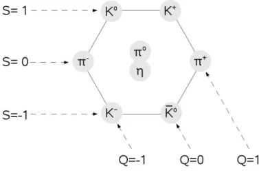
The η meson belongs to the ground state octet of pseudoscalar mesons as

shown in the fig. 1.1, with strangeness S = 0 and electrical charge Q = 0. The

η meson was discovered in pion-nucleon collisions at the Bevatron at Lawrence

Figure 1.1: The ground state pseudoscalar mesons octet in the coordinates of strangeness S along the vertical axis and electrical charge Q along the diagonal axis.

Berkeley National Laboratory in 1961 [4]. The basic properties of the η meson are listed in the table 1.3.

In terms of the quark model all mesons are quark-antiquark systems. There are nine qq combinations among u, d and s quarks and their antiquarks. The η meson is a linear combination of the octet η 8 and singlet η 1 states, given by the formula:

η = η 8 cos(θ) − η 1 sin(θ) (1.1) where octet η 8 and singlet η 1 states have quark composition given by formulas:

η 8 = 1

√ 6 (uu + dd − 2ss) (1.2)

η 1 = 1

√ 3 (uu + dd + ss) (1.3)

η = 1

√ 2 (uu + dd)cos(α) − ss sin(α) (1.4) The mixing angle θ was estimated in the range − (13.83 ^◦ − 18.76 ^◦ ), from the analysis of various decays of vector and pseudoscalar mesons, see [5], [6]. The mixing angle α is related to θ: α = θ + 54.7 ^◦ , see [7].

Recent measurements by CLEO-c [8] and KLOE [9] have confirmed the NA48

[10] value for η meson mass and nowadays the mass of the η meson is known with

a good precision. However, many rare decays of η were not measured precisely

because of lack of large statistics η samples. The η meson can participate in the

weak, strong and electromagnetic interaction. This and a relatively large mass

Table 1.3: The basic properties of the η meson, where B - baryon number, L - lepton number, S - strangeness, Q - electrical charge, isospin - I, J - spin, P - parity, C - charge conjugation and G - G-parity.

cause the η meson to have many decay modes [7]. An overview of η decay physics is given in [11, 12]. However, all decay modes via the strong, electromagnetic and weak interaction are forbidden in the lowest order, which explains why the η, with a life time of 5 × 10 ^{− 19} s, is relatively long lived particle. The positive eigenvalue for η charge conjugation (C) implies that decays into an odd number of photons are forbidden since the photon C eigenvalue is negative. Thus, also the very rare η → π ⁰ e ⁺ e ⁻ decay is forbidden if the electron-positron pair comes from a virtual photon. The decays into lepton-antilepton pairs η → µ ⁺ µ ⁻ and η → e ⁺ e ⁻ cannot proceed via a single virtual photon intermediate state since the spins of an η meson and γ differ by one unit. Within the framework of the Standard Model the decays which are dominated by a two virtual photon intermediate state are suppressed by helicity factors m l /m η at each γl ⁺ l ⁻ vertex. Thus the rates of these decays are small and they might be sensitive to hypothetical interactions.

Many η decays are forbidden by P , CP symmetries, for example the hadronic decays η → π ⁰ π ⁰ and η → π ⁺ π ⁻ . The non-hadronic decay modes are summa- rized in the table 1.4.

1.2 Transition Form Factors

The text below is partly taken from [14]. Electromagnetic structure of charged

particle can be obtained by scattering of the charged point-like probe on it. The

modification of the differential cross section by the charge distribution in the ob-

ject of study is given by:

dσ

dq ² = dσ

dq ² _point | F (q ² ) | ² (1.5)

where _dq ^dσ 2

point is the differential cross section for the scattering of an electron by a point-like charged particle, based on the predictions from Quantum Electro- dynamics (QED). The form factor F (q ² ) in 1.5 characterizes the spatial charge distribution in the particle and can be determined by comparing experimental re- sults on the differential cross section with the exact calculation for point-like par- ticle. In the non-relativistic case the form factor is related to the charge density distribution, described by a Fourier transformation.

The spatial structure of neutral mesons cannot be studied in a similar way because the process with single photon exchange is forbidden due to C - par- ity, conserved in strong and electromagnetic interactions, see table 1.1. Thus the electromagnetic form factors of neutral mesons are always zero and the internal structure of neutral mesons can manifest itself in radiative decays into a photon and meson of opposite C - parity: P → V γ. The photon can be real or virtual, in the latter case the virtual photon decays into a lepton pair l ⁺ l ⁻ , that is called internal conversion:

P → V γ ^∗ → V l ⁺ l ⁻ (1.6)

The invariant mass of the lepton pair equals to the four-momentum of the vir- tual photon. The lepton invariant mass distribution depends on the electromagnetic structure at the P → V transition vertex, which is due to a cloud of virtual states.

The dynamics of this mechanism is described by the transition form factor - the function of the four-momentum of the virtual photon. More details can be found in [14].

The vector meson V in the 1.6 can be replaced by a photon, in this case the decay is called single Dalitz decay: P → γγ ^∗ → γl ⁺ l ⁻ . The lepton pair mass spectrum is given by formula:

dΓ

dq ² = dΓ

dq ² _point | F P V (γ) (q ² ) | ² (1.7) The electromagnetic properties of the decaying meson P can be studied at P γ vertex. The transition form factor F P V (γ) (q ² ) in the 1.7 can be calculated from QED and normalized to the two photon decay width. Then the lepton pair mass spectrum is obtained:

dΓ(l ⁺ l ⁻ γ)

dq ² Γ(γγ) = 2α em

3πm s

1 − 4m ² _l

q ² (1 + 2m ² _l q ² ) 1

q ² (1 − q ²

m ² _P ) ³ | F P (q ² ) | ² (1.8)

γγγγ < 2.8 × 10 ⁻⁴ 3 × 10 ⁽ − 12) [27]

γγγ < 1.6 × 10 ^{− 5}

µ ⁺ e ⁻ + µ ⁻ e ⁺ < 6 × 10 ⁻⁶ 0

Table 1.4: Non hadronic decay modes of the η meson. The range for the predicted branch- ing ratio is an estimate of the influence of the form factor taken from [21] and [23].

Three electromagnetic decays of the η: η → llγ, η → lll ^′ l ^′ , η → ll contain in- formation about the transition form factor which is parameterized by the function F (q ₁ ² , q ² ₂ , m ² _η ), describing the ηγγ vertex. Here q 1 , q 2 are the four-momenta of the two photons. The transition form factor for single Dalitz decay F (q ² ₁ , 0, m ² _η ) has been measured fairly well for the decay η → γµ ⁺ µ ⁻ in [16], also for an overview of the η decays see [17].

1.3 The Decay Mode η → e ⁺ e ⁻ e ⁺ e ⁻

The decay η → e ⁺ e ⁻ e ⁺ e ⁻ is closely related to the radiative decays: η → γγ, η → γπ ⁺ π ⁻ , η → γe ⁺ e ⁻ which are driven by the chiral anomaly of Quantum Chromodynamics. The η → e ⁺ e ⁻ e ⁺ e ⁻ is due to the triangle anomaly and up to one-loop order this can be represented by the Feynman diagram in fig. 1.2a.

The decays of the η meson with lepton pairs can be related to the corresponding radiative decays with one or two photons using Quantum Electrodynamics and by introducing the transition form factor F (q ² ₁ , q ₂ ² , m ² _η ). The decay proceeds via two virtual photons each converting to a lepton pair: γ ^∗ → e ⁺ e ⁻ . Within the Vector meson Dominance Model (VDM) the interaction between η meson and two virtual photons proceeds via two vector mesons in the intermediate state (ρ, ω for example), fig. 1.2b. In the final state this decay has four leptons or two dilepton pairs and is called double Dalitz decay [18]. The four-momentum q of the emitted virtual photon can vary between twice the lepton mass and the mass of the meson.

The main interest in the lepton pairs is the fact that their invariant mass (m e ⁺ e ⁻ )

η

γ * γ *

e+

e- e+

e- _η ^{ρ , ω}

ω ρ ,

γ *

γ *

e+

e- e+

e-

a) b)

Figure 1.2: The diagrams for η → e ⁺ e ⁻ e ⁺ e ⁻ decay: a) Quark loop: triangle anomaly and b) Vector meson Dominance Model: vector mesons mediate the interaction between the η and the virtual photons

is equal to the four momentum transfer squared (q ² ) in the process of virtual pho- ton emission: m e ⁺ e ⁻ = q ² . Thus, the four–momentum squared distribution of virtual photons becomes experimentally observable by internal conversion of the virtual photons to lepton–antilepton pairs. The invariant mass of the lepton pair is an experimental observable while the momentum of the virtual photon can not be measured.

Fig. 1.3 shows a two-dimensional distribution of momenta of two virtual pho- tons of the double Dalitz decay of the η meson. The surface shape will tell about the function which describes the momenta distribution of γ ^∗ . Thus, the η → γ ^∗ γ ^∗ → e ⁺ e ⁻ e ⁺ e ⁻ decay allows to measure the η meson transition form fac- tor as a function of the momentum-squared of the two photons F (q ₁ ² , q ² ₂ , m ² _η ) in the time–like region for four–momenta between twice the lepton mass and the mass of the η. The four–momentum distribution of the virtual photons depends on the electromagnetic structure at the η → γ ^∗ γ ^∗ transition vertex. The form fac- tor correspondingly contains then dynamic information about the electromagnetic structure of the decaying meson [14].

Using the transition form factor, the differential decay width is then modified to:

dΓ

dq ² = dΓ

dq ² _point | F (q ₁ ² , q ² ₂ , m ² _η ) | ² (1.9) where the spectrum of effective masses of the lepton pairs for point–like ob- jects, _dq ^dΓ 2

point can be calculated reliably from QED, and the transition form factor

)

, (GeV/c

q

0 0.05 0.1 0.15 0.2 0.25 0.3 0

Figure 1.3: Simulation: two-dimensional distribution of the momenta squared of two virtual photons from η → γ ^∗ γ ^∗ : q ₁ ² on the X-axis vs q ₂ ² on the Y-axis, F = f (q ₁ ² , q ² ₂ , m ² _η ) = 1 .

)

, (GeV/c

q

Figure 1.4: Momentum squared of one of the virtual photons from η → γ ^∗ γ ^∗ with F (q ² ) = 1 (black) and with a pole type form factor from equation 1.10 (blue).

can be obtained experimentally.

In the left part of equation 1.9 is a differential decay width modified by intro- ducing the structure of the region of interaction. In the right part there is a known cross section for point-like objects multiplied by transition form factor, which can be obtained experimentally. Including the form factor modifies the mass spectrum of lepton pairs, as can be seen in the fig. 1.4, where a pole type formula was used for the form factor:

F (q ² ₁ , q ₂ ² ) = Λ ⁴

(Λ ² − q ² ₁ )(Λ ² − q ₂ ² ) (1.10) which corresponds to the standard double vector meson dominance model.

For the parameter Λ a mass of 770 MeV/c ² close to the mass of the ρ meson was taken. The effect becomes significant for higher masses, where two curves diverge. The effects of different form factors in meson-photon-photon processes were investigated in 2001 by Johan Bijnens and Frederik Persson [25].

Based on Quantum Electrodynamics, with a transition form factor F (q ₁ ² , q ² ₂ ) = 1 already in 1967 Jarlskog and Pilkuhn [21] evaluated the ratio based on earlier calculations [22]:

R 1 = Γ η → e ⁺ e ⁻ e ⁺ e ⁻

Γ η → γγ

= 6.6 × 10 ⁻⁵ (1.11)

As can be seen from comparing equation 1.9 and 1.11, the decay η → e ⁺ e ⁻ e ⁺ e ⁻

can be related to the η → γγ decay by using Quantum Electrodynamics, where both photons are real and the transition form factor is normalized to unity at q 1 = 0, q 2 = 0 (because for real photons m γ = 0), it implies the region of in- teraction is a point-like:

F (0, 0, m ² _η ) = 1 (1.12) According to equation 1.11 the branching ratio is BR _η→e ⁺ e ⁻ e ⁺ e ⁻ = 2.59 × 10 ^{− 5} . The calculations in [22] were done within QED, neglecting a cross term χ _ll in the amplitude which originates from the exchange of identical leptons or antileptons in different pairs. Similar calculations were done in [24] neglecting form factor influence. The result for the branching ratio with consideration of the cross term χ _ll gives BR = 2.56 × 10 ⁻⁵ . Neglecting the cross term the branching ratio slightly changes BR = 2.41 × 10 ⁻⁵ . Other calculations of the branching ratio with the cross term χ _ll were presented in [25]. The neglection form factor result gives the branching ratio 2.52 × 10 ⁻⁵ . Including the form factor from the VDM, three different form factor were used and the branching ratio was found in the range (2.52 − 2.65) × 10 ^{− 5} . The most recent calculations were done in [26], for QED case without cross term χ _ll the branching ratio was found 2.55 × 10 ⁻⁵ , with cross term 2.54 × 10 ⁻⁵ . Introducing two different form factors from VDM gives the range for the branching ratio (2.54 − 2.67) × 10 ^{− 5} .

Thus, the results for the branching ratio based on QED agree rather well be- tween each other. As can be seen introducing the form factor increases the branch- ing ratio. In general the branching ratio for η → e ⁺ e ⁻ e ⁺ e ⁻ does not expose sig- nificantly either by introducing the form factor or the cross term χ _ll . The influence of the form factor on lepton pair invariant mass spectrum was demonstrated in the figure 1.4: the effect becomes larger for higher masses.

In the framework of the analysis presented in the thesis the form factor influ- ence was neglected.

1.4 Available Data

The decay η → e ⁺ e ⁻ e ⁺ e ⁻ has not been yet observed and the only experi- mental data offer an upper limit for its branching ratio. The theoretical predictions based on Quantum Electrodynamics give a branching ratio of 2.6 × 10 ⁻⁵ , [21].

The latest experimental limit on the η → e ⁺ e ⁻ e ⁺ e ⁻ branching ratio comes from the CMD-2 experiment [19] at the VEPP-2M e ⁺ e ⁻ collider. The upper limit for the branching ratio of the η → e ⁺ e ⁻ e ⁺ e ⁻ was measured to be 6.9 × 10 ⁻⁵ with a confidence level of 90%. WASA/CELSIUS found two event candidates of the η → e ⁺ e ⁻ e ⁺ e ⁻ with an upper limit of 9.7 × 10 ⁻⁵ .

In parallel with the WASA activity there are ongoing studies, performed by the

KLOE experiment at the DAFNE e ⁺ e ⁻ collider in Frascati [30], with one of the

to ChPT. However there are no experimental data to check this.

WASA was designed for studies of the decay products of light mesons, par- ticularly it was optimized for dilepton pair identification by introducing material and dimensions to reduce the probability of photon conversion, the details will be discussed later in chapter 2. As it was mentioned, the upper limit for the branch- ing ratio is the only experimental information and WASA/CELSIUS has already identified it. The measurements were based on a 2 × 10 ⁵ η-s sample and now using the upgraded facility, having abundant η-sample and known methods which were used by WASA/CELSIUS, it becomes possible to obtain a solid number for the branching ratio and later focus on the lepton mass spectra study.

In this thesis a statistically more significant η-sample is analysed with a similar

method to that used by WASA/CELSIUS, therefore it can be expected to produce

a solid number for the branching ratio with lower statistical error. The aim of this

thesis is to present η → e ⁺ e ⁻ e ⁺ e ⁻ event candidates with reasonable signal-to-

background ratio and to determine the branching ratio of the η → e ⁺ e ⁻ e ⁺ e ⁻ .

and a detector setup. The accelerator facility delivers a beam of particles which interacts with the target and the products of this interaction are registered by a sys- tem of detectors. Instead of a fixed target a second beam of particles coming from the opposite direction can be used, in this case the accelerator facility is called a collider.

The Wide Angle Shower Apparatus (WASA) was designed to study light me- son production in hadronic interactions and their decays. The mesons are produced in proton-proton and proton-deuteron interactions. Originally it was operated at the CELSIUS ¹ ring in Uppsala, Sweden, with proton beam momenta up to 2.1 GeV /c. In summer 2005 after the shutdown of CELSIUS the setup was trans- ported to COSY ² facility, Juelich, Germany, which offers higher beam momenta up to 3.7 GeV /c as well as polarized beams. This adds possibility to study other mesons than η such as η ^′ , ω, φ.

After the setup was transferred to Juelich, its components were inspected in the laboratories of the Nuclear Physics Institute. Certain modifications and upgrades were done in order to improve the detector performance. The data acquisition has been renewed.

The detector is operated with an internal hydrogen and deuteron target using a pellet target system with effective target densities > 10 ^{15 atoms} _cm 2 providing high luminosities in the order of 10 ³² cm ⁻² s ⁻¹ .

1 Cooling with Electrons and Storing Ions from Uppsala-cyclotron

2 COoler SYnchrotron

13

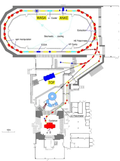
Figure 2.1: COSY floor plan: schematic view

296 GeV /c.

COSY has the shape of a longitudinally stretched ring with two arc sections of 52 m length and two straight sections of 40 m length, where the internal experi- ments are located. Comparing with the conditions at CELSIUS, COSY offers cer- tain improvements in experimental conditions: fast magnet ramping, dispersion- free target position, electron and stochastic cooling and a smooth microscopic time structure of the beam. The COSY ring can be filled up 10 ¹¹ particles lead- ing to typical luminosities of 10 ³¹ cm ⁻² s ⁻¹ with a cluster target and 10 ³² cm ⁻² s ⁻¹ with a pellet target. Two cooling systems [33] are used: electron-cooling at injec- tion energy and stochastic cooling for higher momenta. The electron cooling is used with 22 keV electrons to increase the intensity of the polarised proton beam.

Stochastic cooling is working in the proton momenta range between 1.5 GeV /c and 3.5 GeV /c.

After acceleration and injection, the beam is stored and can be used for exper- iment. In case of internal experiments, the beam interacts loses its intensity. Thus, the beam in the storage ring has only a certain lifetime. When it is used up, new particles have to be injected. The time between two injections is called a it cycle.

A typical beam cycle during the beamtime in November, 2008 is shown in the figure 2.2. The beam intensity is defined by the beam current and is decreasing to the end of the cycle due to interaction with the pellets, following the black curve.

2.2 Pellet Target

The study of rare processes puts some demands on the target: a suitable effec- tive target thickness (in the order of 2 × 10 ^{15 atoms} _cm 2 ), a good definition at the interac- tion point definition and access to a solid angle close to 4π. Another requirement is especially important for final states with electron-positron pairs - that there should be only little material for the reaction products to reach the detectors. This helps to minimize the background from photon conversion. All these requirements can be met with a pellet target.

The pellet-target system is an unique target developed particularly for high

Time in cycle, s

0 20 40 60 80 100 120

Arbitrary units

0 2000 4000 6000 8000 10000

BCT, arbitrary units Pellet rate, arbitrary units

Figure 2.2: Beam current in arbitrary units and pellet rate per second on the Y-axis as a function of time in cycle on the X-axis during a beamtime in November, 2008, reaction pp → ppη at 1.4 GeV . That illustrates how the beam intensity is decreasing due to beam- target interaction.

luminosity and high precision measurements [34]. The setup produces a narrow stream of frozen hydrogen droplets which cross the beam vertically from above.

The idea of using a running stream of droplets was first proposed in 1984 by Sven Kullander at CELSIUS.

The layout of the setup is depicted in figure 2.3. The pellet generator is located on top of the setup where a high purity jet of liquefied gas (H 2 , D 2 ) is broken up into individual droplets by vibrating glass nozzle. When the droplets enter the vacuum chamber through an injection capillary they freeze due to evaporation and become solid spheres or pellets. At the same time they are accelerated up to velocities of 100 m/s by the gas flow through the capillary. Further down a skim- mer is used to collimate the pellet beam before entering the pellet beam tube. The pellet tube is 2 m long and has a diameter of 7 mm. The pellets have a size of 20- 40 µm and form a pellet beam with a diameter of 2-4 mm at the interaction point.

The small size of the pellets is one of the important parameters to achieve a well defined interaction point and to reduce the probability of secondary interactions in the target.

The initial droplet rate is determined by the vibration frequency of the noz- zle. However, mainly due to turbulences during the vacuum injections the typical pellet rate is 3000-10000 s ⁻¹ after collimation at the interaction point. The typi- cal operation parameters of the pellet target are summarized in the table 2.1. The photo of the pellet stream is shown in the figure 2.4.

After passing the COSY beam the pellets are stopped in the pellet beam dump

and the gas from the evaporating pellets is removed by turbo pumps.

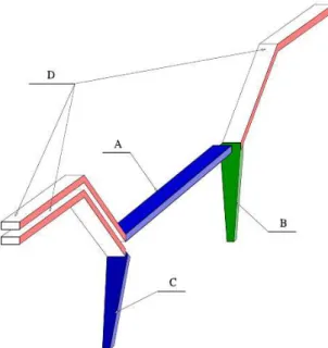
Figure 2.3: Pellet target setup: schematic view.

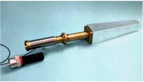
Figure 2.4: Photo of the pellet target stream: the nozzle (truncated cone) is at the top, the

vacuum capillary in the lower part.

Pellet size 20-40µm Pellet frequency

at nozzle 70 kHz

at interaction point 5-12 kHz Pellet flight velocity 60-100 m/s Pellet beam angular divergence 0.04 ^◦

Table 2.1: Typical pellet target parameters achieved during the beamtime in October- November, 2008.

2.3 WASA Detector

The WASA detector was designed to study the decays of light mesons. It can be divided into two main parts, the forward and the central detector. The forward detector provides the reconstruction of the recoil particles and allows to tag on the produced meson via the missing mass technique. The central detector then detects and identifies both charged and neutral decay products of mesons.

A cross section of the complete setup is shown in the figure 2.5. The WASA master coordinates x, y, z are given in a right handed coordinate system with the origin at the vertex of the reaction. The z-axis is directed along the beam, the x-axis goes perpendicular to the z-axis outward from the COSY ring in the hori- zontal plane, the y-axis is orthogonal to x-z plane directed upwards.

In the following sections the individual components of the detector are de- scribed in more details.

2.3.1 Central Detector

The central detector measures charged particles and photons originating from meson decays. The Mini Drift Chamber (MDC) and the Plastic Scintillator Barrel (PSB) are placed inside a magnetic field provided by a superconducting solenoid.

With the MDC the momenta of charged particles are measured and positively and negatively charged particles are distinguished by the bending direction of the track in the magnetic field. The PSB also delivers information about the energy deposit of charged particles and provides fast signals which are used on trigger level.

In addition the Scintillator Electromagnetic Calorimeter (SEC) surrounds MDC and PSB and measures the energy deposit of both charged and neutral particles.

In combination with the information from the PSB one can distinguish between charged and neutral particles.

The Central Detector covers polar angles in the range from 20 ^◦ to 169 ^◦ and

the complete azimuthal angular range. All three components together provide the

Figure 2.5: Cross section of the WASA detector. For a discussion of the individual com- ponents see text.

full four-momentum for each particle.

2.3.1.1 Mini Drift Chamber

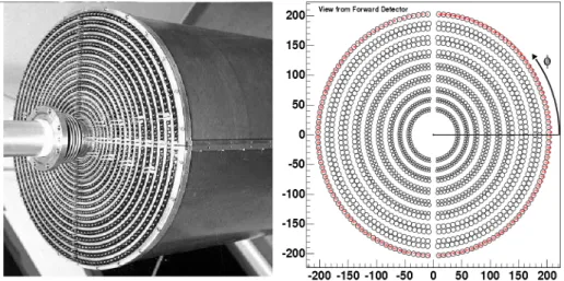
The MDC is used to measure charged particles. It is built around the interac- tion point covering scattering angles from 24 ^◦ to 159 ^◦ . The detector consists of 1738 drift tubes in a cylindrical geometry. The tubes are organized into 17 con- centric layers centered at the beam axis. In order to keep the amount of material low and to reduce secondary interactions, each tube is made from a thin 25 µm aluminized mylar wall tube and a stainless steel sensitive wire of 20 µm diameter.

These type of drift tubes is called straw tube .

The mechanical construction of the MDC is symmetric with respect to the

Y Z − plane and can be divided into two halves: each layer of the MDC consists of

two semi-layers, which form a cylindrical surface. The most inner and outer layer

of the straw tubes are located in radii of 41 and 203 mm respectively. Numbering

the layers from inside to outside, the nine odd layers are parallel to the z − axis

while the eight even layers are stereo layers with different skew angles (6 ^◦ − 9 ^◦ )

with respect to the z − axis. Therefore, the axes of the tubes in stereo layer form

a hyperboloidal surface. The axial layers provide two-dimensional information

about the track coordinates in the XY -plane. In addition, the stereo layers are

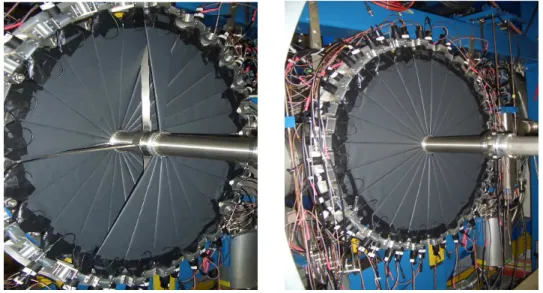
Figure 2.6: Left: backward photo of the MDC layers with incoming beam pipe. Right:

depiction of the straw tubes as a projection to XY-plane, the scale on the axes is in mil- limeters.

used to measure the z coordinates of the track.

The layers can be divided into three groups with diameters of 4, 6 and 8 mm.

The first five inner layers have a diameter of 4 mm. Furthermore, the length of these tubes is increasing from inside to outside due to the cone shape of the scat- tering chamber in forward direction (see the black contour in the figure 2.5). The outer most twelve layers have the same length: the layers from six to twelve have a diameter of 6 mm, the five outer layers have a diameter of 8 mm. All layers are aligned with respect to the backward end of the MDC, see figure 2.6, left. Each layer is supported by Al − Be (50%Al-50%Be) semi-cylindrical plates, i.e. semir- ings, see figure 2.7. These semirings are interleaved with the straw tube layers and finally the whole construction is covered by a 1 mm thick Al − Be cylinder. Each semi-layer can be flushed with gas individually. The semi-layers were joined into one layer which is flushed with gas. Thus, each MDC layer is monitored by means of input and output gas flows. During the inspection of the MDC before the instal- lation at COSY gas leakages were identified and classified by the gas losses.

The MDC is operated with a commonly used gas mixture: 80 %Ar and 20

% C ₂ H ₆ at atmospheric pressure. This choice of the gas mixture has several ad-

vantages: relatively low operating voltage can be applied to the wires in order to

provide a high rate capacity and, therefore, the operation becomes more safe, as

the major component of the mixture is noble gas the low interaction ability of gas

with material of straws prevents from aging effects [35]. Another advantage is the

linear drift function of the gas mixture. Additional information can be found in

[31].

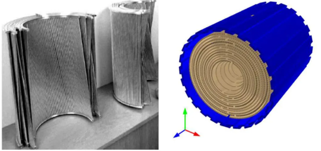
Figure 2.7: Left: the semi-cylindrical plates support and separate the layers of straw tubes, the visible inclined plate illustrates how the stereo layers are interleaved with the parallel layers. Right: barrel part of the PSB(blue) covers the MDC layers.

Signal wires are connected to newly developed electronics based on CMP-16 amplifier-discriminators (for details see [36] ) via combined signal-high voltage cables. The CMP-16 modules produce a logic signal in the LVDS-standard ³ which is then passed to a TDC ⁴ .

The working principle of the MDC is based on the motion of charged particles in an electric field: when a charged particle crosses a gas volume the gas is ionized and the produced electrons are accelerated along the electric field, finally produc- ing an electron avalanche and positively charged ions in the region close to the anode-wire. The information about the coordinates of the charged particle track is determined through the measurement of the drift time of electrons and ions, more detailed information can be found in [37]. The chamber measures three di- mensional trajectory of a charged particle in a nearly uniform magnetic field, then the momentum is calculated from the curvature of particle trajectory in magnetic field.

The momenta of electrons and positrons can be measured in the range about of 20 M eV /c - 600 M eV /c. The momentum range of heavier charged particles are slight different, for pions the range is 100 M eV /c - 600 M eV /c, for protons it’s 200 MeV/c - 800 MeV/c.

The MDC performance during the beamtime in spring 2008 is shown in the figure 2.8. This study is based on the reaction pp → dπ ⁺ at 600 M eV , where the π ⁺ is identified in the Central Detector by PSB and SEC and the deuteron is

3 Low Voltage Differential Signal

4 Time-to-Digital Converter

2 4 6 8 10 12 14 16 10

20 30 40 50 60 70 80 90 100

Layer efficiency, %

Figure 2.8: The MDC layer efficiency based on the tracks reconstructed by the PSB and SEC. The lower efficiencies of the first layers are due to larger amount of not responding channels, the fifth layer has the largest number of 20% damaged tubes from total number of tubes in the layer.

detected in the Forward Detector. The signature of the two body reaction allows the preselection of a clean sample of one track events in the Central Detector. The histogram illustrates the individual layer efficiencies of the MDC, which are based on the amount of MDC tracks relatively to the tracks found by PSB and SEC. The average efficiency is around 80 % for individual layers.

2.3.1.2 Plastic Scintillator Barrel

The Plastic Scintillator Barrel (PSB) surrounds the mini drift chamber and consists of three parts: the central (barrel) part and forward and backward end caps, see figure 2.9. The central part has a cylindrical geometry around the beam axis. Each part is made of 48 thin plastic elements of 8 mm thickness, see figure 2.3.1.2. The most bottom and the most top elements in the barrel are divided into two halves in order to provide space for the pellet target pipe: the gaps are visible in the figure 2.9.

The elements in the barrel overlap by 6 mm. With such design gaps between

two neighboring strips can be avoided and resulting in an increased detection effi-

ciency. The forward and backward parts consist of elements of trapezoidal shape,

see figure 2.9. The elements in the forward cap are perpendicular to the beam axis

Figure 2.9: From left to right: forward, central and backward part of the PSB. Two holes situated diametrically opposite in the central part are for pellet target pipes.

and flat, forming a disc. The elements in the rear cap are inclined outward and form a conical surface with an angle of 60 ^◦ . Each element is read out individually by a photomultiplier. The scintillation light is transferred from the scintillator to the photomultiplier via light guides.

The PSB provides time and amplitude information and has two important functions:

• as a thin plastic scintillator it provides fast time signals for the trigger logic discriminating charged and neutral particles

• the energy deposit is used for particle identification via ∆E-p plots.

2.3.1.3 Superconducting Solenoid

The Superconducting Solenoid (SCS) surrounds MDC and PSB and provides an axial magnetic field along the Z -axis. The thickness of the solenoid is opti- mized such, that photon conversion is minimized. Accuracy of the energy mea- surements in the calorimeter and equals to 0.18 X 0 . The coil is cooled down by liquid helium and operated at 4.5K.

The return path for the magnetic flux is provided by an iron yoke, the red thick

contour in figure 2.5. The yoke has two purposes: it confines the magnetic field in

the central part of WASA and serves as support structure for the photomultipliers

of the calorimeter. It contains 1012 holes for connecting the calorimeter crystals

to their photomultiplier tubes by means of plastic light guides. The magnetic field

was measured by a hall probe. The field distribution was calculated and compared

with simulations of magnetic field distributions. The distribution of the magnetic

field inside the iron yoke calculated for a coil current of 667 A is shown in the

Figure 2.10: Schematic view of one Plastic Scintillator Barrel element: from forward part (B), central part (A) and backward part (C). The light is transferred by lightguides (D).

figure 2.11. The field uniformity inside the MDC is 1.22 ± 20% T. A more detailed description of the SCS can be found in [38].

2.3.1.4 Scintillating Electromagnetic Calorimeter

The Scintillating Electromagnetic Calorimeter (SEC) is placed between the solenoid and the iron yoke, covering the MDC and the PSB. It consists of 1012 sodium doped CsI crystals for measuring energies and angles of photons and charged particles in the polar angular range between 20 ^◦ and 169 ^◦ .

The SEC is divided into three parts: the central part and two end caps (back- ward and forward), see figure 2.12. There are gaps between the central part and end caps which are needed for the lightguides of the Plastic Scintillator Barrel.

It covers nearly the complete azimuthal angle from 0 ^◦ to 360 ^◦ having two holes for the pellet pipe and the solenoid chimney for liquid helium (not shown in the figures).

Each crystal has a shape of truncated quadrangular pyramid (figure 2.13). The

crystals are organized into 24 rings (layers) with centers situated on the beam

pipe axis. The forward end cap is represented by 4 layers of 36 crystals each and

covers the scattering angle in the range an 20 ^◦ -36 ^◦ . The central part consists of 17

Figure 2.11: Calculated values of the magnetic field inside the iron yoke for a coil current of 667 A. The marked contours constrain the regions with the same magnetic filed values.

Contour maxima are indicated by lines marked A-H, where: A =0.10 T, B=0.25 T, C=0.50 T, D=0.75 T, E=1.00 T, F=1.20 T, G=1.30 T and H=1.50 T.s

layers with 48 crystals each, covering an angular range 40 ^◦ -140 ^◦ and the backward end cap (red elements in the left part of the figure 2.12) with 3 layers of crystals covers the angles up to 169 ^◦ . More detailed information about the mechanical construction of the SEC can be found in [39], [40].

The placement of the solenoid inside of the calorimeter allow using photomul- tipliers outside of the return yoke. Lightguides are used for signal transmission from the crystals to the photomultipliers through the iron yoke, see 2.13. Thus, all read out electronics is situated outside the magnetic field and not affected by that. The SEC is involved in the trigger logic by using the information about the multiplicity of groups of crystals above a variable energy threshold.

The minimum energy for photon detection in SEC is around 2 MeV. The rel- ative energy resolution for photons is given by: ^σ _E ^E = ^{√ 5%} _E , where the energy E is measured in GeV . The angular resolution is limited by the crystal size.

2.3.2 Forward detector

The forward detector measures charged recoil particles and scattered projec-

tiles in the polar angular range between 3 ^◦ and 18 ^◦ . It consists of 11 scintillator

hodoscopes in different configurations and 4 planes of straw tubes. The subdetec-

tors form a sequence of planes each one perpendicular to the beam axis except the

first layer of the Forward Window Counter. This resembles the conical surface of

the exit window of the scattering chamber, see 2.5.

Figure 2.12: Left: the view cut of the Scintillating Electromagnetic Calorimeter, crystals of the backward part are marked red, crystals of the forward part are marked green, the central part crystals are white. Right: the coverage of the polar angle by the calorimeter.

The numbers on the top correspond to the numbers of crystals per calorimeter ring.

Figure 2.13: Fully equipped calorimeter module with CsI crystal, lightguide, photomul-

tiplier and housing.

Figure 2.14: The photo of the FWC. Left: a complete first layer and some segments of the second layer. Right: complete second layer overcasts the first layer.

In general, time and amplitude information from the scintillators is used in the trigger logic and later for particle identification by using the ∆E-E technique. The straw tube detector is used to improve the angular resolution by measuring precise track coordinates.

In the next subsections the geometry and the purpose of each component of the forward detector is given.

2.3.2.1 Forward Window Counter

The Forward Window Counter is the first subdetector following the exit win- dow of the scattering chamber. It consists of two layers of scintillator counters in a pizza-like shape. Both layers are made from 3 mm thick plastic scintillators.

Each layer consists of 24 radial segments which are read out individually by pho- tomultipliers. The layers are shifted by half of segment respectively to each other providing overlap between scintillators and, therefore, a complete coverage in az- imuthal angle. The first layer is inclined by 80 ^◦ respectively to the beam axis and adheres closely to the scattering chamber surface, forming a conical surface. The second layer is planar, perpendicular to the beam axis and is situated right after the first layer, see figure 2.14.

Using this detector in the trigger significantly reduces the background from

secondary interactions in the beam pipe. A low and high threshold on the ampli-

tude allows the discrimination of particles according to their ionization density.

This is used to separate ³ He tracks from the protons and deuterons, since ³ He ions deposit more energy than protons and deuterons. Thus, it provides cleaner tagging of the pd → ³ Heη reaction already on trigger level.

2.3.2.2 Forward Proportional Chamber

The Forward Proportional Chamber (FPC) is placed directly after the Window Counter. It consists of 4 planar modules, each with four layers of 122 cylindrical drift tubes (straw tubes) of 8 mm diameter. Similar to MDC, see 2.3.1.1, the tubes are made from aluminized mylar of 26 µm thickness. The sensitive wire is made from stainless steel and has a diameter of 20 µm. Each wire is stretched with a tension of 40 g.

The straw tubes in the layers are staggered by shift of one tube radius respec- tively each other. This is the most dense configuration, providing as much as many tubes as possible along the straight trajectory of the particle. The first two mod- ules are rotated by -45 ^◦ and +45 ^◦ degrees in azimuthal angle, see figure 2.15. The tubes in the third module are parallel to Y − axis and in the last, fourth, module the tubes are parallel to X − axis. Similar to MDC, the straw tubes of the FPC are read out from one side by the same electronics, however different to the MDC the electronics is mounted directly on the modules, avoiding signal transmission via the high voltage-signal cables.

The FPC is supplied by a common gas system for straw detectors, providing 20%C ₂ H ₆ -80%Ar gas mixture under atmospheric pressure. In September 2007 all four modules were installed and operated all together the first time. The FPC serves as an accurate coordinate detector providing precise angular information for reconstructing tracks of the particles originating from the target region.

2.3.2.3 Forward Trigger Hodoscope

The Forward Trigger Hodoscope is the next scintillator detector placed after the FWC. It is built from three layers of 5 mm thick plastic scintillators. The first layer counts 48 sectors in a pizza-like manner. The two others layers consist of 24 elements each, built as Archemedian spirals with different orientation to each other. Such a special geometry provides a pixel structure.

In figure 2.16 the situation with two charged tracks crossing the FTH elements is shown (fired elements are marked black). In the right panel the projection of the layers illustrates how two tracks cross them, each point is defined by the elements from three layers. With this structure it is possible to solve multi-hit ambiguities.

All elements are read out individually by photomultipliers.

The FTH plays an important role in the trigger logic. It provides hit multiplic-

ity as well as azimuthal and polar angular information on the trigger level.

Figure 2.15: The FPC modules: 3-D view to the left and the position of the tubes in different modules to the right(some internal tubes are removed for better illustration).

Figure 2.16: The FTH view, left is a 3-D view of element orientation in each layer; right

is a projection of elements from all layers.

Figure 2.17: The FRH layers are situated behind each other, the dimensions are in mm.

2.3.2.4 Forward Range Hodoscope

The Forward Range Hodoscope (FRH) is a system of five layers of thick plas- tic scintillators: the first three layers have a thickness of 110 mm thickness, the other two of 150 mm. Each layer is a disc with 24 plastic scintillators, arranged in a pizza-like manner. The diameter of every next layer is increasing, in order to cover the full angular range up to 18 ^◦ . The fifth layer diameter is the same as the fourth, see figure 2.17.

The main purpose of thick detector is to measure the energy loss of the parti- cles, which will then be used to recalculate the initial kinetic energy at the interac- tion point. The stopping power of the Range Hodoscope for pions is 200 M eV , for protons 360 M eV , for deuterons 450 M eV , ³ He ions 1000 M eV can be stopped and α-particles 1100 M eV . As a scintillator detector the Range Hodoscope pro- vides fast signals to the trigger logic.

2.3.2.5 Forward Range Intermediate Hodoscope

The Forward Range Intermediate hodoscope is a double layer hodoscope placed

between the second and the third planes of the FRH. There are 32 rectangular ele-

ments in each layer, in the first layer the elements are situated horizontally and in

the second - vertically, see figure 2.18. This is an additional scintillating detector

Figure 2.18: The FRI hodoscope:

two layers of scintillators perpendic- ular to each other.

Figure 2.19: The FVH hodoscope:

one layer of scintillators.

for a position measurements inside the FRH, it helps to suppress secondary inter- actions inside the FRH material. More detailed information about the FRI can be found in [42].

2.3.2.6 Forward Veto Hodoscope

The Forward Veto Hodoscope is the last active component in the FD. This is one layer of twelve horizontally oriented rectangular plastic scintillators. Each scintillator is a 20 mm thick and 137 mm wide. The Forward Veto Hodoscope (FVH) is drawn in the figure 2.19. The scintillators are read out from both ends by photomultipliers. The FVH is used in the trigger logic for the registration of punch-through particles and identification of certain undesired reactions.

2.3.2.7 Forward Range Absorber

The Forward Range Absorber is a passive component, placed between the FRH and the FVH. It is made from 5 mm thick iron plates which can be put to- gether and provide a total thickness of 100 mm. The Forward Range Absorber(FRA) is equipped with supporting rails and can be easily moved in or out.

The FRA was designed to stop slow protons from η-production in proton elas-

tic scattering reactions. Fast protons penetrate the FRA and trigger signals in the

FVH which can be used for veto in the trigger system.

2.3.3 The light-pulser monitoring system

The light-pulser monitoring system is used for monitoring all photomultipliers in the whole detector. The light pulser provides a reference light pulse for each photomultiplier, which can be used for monitoring its stability. There are two types of light sources: one "slow" source for monitoring of the photomultipliers of the calorimeter and four "fast" LED-based sources for the photomultipliers of the plastic scintillators.

The light pulser monitors the stability of the scintillation counters with a pre- cision ∼ 1 %, which corresponds to the energy resolution for stopped particles.

The system has the possibility to change the intensity of light flashes that also al- lows to study the calibration and linearity of the detectors. A detailed information about the light-pulser monitoring system can be found in [43].

2.4 Data Acquisition system

The Data Acquisition system (DAQ) is a set of electronic devices that orga- nizes the process of handling and storing of measured variables as digital infor- mation.

The DAQ, currently used at WASA, belongs to the third generation of the DAQs developed by Central Institute for Electronics (ZEL) at COSY. It is able to provide a read-out with short dead-times in the order of 20-30µs and, thus, allows the WASA detector to run at high luminosities and high event rates. For details see [44].

An overview of the DAQ system developed for WASA is shown in figure 2.20.

The analog signals from the detectors are processed through the preamplifiers, dis- criminators and splitters and transformed into digital signals by TDCs and QDCs ⁵ . TDCs and QDCs are continuously digitizing and storing the signals in internal buffer. This allows trigger delays up to 2µs and avoids delaying the data signals.

The plastic scintillators provide both time and amplitude information and are read out by TDC and QDC modules. The straw tube detectors provide time informa- tion only and are read out by TDC modules. The TDC and QDC modules are organized in LVDS crates, each crate is equipped with a system controller for the communication between the crates and the readout computer farm, see figure 2.20.

All data are collected by an event builder and finally stored on disc. The design of the DAQ allows data rates of ≈ 80 M B/s.

5 Time- or Charge-to-Digital Converter

Figure 2.20: The scheme of the DAQ.

2.5 Trigger system

The goal of the trigger system is to reduce the initial amount of events by se- lecting those that satisfies the experimental interests. The trigger system of WASA is drawn schematically in figure 2.21. In general, the triggers can be divided into fast and slow triggers. Fast triggers are produced by the plastic scintillators from all over the setup. This type of trigger is based on hit multiplicities of detector layers, their coincidences, cluster multiplicities and track alignment in the forward detector. The slow triggers use the information from the SEC: cluster multiplicity and energy deposits in the crystals (e.g. so-called energy-sum trigger).

Following the scheme in the figure 2.21, the multiplicity signals are matched

and than combined into more complex trigger expressions. Depending on the fre-

quency of the triggers they can be prescaled in order to balance the event rate.

Figure 2.21: The schematic drawing of the trigger system.

programming. The sketch of the data analysis chain is depicted in figure 3.1.

Following the scheme from the top, there are two possible inputs for Root- Sorter: experimental data as they come from the data acquisition and simulation.

In case of simulations the desired reactions are generated using the event generator Pluto. Then the generated events are tracked through the detector setup, described by a GEANT3 based on Monte Carlo simulations.

Simulations are always necessary for evaluation of experimental data. The study of the rare processes requires large event samples in order to develop the analysis methods by considering the kinematics of the process and the detector response.

This chapter will cover the tools that were used for simulation and for data analysis, as well as the calibration procedures for the central detector compo- nents, focusing on the Mini Drift Chamber. In addition the track reconstruction in both parts of the WASA setup will be discussed. The relevant plots of the particle identification are shown for pd → ³ Heη at 1 GeV .

3.1 Software Tools

3.1.1 Event Generator Pluto++

An event generator is used to get correctly determined sets of Lorentz-vectors for a given physics reaction. Pluto is an event generator entirely based on the ROOT software package and designed for hadronic interactions like meson pro-

35

Figure 3.1: Schematic drawing of the data analysis chain.

Γ ^{A →2γ} dm =

3πm 1 − m ^{2 e} (1 + ^e

m ² )(1 − m ² _A ) | F A (m ² ) | ² (3.1) Formula 3.1 describes the mass sampling for virtual photons, where index A refers to the parent meson (e.g. η), m is the dilepton mass, m e is the electron mass and m A is the meson mass. The last factor is the parent form factor. In the first approach for η meson this form factor was taken as one-pole approximation:

F A (m ² ) = 1 1 − ^m Λ ^{2 2}

(3.2) where Λ = 0.75 GeV is used according to Vector-Meson-Dominance-Model calculations. Experimental measurements yield Λ = 0.72 ± 0.09 GeV based on the single Dalitz decay η → µ ⁺ µ ⁻ γ , [29]. Both results from theory and experiment indicate that the interaction between mesons and virtual photons proceeds via an intermediate ρ-meson.

Similarly, the double Dalitz decay of the η meson can be generated. In this work, the influence of the form factor was neglected: F A (m ² ) = 1, because of the poor statistics of the experimental data. As it was shown in figure 1.4 the form factor influences the region of high lepton pair masses, while in the region of low lepton pair masses the influence is small. The interference between lep- tons, discussed in 1.3 is not considered either. In this work, the simulation of the background channels was performed using the Pluto version 5.31.

3.1.2 Detector Simulation Monte Carlo Package

The simulation of the WASA detector is done with a Monte Carlo package, based on the GEANT3 software [47]. The main purpose of the Monte Carlo soft- ware package is the study of the detector response for different physical processes.

The simulation tool reproduces the properties of the experimental setup as close

as possible to reality including the construction of the setup, the material proper-

ties of the detector components together with the supporting mechanics and parti-

cle interaction with the detector material. Additional effects are implemented via