Pion Structure from Lattice QCD

(1)

Pion Structure from Lattice QCD

Dissertation

zur Erlangung des Doktorgrades der Naturwissenschaften (Dr. rer. nat.)

der Fakultät für Physisk der Universität Regensburg

vorgelegt von

Narjes Javadi Motaghi

aus Arak, Iran

im Jahr 2015

(2)

pr¨ufungsausschuss: Vorsitzender: Prof. Dr. C. Strunk 1. Gutachter: Prof. Dr. G. Bali 2. Gutachter: Prof. Dr. V. Braun weitere Pr¨ufer: Prof. Dr. F. Evers Termin Promotionskolloquium: 12.05.2015

(3)

I dedicate this thesis to my beloved parents

(4)

(5)

Preface

The history of elementary particle physics is around 100 years old. Elementary particle physics was born in 1897 with the discovery of the first elementary particle, the electron, by J.J.Thomson¹. The electron was and still is considered as an elementary particle which means a point-like particle with no inner structure. In contrast to the electron, atoms have an inner structure which was first shown by Rutherford’s gold foil experiment in 1911 [Rut11]. It showed that each atom consists of a nucleus which contains most of the atom’s mass and it is surrounded by a cloud of electrons.

Until 1918 the proton was the only other known elementary particle. Later, in the early 30s another particle named neutron was discovered which was slightly heavier than the proton but carried no charge. The nature of the force which keeps the nucleus together was yet missing. Though, it was clear it must be a very strong force, only attractive for protons and neutrons with very short range, and therefore not noticeable in everyday life.

In 1935 a new field was predicted by Hideki Yukawa. He proposed the existence of an exchange particle for the strong force which should have the mass of nearly 300 times that of the electron, but about a sixth lighter than the proton. He called it meson (middle–weight) which should be responsible for the exchange of the strong force between protons and neutrons. However, no such particle had been observed in the laboratory before.

At that time a number of cosmic rays studies were in progress, and in 1937 two different groups identified a particle matching Yukawa’s description. But the observed cosmic ray particle had a wrong lifetime and interacted very weakly with the atomic nucleus. Moreover, it was significantly lighter than expected from Yukawa’s prediction. This puzzle was resolved in 1947 by physicists at Bristol University in England.

They discovered the existence of two middle–weight particles in cosmic rays, which are known today as thepion π and muon µ. The pion was identified as the true Yukawa meson. Simultaneously, the same conclusion on theoretical grounds was reached by Marshak [MB47]. Pions are produced in huge numbers when cosmic rays bombard the earth and collide with atoms in the upper atmosphere. These pions ordinarily decay long before reaching the ground and the Bristol group therefore had to display their photographic emulsions on mountain tops. Later, particle physics experiments showed

1We follow the lecture notes of [Fra02] and chapters 1 and 2 [Gri08] and references therein.

(10)

theµ does not participate in the strong nuclear interaction and nowadays it classified as a lepton and not a meson.

The existence of pions as charged particles was identified by their double traces on photographic plates. Charged pions decay to a muon and a neutrino (or anti-neutrino)

π⁻→µ⁻+ ¯ν_µ, (1.0.1)

π⁺→µ⁺+ν_µ. (1.0.2)

The branching ratio² says that the probability for the decayπ⁺⁽⁻⁾→µ⁺⁽⁻⁾+ν_µ(¯ν_µ) is larger than that forπ⁺⁽⁻⁾→e⁺⁽⁻⁾+νe(¯νe). Besides the charged pions, there is also a chargeless one, theπ⁰, which does not leave traces in photographic plates. The neutral meson was therefore discovered later in 1950. Aπ⁰ decays as

π⁰→e⁻+e⁺+γ. (1.0.3)

The neutral pion has lifetime of about 10⁻¹⁶ seconds, whereas the charged ones have longer lifetimes of about 2.6×10⁻⁸s. A π⁰ is π⁰ = 1/√

2|u¯u−ddi¯ and the charged pions are made of a pair of quark anti-quark, each (π⁻ = |d¯ui, π⁺ = |udi). The¯ neutral pion is slightly lighter than charged pions, m_π^± = 139.57 MeV and m_π⁰ = 134.97 MeV [B⁺12, O⁺14]. The deviation between masses can be due to the electromagnetic self-energy [D⁺67]. The strong interaction properties of the three pions are identical.

The Nobel Prizes in Physics were awarded to Yukawa in 1949 for his theoretical prediction of the existence of pions, and to Cecil Powell in 1950 for developing and applying the technique of particle detection using photographic emulsions.

Besides pions and muons, many other particles have been discovered in the 40’s and 50’s by operating the new high energy accelerators, as Willis Lamb humorously pointed out in his Nobel prize acceptance speech: “When the Nobel prizes were first awarded in 1901, physicists knew something of just two objects which are now called elementary particles: the electron and the proton. A deluge of other elementary particles appeared after 1930; neutron, neutrino,µmeson,π meson, heavier mesons and various hyperons. I have heard it said that the finder of a new elementary particle used to be rewarded by a Nobel Prize, but such a discovery now ought to be punished by a$10,000 fine [Gri08, pn55]”. The particle zoo began to fill including elementary particles and also composite ones, like hadrons. However, at that time it was yet unclear which one was elementary and which was not.

A first successful attempt to introduce some structure into the particle zoo was done by Gell-Mann and independently by Zweig in 1964 [GM64, Zwe64]. They introduced that hadrons consist of elementary constituents called quarks. In the original quark model, quarks came in three flavors up, down and strange, but later until 1983 other three quarks charm, top and bottom were discovered [Ros81]. Quarks are elementary

2There are severals ways for a particle to decay. The probability of its decay to a particular mode is known as its branching ratio for that decay mode.

(11)

particles with spin 1/2 and fractional electric charge flavor charge u c t +²₃e d s b −¹₃e

(1.0.4)

Initially, there had been many doubts on the real existence of quarks as the inner constituents of hadrons. But this was eventually proven by some experiments like deep inelastic scattering (DIS) experiments at the Stanford Linear Accelerator Center (SLAC) in 1968 [B⁺69].

The quark model was successful in classifying hadrons as bound states of quarks but at the same time another problem appeared: the existence of a hadron consisting of three up quarks with parallel spin ∆⁺⁺ [Bru52]. It showed that quarks have to have a further quantum number, otherwise these states would violate Pauli’s exclusion principle. It says that no two particles with half integer spin can occupy the same state.

The puzzle was solved by O. W. Greenberg [Gre64]. He proposed that quarks come not only in three flavors but each of them also comes in three color charges commonly named red,green and blue. These color charges have nothing to do with visible colors of light in everyday life. All observed hadrons are colorless.

Nowadays we look at the strong interactions from the point of view of a quantum field theory. The theory describing the strong interactions between the quarks is called Quantum Chromodynamics³ (QCD). It is a non-Abelian gauge theory with the gauge group SU(3) which comes with eight massless vector bosons, called gluons. These gluons are the exchange particles in the strong interaction between quarks and gluons.

Since it also features a self-interactions between gluons, it has the very important property of asymptotic freedom.

Asymptotic freedom for non-abelian gauge theories was discovered in 1973 by Wilczek and Gross [GW73b] and independently by Politzer [Pol73], all receiving the Nobel Prize in 2004. For QCD, it implies that at high energies or equivalently short distances, the strong force between quarks becomes zero. This means the coupling constant⁴ αs, tends to be zero and the particles behave as free particles. It indicates that within the hadron, quarks can move without much interacting. Due to this, at high energy region, perturbative treatment of QCD allows us to describe hadronic phenomena.

Conversely, at low energy, the coupling constant increases and it becomes impossible to detach individual quarks and gluons (called partons) from hadrons. This phenomena is called confinement [C⁺79]. Therefore, at low energy, a perturbative treatment of QCD in an expansion of the coupling constant is not possible. In this regime, hadronic models and effective theories come into play.

One approach to perform non-perturbative QCD calculations is given throughlattice QCD. The main idea of lattice QCD is to formulate continuum QCD in discretized Euclidean space-time. Lattice QCD can be treated numerically by means of Monte Carlo simulation to estimate path integrals. It is explained in chapter3.

3Since QCD is the theory of color charge, the Greek word “chroma” is applied to its name [Fey85].

4The strong coupling constant is a dimensionless number that tells us how strong an interaction is.

Analysis of the coupling constant in QCD gives the first order expression ofαs(E) = _(33−n ^12π

f) ln[E²/Λ²]

withnf as the number of quark flavors and Λ is a free parameter determined experimentally.

(12)

An essential tool to investigate the inner structure of hadrons is the study of (generalized) parton distributions in hadron. In this regard, one can look inside the hadron with good resolution. These probes can be performed by hard experiments like deep inelastic scattering (DIS), semi-inclusive deep inelastic scattering (SIDIS) and deeply virtual Compton scattering (DVCS).

The knowledge of PDFs mostly comes from deep inelastic scattering experiments.

By virtue of the factorization theorem⁵, the scattering cross section of such a process factorizes into a hard and a soft part.

Th hard part describes the process at short distances (high energy transfer). In this region, the interaction between quarks and gluons are weak, and so this part can be described via perturbation theory. The soft part, in contrast, encodes all information about interaction between quarks and gluons at large distances (low energies) and can not be treated perturbatively. It is the part that is parametrized by hadron structure functions, as for example the PDFs. These structure functions contain all the non- perturbative information about the internal structure of hadron. Along this thesis we are interested in non-perturbative part of process.

In this work, we study moments of parton distribution functions (PDFs) on the lattice. We also look at moments of generalized parton distribution (GPD) [Rad96, Rad97,Ji97,Ji98]. They encode the inner structure of hadrons in terms of the incoming and outgoing quark in the non-perturbative region which are accessible via deeply virtual Compton Scattering (DVCS). GPDs include PDFs and electromagnetic form factor (FF) which can be extracted from electron-proton elastic scattering experiments.

Experimentally, measuring GPDs is a big challenge requiring high resolution. Hence, only the very first dedicated experiments have been planned and performed, (e.g. HER- MES collaborations [A⁺01], H1 collaborations [A⁺05], ZEUS collaborations [C⁺03] and CLAS collaborations [S⁺01]). For these, theoretical input for moments of theses PDFs or GPDs are highly welcome.

Outline of this Work

Our goal is to provide theoretical input for pion structure functions from first princi- ples. Pions are the lightest hadrons in the quark model, consisting of a pair of quark and an anti-quark. In chapter2 we give a brief introduction to DIS and DVCS experiments and present some aspects of parton distribution functions and generalized parton distribution functions. We also mention how to calculate the pion charge radius from electromagnetic form factors. The lattice formulation of QCD is summarized in chapter 3. The tools to calculate observables in lattice QCD using Monte Carlo techniques are explained as well.

In chapter4we explain how the expectation values of our observables are computed.

These primarily are given through hadronic two- and three-point functions which for the later we use the sequential source techniques. In the final section, we introduce a our regularization scheme which we use to renormalize and convert lattice results into physical numbers.

Chapter 5 is the starting point for our discussion of results for the pion two-point

5For a nice explanation look at [Lau14] and [Cou10].

(13)

functions. We discuss how to extract the ground state energy and also analyze excited state contributions. In chapter6 we discuss our data for the second moment of the pion parton distribution functions, in particular, close to the physical quark mass.

These have been obtained by performing high-performance computations on Super- computers. We also evaluate contaminations in our data due to excited states for one ensemble with different values for sink position,tsink. In chapter7, we analyze the pion electromagnetic form factor and the generalized form factors.

We summarize and conclude in chapter8 and give points for future studies.

(14)

(15)

Chapter 2

Phenomena

Between 1967 and 1973 a series of electron-hadron scattering experiments were performed at the Stanford Linear Accelerator Center (SLAC). The findings of those experiments showed that at high energy transfer the hadron is not a fundamental particle but a bound state of point-like constituents, called partons [Fey88]. The distribution of momentum is encoded in the so-called parton distribution functions which can be produced by hard scattering processes like deep inelastic scattering (DIS), deeply virtual Compton scattering (DVCS), and Drell-Yann photo production.

We start this chapter by looking at the kinematics of DIS and DVCS experiments and give a brief introduction to hadron structure functions¹.

2.1 Deep Inelastic Scattering (DIS)

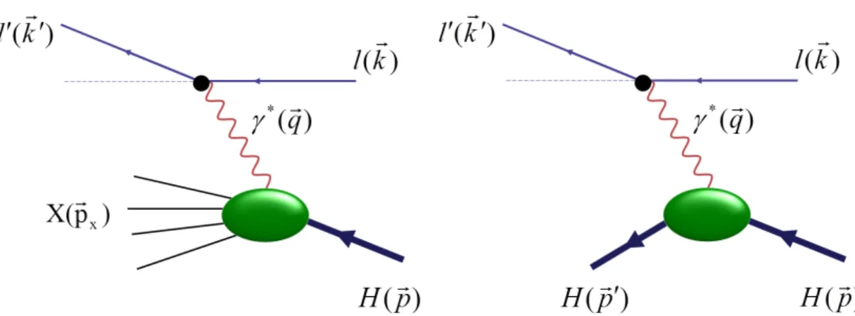
There exists different experiments for the study of hadron structure. These experiments are named with respect to their main focuses. When in a process an initial lepton with very short wavelength probes distances much shorter than the size of the target hadron, it is calleddeepprocess. When in a scattering process the incident and resultant particles are the same, like Compton scattering (right diagram of Fig.2.1.1), the process is called elastic scattering. While, when the target absorbs some energy and breaks up to many final particles, it is calledinelastic scattering (left diagram Fig. 2.1.1). So in deep inelastic scattering experiments, a high energy lepton interacts with the target hadron and breaks it to different other final states.

Moreover, if in a scattering process, more than a couple of final states are produced, different instruments are needed to detect the resultant particles. If only the scattered lepton is detected and the rest left unmeasured, it is called inclusive DIS. Whereas, when in addition to the scattered lepton, one or two high energy hadrons are detected, it is calledsemi-inclusive one. In the case that all final state particles and their momenta are known, it is called exclusive scattering. In the following, we discuss the exclusive DIS experiment and explain how these are used to obtain information about hadron structure functions therefrom.

1We follow [BR05] and [BP07], chapters 6 and 8 in [HM84], 2 and 3 in [Bas07], section 2 in [Sch98].

(16)

Figure 2.1.1: Left: Basic diagram for deep inelastic lepton-hadron scattering mediated by virtual photon exchange. Right: Elastic scattering, the hadron has exchanged its momentum, unlike the DIS process where hadron has been smashed into other particles.

2.1.1 Kinematics

DIS allows us to investigate the internal structure of hadrons. Most of our knowledge about hadron structures has been derived from lepton-hadron scattering

l(k) +H(p)→l⁰(k⁰) +X(px). (2.1.1) Here,l labels the initial lepton with 4-momentumk and energyE andl⁰ the outgoing lepton with 4-momentumk⁰ and scattered energyE⁰. X denotes all the final hadronic states with massMX. The kinematic variables describing the DIS process are

• Q² =−q²= (k−k⁰)² = 4EE⁰sin²(^θ₂): The squared 4-momentum transfer of the virtual photon.

• θ: Lepton scattering angle.

• ν = E−E⁰ = p·q/M_H: The energy loss of the lepton which can be associated with the energy of the virtual photonγ^∗.

• M_H: The mass of target hadron.

• p= (M, ~0): The 4-momentum of the fixed target.

• q= (E−E⁰, ~k−~k⁰): The 4-momentum of the virtual photon.

• y=ν/E: The fractional energy loss of the lepton.

• xB = _2M^Q²

Hν = _2p·q^Q² : The Bjorken scaling variable.

By increasingQ², the spatial resolution increases and the quark structure of the hadron can be seen.

(17)

2.1 Deep Inelastic Scattering (DIS) 2.1.2 Parton Model

DIS experiment is the key to evaluate parton densities,q(x), and Helicity distributions,

∆q(x), of hadrons [BP07]. A parton density is the probability of finding a parton with longitudinal momentum fraction x of its parent hadron, regardless of its spin directions. Helicity is the layout of a parton spin parallel or anti-parallel to the direction of the parent momentum. With respect to the positive helicity for parent, the number density of partons with positive helicity minus the negative ones is known as helicity distributions.

The basic idea of the parton model is that at high energy, an initial lepton interacts with one of the partons in the hadron by exchanging a virtual photon. It is shown schematically in Fig. 2.1.2. The structureless feature of partons is symbolized by the point notation in the Figure. To the lowest order, the interacting parton is a quark, since the gluon has no electric charge. All information about the target hadron in inclusive scattering processes are collected in the structure functions. We will see that to leading order at high energy momentum transferQ²→ ∞, the hadron structure functions are independent of the dimensional parameterQ² but depend on the fixed scaling variable xB proposed by Bjorken [BP69], which can be obtained from the invariant mass of the hadronic states

M_X² = (p+q)²=M²+ 2p·q+q². (2.1.2) Here, M_X at least must be the same as the mass of the hadron M_X² ≥ M². By implementingq²=−Q² in Eq. (2.1.2) we obtain

M²+ 2p·q−Q²≥M² ⇒ xB= Q²

2p·q ≤1. (2.1.3) It means that the longitudinal momentum fraction x is equal to the Bjorken scaling variablex_B. Since Q² and p·q are both positive, it follows that

0≤x_B ≤1 (2.1.4)

where x_B = 1 corresponds to elastic scattering (M_X² = M²). Also the lepton energy lossE−E⁰ is between zero (if E=E⁰) andE (ifE⁰ = 0), so the fractional energy loss of the lepton must be in the interval

0≤y≤1. (2.1.5)

2.1.3 DIS Cross Section

Studying the total cross section of a process is the first step towards an understanding the structure of hadrons [Jaf75]. The meaning of a cross section can be illustrated as follows; if an arrow is fired towards a ball, by increasing the radius of the ball the chance of hitting would go up and the cross section area will increase. However, in particle physics it is more complicated than in archery. In an experiment, the target is not a solid ball but a soft one. Moreover, because of different involved interactions,

(18)

Figure 2.1.2: Kinematics of lepton-hadron scattering in the parton model. The photon interacts with a single quark of the hadron.

the cross section depends on the nature of the fired arrow and the target both. Also, the incident particle can be scattered to different angles. The probability of interaction with particular scattered angle is measured by the differential cross section².

The differential cross section for the unpolarized DIS in the laboratory frame can be written as

dσ=X

X

Z d³k⁰

(2π)³2E⁰(2π)⁴δ⁴(k+p−k⁰−Xp) |M|²

2E2M. (2.1.6) Here, Mis the scattering amplitude containing all information about the interaction.

The polarization of the final lepton and hadrons have to be summed over. According to the factorization theorem, the spin-averaged M factorizes into the leptonic tensor also called hard part,Lµν, and the hadronic tensor called soft part,Wµν, as

|M|² ∼L^µνW_µν (2.1.7)

where Lµν and Wµν can be calculated perturbatively and non-perturbatively, respectively. The advantage of studying lepton-hadron scattering but not hadron-hadron scattering is that the lepton is a point-like particle. Therefore, the exact expression for Lµν can be written

L_µν = X final states

hk⁰|J_l^ν(0)|k, s_lihk, s_l|J_l^µ(0)|k⁰i (2.1.8) whereJ_l is the leptonic current.

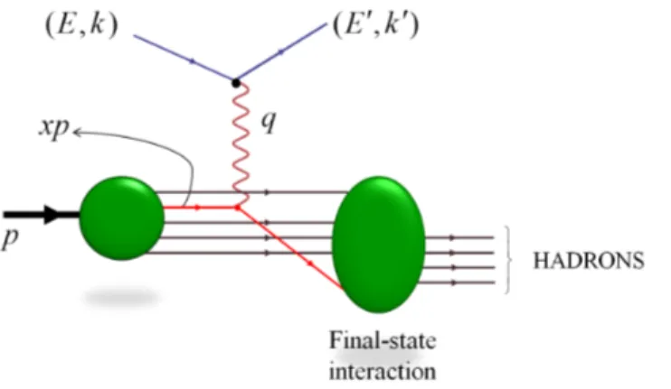
The hadronic tensor W^µν (shown in Fig.2.1.3) contains all information about the hadrons involved in the process. Its calculation is much more complicated. Hadronic tensor can be expressed as the imaginary part of the forward scattering amplitude in deeply virtual Compton scattering

W^µν = 1

2πImT^µν (2.1.9)

2We mostly follow [Gri08,Sch98,Man92] and references therein.

(19)

2.1 Deep Inelastic Scattering (DIS)

Figure 2.1.3: Hadronic tensor of deep inelastic scattering cross section. It detects the imaginary part of the forward Compton scatteringγ^∗(q)H(p)→γ^∗(q)H(p) [BR05].

where

T^µν =i Z

d⁴z e^iq·zhp, λ⁰|T {J^µ(z)J^ν(0)}|p, λi. (2.1.10) Here,T {J^µ(z)J^ν(0)}is the time-ordered product of the currentsJ^µ(z) andJ^ν(0). This relation is known as the optical theorem. So

W^µν =X

λ,λ⁰

1 4π

Z

d⁴z e^iq·zhp, λ⁰|J^µ(z), J^ν(0)|p, λi (2.1.11) whereλ(λ⁰) is the polarization of the initial (final) hadrons. Fig.2.1.4 illustrates this relation.

The hadronic tensorW^µν can be written in terms of a spin dependent part which is anti-symmetric and a spin independent one which is symmetric. The polarized lepton and polarized target produce the anti-symmetric leptonic tensor and anti-symmetric hadronic one. The product of these anti-symmetric leptonic and hadronic tensors results in the polarized form factors. In contrast, in unpolarized scattering, one averages over the target polarization and the spin dependent part ofW^µν vanishes. Therefore, using an unpolarized lepton beam and an unpolarized hadron target is sufficient to measure unpolarized form factors [Bas07].

The spin independent part ofW^µν decompose into two unpolarized structure functions,F₁ and F₂, which depend on two Lorentz invariant quantities

W^µν =−F₁(xB, Q²)

g^µν−q^µq^ν q²

+ F2(xB, Q²) p·q

p^µ−p.q q² q^µ

p^ν− p.q q² q^ν

. (2.1.12) Here,Q²=−(p_l−p_l⁰)² <0 is the squared four-momentum transfer by virtual photon.

It is known as the scale (resolution) to probe the inner structure of the hadron.

In the Bjorken limit, Q² → ∞, structure functions depend only on x_B. These Bjorken scaling functions are related to each other by the Callan-Gross relation [CG69]

F1(x) = 1

2xF2(x) (2.1.13)

with

F₂(x) =X

q

e²_qx q_q(x) (2.1.14)

(20)

Figure 2.1.4: The optical theorem: the total cross section of the DIS is equal to the imaginary part of the forward Compton scattering. Inspiration for this figure is from [G⁺13].

where eq denotes the electric charge of the struck parton. q(xB) is the probability of finding a parton q with a longitudinal momentum x

q(x) = (q↑+q↓)(x) + (¯q↑+ ¯q↓)(x) (2.1.15) which is called parton distribution function (PDF). Eq. (2.1.13) is a result of the fact that fermions which are involved partons in DIS are spin 1/2 particles [Pic95].

2.2 Deeply Virtual Compton Scattering

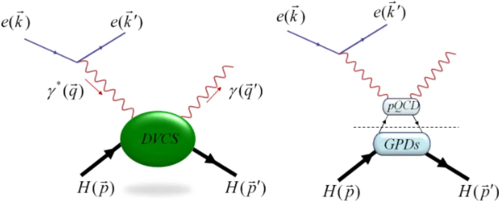
A modern framework to describe the parton structure in hadrons is given by so-called Generalized Parton Distribution functions (GPDs). Experimentally, GPDs can be measured viaVirtual Compton Scatteringwhich means at least one of the photons involved in the Compton scattering is virtual. VCS amplitude is similar to the hadronic tensor of DIS (see Fig.2.1.3). Since in the Bjorken limit the momentum transfer is large, in this region virtual Compton scattering is also known as deeply virtual Compton scattering which was proposed by Ji [Ji97] and Radyushkin [Rad96]. DVCS is a hard exclusive process in which the lepton interacts with the hadron via a virtual photon under the emission of another photon. The reaction is represented as

l(k) +H(p)→l⁰(k⁰) +H(p⁰) +γ(q⁰). (2.2.1) DVCS, schematically is illustrated in Fig.2.2.1.

2.2.1 Definition and Properties of GPDs

A current can be constructed from combinations of Γ matrices and Dirac fields, ¯ψΓψ.

Matrix elements of those currents can be expressed in terms of form factors with covariant normalization hp⁰|pi = 2p⁰(2π)³δ(p⁰ −p), where (p^µ) and (p^0µ) are the initial and final momentum, respectively³.

DIS and DVCS have similar kinematics. DIS involves forward matrix elements of certain operators (p^µ = p^0µ) which encode the information about parton distribution

3For this section we follow [Rad96,Rad97,Die03,BR05,Cou10]

(21)

2.2 Deeply Virtual Compton Scattering

Figure 2.2.1: Left: schematic diagram of DVCS scattering. At least one of two involved photons is virtual. Right: the leading-order handbag diagram. DVCS factorizes into hard parts which is calculable by perturbation theory (pQCD) and the soft parts (GPDs) which can be measured non-perturbatively.

functions (PDFs). DVCS experiments on the other hand include off-forward matrix elements (p^µ6=p^0µ) and these matrix elements can be parametrized in terms of generalized parton distributions (GPDs).

PDFs are Q²-independent but depend on momentum fraction x. However, GPDs are off-forward, so they are functions ofQ²

Q² =−t=−∆² =−(p⁰−p)². (2.2.2) Moreover, GPDs require additional variables to describe the initial and final parton states. It is the so-called skewnessξ, which is the longitudinal momentum asymmetry

ξ=−n·∆

2P ·n = p⁺−p⁰⁺

p⁺+p⁰⁺. (2.2.3)

Here,nis the light-like four-vector,n±= (1,0,0,±1)/√

2 andp⁺andp⁰⁺are used for the pion momenta in light-cone coordinates which is defined byv^±= ^√¹

2(v⁰±v³) =vn∓4. Schematics of DIS, DVCS and elastic scattering are illustrated in Fig.2.2.2. Regarding ξ, one can split momentum fractionx into the three different regions [Die03]:

• x∈ [−1,−ξ], both partons have negative momenta −(x−ξ) and −(x+ξ), and this corresponds to the emission and absorption of anti-quarks.

• −ξ < x < ξ, one parton has positive momentum while the other one has negative.

It corresponds to the emission of a quark and an anti-quark. In this area GPDs behave like meson distribution amplitudes of finding quark and anti-quark pair.

However, this kind of information is relatively unknown and can not be accessed in DIS.

• x∈[ξ,1], both partons have positive momenta (x−ξ) and (x+ξ), which corresponds to the emission of a quark and then absorption of a quark.

4For the comprehensive explanation look at [Col97].

(22)

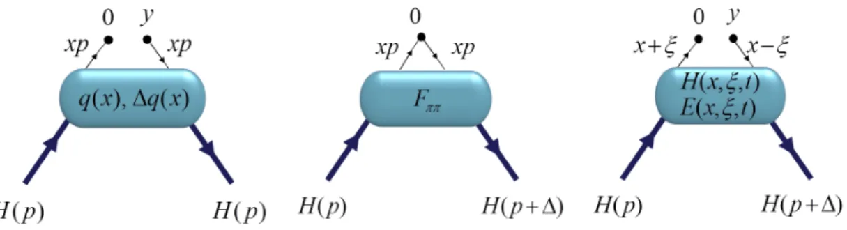
Figure 2.2.2: Left: non-local forward matrix elements hp|ψ¯q(0)Γψq(y)|pi accessed in DIS. Middle: local off-forward matrix elements hp⁰|ψ¯_q(0)Γψ_q(0)|pi accessed in elastic lepton-hadron scattering. Right: non-local off-forward matrix element hp⁰|ψ¯q(0)Γψq(y)|pi accessed in DVCS in the region −ξ < x < ξ.

Similarly to DIS experiment, the cross section of a DVCS process can be factorized into a hard part which can be calculated perturbatively and a soft part which is a non- perturbative quantity [JO98]. This decomposition is often called a handbag diagram illustrated in Fig. 2.2.1.

GPDs, representing the soft part of the scattering, are defined through a Fourier transform of matrix elements of quark and gluon operators at a light-like separation.

The gluon operators will not be considered in our work. The bilocal quark operators are defined as [Hag10]

O^q_Γ(x) = Z +∞

−∞

dz

2πe^ixz·nq(−z

2 ·n) ΓW_[−^z

2·n,^z₂·n]q(z

2·n) (2.2.4) wherexis the momentum fraction of the quark and Γ has the Dirac structures Γ =γ^µ, γ^µγ⁵,iσ^µν to construct the axial, vector and tensor operators. W is a Wilson line along a light-like path between two quarks to guaranty the gauge invariance of the matrix elements

W =Pexp

ig Z −^z

2

z 2

dx n·A(xn)

. (2.2.5)

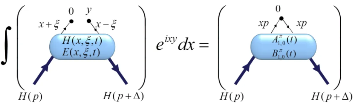
Here,P represent a path ordered integral andn·Aindicates the light-cone gauge. The pion GPDs for vector and tensor operators are then described by [Die03]

hπ(~p⁰)|O^µ_V(x)|π(~p)i= 2¯p^µH^π(x, ξ, t) + higher twist, (2.2.6) hπ(~p⁰)|O^µν_T (x)|π(~p)i= p¯^[µ∆^ν]

mπ

E_T^π(x, ξ, t) + higher twist (2.2.7) with definition ofA^[µB^ν] =A^µB^ν −A^νB^µ. H^π(x, ξ, t) and E_T^π(x, ξ, t) are unpolarized form factors since it is averaged over the quark helicities.

Forward Limit

The matrix elements in Eq. (2.2.6) and (2.2.7) are off-forward because the momenta of the initial and final hadrons are different. In the forward limit, p = p⁰, hence

(23)

2.3 Moments of GPDs

∆ =p−p⁰ = 0 andξ= 0. It means the fraction of the longitudinal momentum carried by the struck parton is the Bjorken variable x → x_B. As a result, the generalized parton distributions in the forward limit are reduced to ordinary parton distributions calculated in DIS [BP07]

H^π(xB,0,0) =

q(x_B), x_B>0

−¯q(−x_B), xB<0. (2.2.8) Parton distribution functions (PDFs) are the probability to find a parton with momentum fraction 0≤x≤1.

2.3 Moments of GPDs

Eq. (2.1.10) indicated that by means of the optical theorem, deep inelastic structure functions can be determined by the commutator of two non-local currentsJ^µ(z)J^ν(0), sandwiched between hadronic states. At short distances, around the light-conez² →0, the currents product can be expanded into a series of local operators [WZ72]

lim

z²→0O_i(z)O_j(0) =X

k

cijk(z)O_k(0) (2.3.1) wherecijk called Wilson coefficients which depend on the separation z. This is called an operator product expansion (OPE). Hence, to compute the matrix elements, the operator product can be replaced by the expansion (2.3.1) where the Wilson coefficients are independent of the matrix elements [GW73a]. The same OPE holds for virtual Compton structure functions as well [MV00].

The matrix elements of operators in the hadronic tensor correspond to the Mellin moments of the structure function. The Mellinn–th moment of a functionf is defined as [C⁺72]

M_n= Z ₁

0

dx xⁿ⁻¹f(x), n= 1,2, . . . . (2.3.2) The inverse of all Mellin moments would give us the function f.

Twist-two Operators

By means of the OPE, instead of the light-cone operators, tower of local operators O^µ_n¹^···µⁿ which are traceless and symmetric inµ_iare used. In DIS kinematics, 0< x_B=

Q²

2MHν <1 and an operator with dimensiondand spinnis of orderO(x⁻ⁿ_B )(M_H/Q²)^d−n−2. It means an operator being controlled by exponent ofd−n−2, whered−nis [GT71]

twist = dimension (d)−spin (n). (2.3.3) The minimal twist (= 2) has the main contributions which corresponds to maximal spin. A finite amount of twist-two operators are contributing to the structure functions in the deep inelastic limit. The twist-two operators are written in terms of quark fields ψ, gluon fieldsF_µν and covariant derivativesD^µ. Their spin, dimension and twists are

(24)

ψ F_µν D^µ

d ³₂ 2 1

n ¹₂ 1 1

t 1 1 0

Table 2.3.1: Dimension and twist.

listed in Table2.3.1. Note that adding derivatives to the operator will not change the twist, because spin and dimension both increase by one and according to Eq. (2.3.3), their contributions in changing twist is zero. The twist-two operators for quark and gluon have different forms. The gluonic operators are not discussed here and the general forms of traceless twist-two operators for quarks are written as (see, e.g., [Sch98])

O_{M q}^{µ¹^···µⁿ^} =iⁿ⁻¹ψ¯^(f⁾γ^{µ¹←→

D^µ²· · ·←→

D^µⁿ^}ψ^(f⁰⁾, (2.3.4) O_{M σq}^[µ¹^{ν]···µⁿ^} =iⁿ⁻¹ψ¯^(f⁾iσ^[µ¹^{ν]←→

D^µ²· · ·←→

D^µⁿ^}ψ^(f⁰⁾ (2.3.5) whereψ^(f) denotes a quark field with flavorf,←→

Dµ= ¹₂(−→ Dµ−←−

Dµ) is the symmetrized covariant derivative,σ_µν =i/2[γ_µ, γ_ν]. The notation{µ₁µ₂}indicates the symmetrization inµ₁ andµ₂ and [µ₁ν] anti-symmetrization inµ₁ andν. We should note that one at first has to symmetrize and then anti-symmetrize the indices, i.e. for example

O^[µ¹^{ν]µ²^} =1

2(O^{µ¹^ν}µ² +O^{µ¹^µ²^}ν)

=1

4(O^µ¹^νµ²− O^νµ¹^µ²+O^µ¹^µ²^ν− O^µ²^µ¹^ν). (2.3.6)

2.4 Generalized Form Factors

The off-forward pion matrix elements of a local vector operator for the first moment (n= 1) reads

hπ(~p⁰)|ψ¯_q(0)γ^µψ_q(0)|π(~p)i= 2¯p^µA^π_1,0(t). (2.4.1) Here,A^π_1,0(t) corresponds to the single pion form factorfππ(t), which counts the number of valence quarks of one flavor inside the pion. Similarly, the off-forward pion matrix element of a local tensor operator forn= 1 is parametrized by

hπ(~p⁰)|ψ¯q(0)iσ^µνψq(0)|π(~p)i= p¯^[µ∆^ν]

mπ

B^π_T_1,0(t) (2.4.2) whereB_T^π_1,0 denotes the pion tensor form factors. BothA^π_1,0(t) and B_T^π_1,0(t) are functions of momentum transfertand independent ofξ[Die03]. Comparing Eq. (2.4.1) and (2.4.2) with (2.2.6) and (2.2.7) respectively gives the following sum rules [Ji97]

Z +1

−1

dx H^π(x, ξ, t) =A^π_1,0(t), (2.4.3) Z ₊₁

−1

dx E_T^π(x, ξ, t) =B_T^π_1,0(t). (2.4.4)

(25)

2.4 Generalized Form Factors

Figure 2.4.1: Sum rules to link the first moment of the GPDs to their GFFs.

Here, the negative x region −1 < x < 0 corresponds to an anti-quark distributions.

These sum rules are illustrated in Fig. 2.4.1. In order to get the full form factor, we have to sum over all flavors.

The second moment (n= 2) of the off-forward pion matrix elements of twist-two vector and tensor operators can be parametrized by generalized form factors (GFFs)

hπ(~p⁰)|O_V^µν(0)|π(~p)i= 2¯p^µp¯^νA^π_2,0(t) + 2∆^µ∆^νC_2,0^π (t), (2.4.5) hπ(~p⁰)|O^µνρ_T (0)|π(~p)i=A_µνS_νρp¯^µ∆^ν

mπ

¯

p^ρB_T^π_2,0(t) (2.4.6) where A^π_2,0, C_2,0^π and B_T^π_2,0 represent the pion generalized form factors and A and S are functions to anti-smmetrize and symmetrize the indices which were explained in Eq. (2.3.6). The second moments of the pion GPDs are equivalent to GFFs by using Mellin transformation

Z +1

−1

dx x H^π(x, ξ, t) =A^π_2,0(t) + (−2ξ)²C_2,0^π (t), (2.4.7) Z +1

−1

dx x E_T^π(x, ξ, t) =B_T^π_2,0(t). (2.4.8) In the forward limit (∆→0, ξ →0), A^π_2,0(0) simplifies to

hxi^π = Z 1

−1

dx x q^π(x) =A^π_2,0(t= 0) (2.4.9) which is interpreted as the momentum fraction carried by partons in the pion.

Now we can write the general form of the matrix elements of the tower of twist-two operators between unequal momentum states. All possible form factors for the vector quark operators arise [Ji98]

hπ(~p⁰)|O^{µ_q ¹^···µⁿ^}|π(p)i= (2.4.10) 2¯p^{µ¹p¯^µ²· · ·p¯^µⁿ^}An,0(t) + 2

n

X

i=0 odd

∆^{µ¹∆^µ²· · ·∆^µⁱP^µⁱ⁺¹· · ·P^µⁿ^}Cn,i(t)

(26)

and for tensor operators

hπ(~p⁰)|O^[µ_σq¹^{ν]µ²^···µⁿ^}|π(p)i= 1 m_π

n

X

eveni=0

¯

p^[µ¹∆^{ν]∆^µ²· · ·∆^µⁱp¯^µⁱ⁺¹· · ·p¯^µⁿ^}B_{T n,i}(t).

(2.4.11) Note that for the tensor operator, one has to first symmetrize and then anti-symmetrize [G⁺99a]. The higher moments of GPDs for twist-two operators are related with GFFs as

Z +1

−1

dx xⁿ⁻¹H^π(x, ξ, t) =A^π_n,0(t) +

n

X

i=1odd

(−2ξ)ⁱ⁺¹C_n,i+1^π (t), (2.4.12) Z +1

−1

dx xⁿ⁻¹E^π(x, ξ, t) =B_{T n,0}^π (t). (2.4.13) In case that ξ= 0, the information from PDFs and form factors are combined and GPD(x,0, t) can be explained as the probability of finding a quark with longitudinal momentum fractionx at a given transverse distance in the hadron [G⁺13].

2.5 Pion Electromagnetic Form factor

In elastic processes, soft physics at the long distance are parametrized in terms of form factors. A form factor is a function that gives the information about a certain particles interaction. It is measured experimentally by

dσ

dΩ = dσ dΩ

point-like |f_ππ(q²)|² (2.5.1) wheredΩ is the solid angle and f_ππ(q²) denotes the form factor at momentum transfer q =k⁰ −k. Since the pion is a spinless particle, the Lorentz decomposition of matrix elements for current Jem^µ provides only one electromagnetic form factor (Eq. (2.4.1))

hπ(~p⁰)|J_em^µ (~p⁰−~p)|π(~p)i= 2¯p^µf_ππ(t) with t≡∆² = (p⁰−p)² (2.5.2) where p and p⁰ are the incoming and outgoing momenta, t is the momentum transfer and ¯p^µ = (p⁰+p)/2. The form factor f_ππ describes the charge distribution of a pion, that is the deviation of a pion from being a point-like charge interacting with the electromagnetic field. There have been early measurements of the pion form factors (see, e.g., [B⁺78,A⁺86,B⁺83,H⁺08b,H⁺06]).

2.5.1 The pion Charge Radius

We are interested in the cross section for scattering leptons from a point charge to deduce the structure of the target from the form factor. The form factor for a static target can be written as the Fourier transform of the charge distribution [Hof56]

f_ππ(q²) = Z

ρ(r⁰)e^−iq·r⁰d³r⁰ (2.5.3)

(27)

2.5 Pion Electromagnetic Form factor

Figure 2.5.1: Spherical coordinates to describe the volume element.

where d³r⁰is the volume element andρ(r⁰) is the charge distribution which is normalized as

Z

ρ(r⁰) d³r⁰ =1 (2.5.4)

whereρ is assumed to be spherically symmetric. Spherical coordinates can be chosen to describe the volume element as shown in Fig. 2.5.1when q is parallel to z-axis. So, the volume element is driven as d³r⁰ = r⁰²dr⁰d(cosθ) dφ. By integrating Eq. (2.5.3) utilized Eq. (2.5.4) one finds

fππ(q²) =

Z Z Z

r⁰²dr⁰d(cosθ) dφ ρ(r⁰)e^−iqr⁰^cos^θ (2.5.5)

= Z _2π

0

dφ Z

r⁰

Z ₁

−1

r⁰²dr⁰d(cosθ)ρ(r⁰)e^−iqr⁰^cos^θ (2.5.6)

= Z

r⁰

2π[ 1

iqr⁰e^−iqr⁰^cos^θ]¹₋₁ρ(r⁰) r⁰²dr⁰. (2.5.7) With the definition of the sine function with complex arguments we obtain

f_ππ(q²) = Z

r⁰

4πsin(qr⁰)

qr⁰ ρ(r⁰) r⁰²dr⁰. (2.5.8) If the momentum transfer|q|is not too large, we can Taylor expand sinx =x−^x_3!³ +

x⁵

5! +· · · and with Eq. (2.5.4) obtain

fππ(q²) = 1 +1

6q²hr²i+· · · (2.5.9) where hr²i ≡ R

r⁰²ρ(r⁰) d³r⁰ ≡ 6|^df_dq^(q₂²⁾|_q2=0 known as a charge radius. By using the normalization condition Eq. (2.5.4), we obtain

fππ(0)≡1. (2.5.10)

In the limit |q| → 0, the exchanged photon has the energy much smaller than the energies of the participating particles in a particular scattering process. However, the wavelength is large enough to resolve only the size of the charge distributionρ but it is not sensitive to its detailed structures.

(28)

(29)

Chapter 3

Quantum Chromodynamics on the Lattice

Quantum chromodynamics (QCD) is the theory of the strong force describing the interactions between quarks and gluons. QCD is a quantum field theory with a non-abelian gauge symmetry, given by the groupSU(3).

Strong interactions phenomena cover a large range of energies. Their descriptions within the framework of QCD however, requires different techniques. Perturbation theory is perfectly fitted for the high energy range where QCD behaves asymptotically free. At low and intermediate scales, perturbative QCD is not applicable anymore, but there is lattice QCD which enables us to treat many strong interactions phenomena non-perturbatively.

Before giving a brief summary of lattice QCD, we will look at the continuum formulation which will assist us to map the theory onto a four dimensional lattice grid.

In continuum calculations, Minkowski space-time is utilized where a space-time point is given by a 4-vector, sayx^µ. It is a combination of the three ordinary dimensions of space withµ= 1,2,3 for three space directions and a single dimension of time, µ= 0.

The explanation of this chapter mainly follows the text books [PS95,Gri08,GL10].

3.1 QCD in the Continuum

The QCD action is defined by the space-time integral over the QCD Lagrange density L_QCD

S_QCD = Z

d⁴x L_QCD =S_{f erm}+S_gluon. (3.1.1) It consists of a fermionic¹ part, S_{f erm} which describes the dynamics of quarks (anti- quarks) and their interactions with the gauge fields and a gluonic² part, S_gluon which encodes the dynamics of the gauge fields and their self interactions.

1A fermion is a half-integral spin particle and obeying the Pauli exclusion principle.

2In particle physics, gluons (or gauge bosons) are the exchange particles for the strong force between quarks.

(30)

Quark and anti-quarks are fermions which are represented by a Dirac 4-spinors ψ_α,a^f (x),ψ¯_α,a^f (x) (3.1.2) at a given space-time position. Here, α∈[1,2,3,4] stands for Dirac index,a∈[1,2,3]

color index, i.e. green, red, blue and f ∈[1, . . . , N_f] flavor index. Hence every quark flavorψ^f(x) comes with 12 independent components.

3.1.1 The Fermion Action

The dynamics of the quarks and gluons is given by the Quantum Chromodynamics Lagrangian. In Euclidean space, the Dirac Lagrangian for a non-interacting quark with flavorf and massm^f is written as³

L_Dirac= ¯ψ^f(x)(γµ∂µ+m^f)ψ^f(x) (3.1.3) where the Euclidean Dirac matricesγ_µ withµ= 1,2,3,4 are defined in AppendixA.3.

We want to haveL_Dirac invariant under a symmetry transformation at some space- time points called local gauge transformation as

ψ(x)→ψ⁰(x) = Λ(x)ψ(x),

ψ(x)¯ →ψ¯⁰(x) = ¯ψ(x)Λ⁻¹(x) (3.1.4) where Λ∈Ris defined as

Λ(x) =eîθ(x) =eîωâ^(x)Tâ. (3.1.5) Here, ωâ(x) ∈ R parametrize the group and they are space-dependent. Tâ are generators of the SU(N) group (in QCD, N = 3, they calledGell-Mann matrices which are traceless and Hermitian⁴ [Geo99]). The normalization of the generators is fixed by imposing tr(TâT^b) =δâb/2. The property of tr(Tâ) = 0 andTâ =T^†a satisfy the commutator relationship

[T^a, T^b] =i

N²−1

X

c=1

f^abcT^c (3.1.6)

wheref^abc are real numbers calledanti-symmetric structure constants.

But the above Lagrangian, Eq. (3.1.3), is not invariant under this local gauge transformation since we pick up an extra term from the derivative of theθ(x) in Eq. (3.1.5).

To guarantee the local gauge invariance of the Lagrangian, every usual derivative is replaced by the covariant derivativeD_µ(x) as

D_µ(x) =∂_µ+iA_µ(x), with ∂_µ=∂/∂x^µ, A_µ(x) =

8

X

a=1

Aâ_µ(x)Tâ, Aâ_µ(x)∈R. (3.1.7)

3The Dirac Lagrangian in Minkowski space isLDirac= ¯ψ^f(x)(iγ^µ∂µ−m^f)ψ.

4Hermitian operator is an operator coincident with its adjoint.

(31)

3.1 QCD in the Continuum

A_µ(x) is the four-vector potential. It is necessary to know the transformation for the gauge field in order to preserve the gauge invariance

L[ψ(x),ψ(x), A¯ _µ(x)] =L[ψ⁰(x),ψ¯⁰(x), A⁰_µ(x)]. (3.1.8) By inserting Eq. (3.1.4) on the right hand side of Eq. (3.1.8) we obtain

L[ψ(x),ψ(x), A¯ µ(x)]= ¯^! ψ(x)Λ⁻¹(x) γµ(∂µ+iA⁰_µ(x)) +m

Λ(x)ψ(x). (3.1.9) The mass term cancels out and the rest is

ψ(x)¯ ∂_µ+iA_µ(x)

ψ(x)=^! (3.1.10)

ψ(x)Λ¯ ⁻¹(x) ∂µ+iA⁰_µ(x)

Λ(x)ψ(x).

Using the product rule for∂µ in the right hand side produces an additional term ψ(x)¯ ∂µ+iAµ(x)

ψ(x)= ¯^!ψ(x)∂µψ(x) + ¯ψ(x)Λ⁻¹(x)(∂µΛ(x))ψ(x) (3.1.11) +iψ(x)Λ¯ ⁻¹(x)A⁰_µ(x)Λ(x)ψ(x).

It should be denoted that Λ(x) commutes with theγ_µ matrices since γ_µ acts in Dirac space but Λ(x) acts in color space. Considering Λ^†(x) = Λ⁻¹(x) and solving forA⁰_µ(x) gives us the transformation law for the gauge fields

Aµ→A⁰_µ(x) = Λ(x)Aµ(x)Λ⁻¹(x) +i(∂µΛ(x))Λ⁻¹(x). (3.1.12) Now we can write the fermionic part of QCD

S_{f erm}[ψ,ψ, A] =¯

nf

X

f=1

Z

d⁴xψ¯^f(x)(γ_µD_µ+m^f)ψ^f(x). (3.1.13)

3.1.2 The Gauge Field Action

In QCD, gluons mediate the strong interactions of quarks, and they carry color/anti- color charges. They are massless particles, so their Lagrangian contains only the mass term. The field strength tensorFµν(x) is defined as the commutator of the covariant derivatives

Fµν(x) =−i[D_µ(x), Dν(x)] =∂µAν(x)−∂νAµ(x) +i[Aµ(x), Aν(x)]

=

8

X

a=1

h

∂µAâ_ν(x)−∂νAâ_µ(x)−fâbcA^b_µ(x)A^c_ν(x) i

T^a

=

8

X

a=1

F_µν^a (x)T^a. (3.1.14)

Note that in QCD, the commutator [Aµ(x), Aν(x)] does not vanish and in the second line relation (3.1.6) was used. If the field has a local transformation law, its covariant

(32)

derivative holds the same law and the commutator of the covariant derivatives as well.

Therefore, it is clear thatF_µν(x) under the Eq. (3.1.12) transforms as

F_µν(x)→F_µν⁰ (x) = Λ(x)F_µνΛ⁻¹(x). (3.1.15) Two field strength tensors contract to maintain Lorentz symmetry and take the trace to preserve the gauge symmetry. The gauge action then is given by

S_G(x) =− 1 2g²

Z

d⁴x tr[F_µν(x)F_µν(x)] =− 1 4g²

8

X

a=1

F_µν^a (x)F_µν^a (x). (3.1.16)

3.2 QCD on the Lattice

Lattice gauge theory was introduced by K. Wilson in 1974 [Wil74]. On a hypercubic grid with spacing a = a_s = a_T, quark fields are placed on sites and gauge fields on the links between sites. So fermion and gluon fields, derivatives, integrals and so on have to be replaced by discretized expressions. For the lattice QCD, we switch from Minkowski to Euclidean space. This allows us to estimate path integrals by means of Monte Carlo integrations. These simulations are used to calculate correlation functions on the lattice. AD-dimensional Minkowski field theory (D−1 spatial dimensions and one time dimension) is connected to a D-dimensional Euclidean field theory by using Wick rotation

x⁰_M ≡t→ −ix₄≡ −iτ, x^j_M ≡x^E_j (3.2.1)

p⁰_M ≡E →ip₄, p^j_M ≡p^E_j . (3.2.2)

There are different ways in which the QCD action can be discretized and all must give consistent results in the continuum limit. The purpose of this introduction is to provide an outline about the results that are presented in other sections for correlation functions, effective masses and calculation of matrix elements. For a comprehensive explanation of lattice QCD we found the following books [GL10,TC06, L⁺11, Fle88]

and reviews of [Gup97,Het12,Gut12] really helpful.

3.2.1 Discretization and Formulation of Lattice Action

First of all we have to introduce the number of nodes in 4-dimensional space-time

x=a





 x1

x₂ x₃ x4







with x₁, x₂, x₃∈ {0,1,· · · , N_L−1}, (3.2.3)