https://doi.org/10.1140/epjc/s10052-018-5700-9 Regular Article - Theoretical Physics
Pion distribution amplitude from Euclidean correlation functions
Gunnar S. Bali1,2, Vladimir M. Braun1, Benjamin Gläßle1, Meinulf Göckeler1, Michael Gruber1, Fabian Hutzler1, Piotr Korcyl1,3, Bernhard Lang1, Andreas Schäfer1, Philipp Wein1,a, Jian-Hui Zhang1
1Institut für Theoretische Physik, Universität Regensburg, Universitätsstraße 31, 93040 Regensburg, Germany
2Department of Theoretical Physics, Tata Institute of Fundamental Research, Homi Bhabha Road, Mumbai 400005, India
3Marian Smoluchowski Institute of Physics, Jagiellonian University, ul. Łojasiewicza 11, 30-348 Kraków, Poland
Received: 22 December 2017 / Accepted: 4 March 2018
© The Author(s) 2018
Abstract Following the proposal in (Braun and Müller. Eur Phys J C55:349,2008), we study the feasibility to calculate the pion distribution amplitude (DA) from suitably chosen Euclidean correlation functions at large momentum. In our lattice study we employ the novel momentum smearing tech- nique (Bali et al. Phys Rev D93:094515,2016; Bali et al.
Phys Lett B774:91,2017). This approach is complementary to the calculations of the lowest moments of the DA using the Wilson operator product expansion and avoids mixing with lower dimensional local operators on the lattice. The theoretical status of this method is similar to that of quasi- distributions (Ji. Phys Rev Lett 110:262002,2013) that have recently been used in (Zhang et al. Phys Rev D95:094514, 2017) to estimate the twist two pion DA. The similarities and differences between these two techniques are highlighted.
1 Introduction
In recent years there has been increasing interest in the possibility to determine parton distribution functions from Euclidean correlation functions, bypassing Wilson’s opera- tor product expansion. The general scheme of such calcula- tions is to consider a product of suitable local currents at a spacelike separationz, sandwiched between hadronic states, H|
¯ qΓ1Q
(z/2)QΓ¯ 2q
(−z/2)|H, (1)
and match the lattice calculation of this quantity to the per- turbative expansion in terms of collinear parton distributions H| ¯q(n)Γq(−n)|H, n2=0. (2) The existing concrete proposals differ mainly in the choice of theQ-field. This can be chosen as an auxiliary scalar in
ae-mail:philipp.wein@physik.uni-r.de
the fundamental representation of the color group [6,7], or as an (auxiliary) heavy [8] or light [1] quark. Another sugges- tion [4] is to replace theQ-field propagator by a Wilson line connectingq¯(z/2)andq(−z/2). This last proposal received the most attention, despite added complications due to the renormalization of the Wilson line [9,10], see Refs. [11–18]
for recent discussions, the reason being that it allows for a more direct momentum space interpretation in the framework of the large-momentum effective theory [14,19] (LaMET).
The corresponding correlation functions, transformed into the longitudinal momentum fraction representation, have become known as quasi-parton-distributions [4]. While quasi parton-distributions are certainly interesting objects, it was already pointed out in Refs. [1,20] that position space correla- tion functions (or “lattice cross sections”, in the terminology of [21–23]) contain the complete information on parton dis- tributions. In all cases the functions calculated on the lattice (for early work, see also [24]) are related to parton distri- butions by means of QCD factorization in the continuum, which can be done both in position and momentum space.
A position space analysis naturally leads to the concept of Ioffe-time distributions [16,20,25,26]. We emphasize that all the above suggestions are equivalent, and their relative virtue will be determined by the possibility to control lattice artifacts and other systematic uncertainties.
In this work we study the simplest function of this kind, the pion distribution amplitude (DA), using the technique suggested in Ref. [1], i.e., we use a light quark (Q =q) in Eq. (1) and perform the analysis directly in position space.
The same DA has recently been studied using the quasi- distribution approach in Ref. [5]. We consider a correlation function of renormalized scalar and pseudoscalar operators at equal times
T(p·z,z2)= π0(p)|
¯ u q
(z/2)
¯ qγ5u
(−z/2)|0, (3)
whereq¯(z)creates a light quark field of hypothetical flavor q = u,d and square brackets [O] denote operator renor- malization in the MS scheme. In what follows, we fix the renormalization scale to the “kinematic” scale in the correla- tor,μR=2/√
−z2(cf. [1,27]). The correlation function (3) can be calculated on the lattice as a function of two variables, p·z= −p·zandz2= −z2. Here and below we use boldface letters for spatial 3-vectors.
We restrict ourselves to sufficiently small distances,
|z|/2 < 1 GeV−1, such that the same correlation function can be calculated in continuum perturbation theory in terms of the pion DA using standard QCD factorization techniques.
The result reads
T(p·z,z2)=Fπ p·z
2π2z4ΦπSP(p·z,z2) , (4) whereΦπSP=Φπ+O(αs)+ higher twist (the various cor- rections will be discussed later), with
Φπ(p·z)= 1
0
du ei(u−1/2)(p·z)φπ(u) . (5) Fπ ≈ 93 MeV is the pion decay constant, the variableu corresponds to the quark momentum fraction andφπ(u)is the (leading-twist) pion DA. The integral of the pion DA is normalized to unity,1
0duφπ(u) =1,and its shape has been hotly debated for more than 30 years. This discussion has been reinvigorated by the strong scaling violation in the πγ∗γ form factor observed by the BABAR [28] and, to a lesser extent, the BELLE [29] collaboration, which is difficult to explain unless the pion DA exhibits strong enhancements near the end points, see, e.g., Refs. [30–32] for a review and further references. For illustrative purposes we consider three models:
φπ(1)(u)=6u(1−u) ,
0.0 0.2 0.4 0.6 0.8 1.0
u
0.0 0.2 0.4 0.6 0.8 1.0 1.2 1.4 1.6
φ(i) π(u)
φ(1)π
φ(2)π
φ(3)π
Fig. 1 Plot of the three models for the pion distribution amplitude given in Eq. (6)
0 2 4 6 8 10
p·z
–0.2 0.0 0.2 0.4 0.6 0.8 1.0
Φπ(p·z)
φ(1)π
φ(2)π
φ(3)π
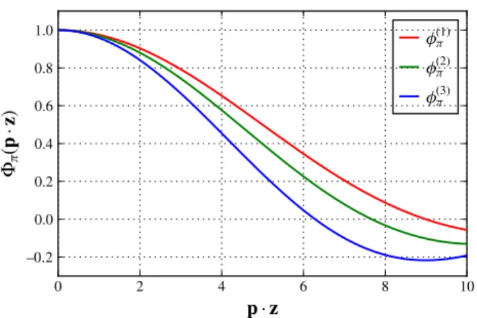
Fig. 2 The position space pion DAΦπ(p·z)[cf. Eq. (5)] for the three models in Eq. (6)
φπ(2)(u)= 8 π
u(1−u) ,
φπ(3)(u)=1, (6)
at the reference scale μ0 = 1 GeV. These models and the corresponding Fourier-transformed position space DAs Φπ(p·z), defined in Eq. (5), are plotted in Figs.1 and2, respectively. Measuring the correlation function (3) on the lattice for a range of values of p·z= −p·zandz2= −z2 gives access to the pion DA in position space (5) that contains the full information on the longitudinal momentum fraction distribution.
The main difference of our technique [1] to the approach of Ref. [5] is that the smallness of higher twist and perturba- tive corrections (forarbitrarypion momentum) is guaranteed by keeping the distance|z|between the currents sufficiently small. A large pion momentum is needed not in order to sup- press the corrections, but because it provides the necessary lever arm in the dimensionless variablep·zthat is manda- tory to distinguish between pion DAs of different shape, see Fig.2.
In contrast, in the LaMET-based approach of [5] formally a Fourier transform over all values ofzis taken, and small- ness of perturbative and higher twist corrections is achieved indirectly by considering the asymptotic expansion of the amplitude at large values of the pion momentum for a fixed quark momentum fractionu, which is the Fourier conjugate ofp·z. Thus|p| → ∞implies that the integration region in the Fourier integral shrinks to|z| ∼1/|p| →0.
Another difference is that in Ref. [5] a Wilson line is used to connect the quark and the antiquark, whereas in this study we use a light-quark propagator [1]. To tree-level accuracy the difference in the corresponding coordinate space expres- sions is simply a different coefficient function in Eq. (4).
While taking the Wilson line not along a lattice axis intro- duces additional difficulties, e.g., concerning renormaliza- tion, the separationzcan be chosen arbitrarily without prob-
lems when a light-quark propagator is used. We consider this possibility as an advantage of our calculation because we have found discretization errors to be largest ifz lies along a lattice axis. Also the renormalization of the lattice correlator is greatly simplified when one works with a light- quark propagator (for recent progress regarding the Wilson line approach see [16–18]).
Note that we suggest to match the lattice matrix element with the pQCD factorization expression directly in coordi- nate space. This has the advantage that the lattice data can be directly confronted with the theory since perturbative predic- tions based on model parametrizations of the DAs can easily be transformed to position space.
The whole program naturally splits into two parts—the lattice calculation where all usual extrapolations/limits have to be taken and the pQCD factorization in terms of the pion DA in the continuum. Our presentation is structured accord- ingly.
2 QCD factorization
The complete QCD expression for the correlation func- tion (3) can be written as
T(p·z,z2)
=Fπ p·z 2π2z4
1 0
du ei(u−1/2)(p·z)H(u,z2, μ)φπ(u, μ)
+THT, (7)
where H(u,z2, μ) =1+O(αs)is a short distance coeffi- cient function that can be evaluated perturbatively,μis the factorization scale, andTHTstands for power-suppressed (in z2) contributions that can be calculated in terms of the pion DAs of higher twist [33,34].
The factorization scale dependence of the pion DA is con- siderably simplified by using the expansion
φπ(u, μ)=6u(1−u) ∞
n=0
anπ(μ)C3n/2(2u−1) , (8) where theCn3/2(x)are Gegenbauer polynomials. Then=0 coefficient is fixed to unity,a0π = 1, by the normalization condition and the remaining ones,n =2,4, . . ., encode all relevant nonperturbative information on the DA. They have to be defined at a certain reference scaleμ0(a common choice isμ0=1 GeV) and evolved to the scale of the process. The corresponding mixing matrices are known in analytic form to two-loop accuracy [35,36] and numerically for the first few moments to three-loop accuracy [37].
Using this expansion, the leading-twist (LT), i.e., twist two, contribution to the correlation function can be written as
TL T =Fπ p·z 2π2z4
∞ n=0
Hn(p·z, μ)anπ(μ) . (9) Setting both the renormalization and factorization scales to μ≡2/√
−z2we obtain, toO(αs)accuracy, Hn=
1+αsCF
4π (7η−11)
Fn
1
2p·z
−αsCF
π 1
0
dsFn
s
2p·z (η−4)sins¯
2p·z p·z +
(η−2)
s
¯ s
++ ln(¯s)
¯ s
+
coss¯
2p·z , (10)
whereCF= 43, η=1+2γE,s¯=1−s, and Fn(ρ)= 3
4in√
2π(n+1)(n+2)ρ−32Jn+3
2(ρ) . (11) The plus prescription is defined as usual,
1 0
ds f(s) g(s)
+≡ 1 0
ds
f(s)− f(1)
g(s) . (12)
The sum in (9) converges very rapidly since Fn(ρ)ρ→03
8in ρ
2 n √
π(n+1)(n+2)
Γ (n+5/2) , (13) so that for finiteρ ∼ 12p·zonly the first few Gegenbauer moments give a sizeable contribution, cf. [1].
The leading higher twist contributionO(z2)can be esti- mated using models for the twist 4 pion DAs discussed in Refs. [33,34]. For the case at hand these corrections are in general complex. We obtain for the real part
ReTHT= −Fπ p·z 8π2z2
1
0
ducos[(u−1/2)p·z]
20δπ2u2u¯2
−m2πuu¯+ 1 2m2πu2u¯2
14uu¯−5+6a2π(3−10uu)¯ , (14) whereδπ2 0.2 GeV2at the scaleμ=1 GeV [33,34]. The last two terms take into account the pion mass corrections and are rather small.
We find that the higher twist correction for the scalar- pseudoscalar correlation function has the same sign as the leading-twist term, in contrast to the vector-vector correlation function considered in Ref. [1], in which case the higher twist correction has the opposite sign. Numerically, this correction turns out to be about 20% of the leading twist contribution at|z|/2∼0.2 fm1 GeV−1.
3 Lattice calculation
3.1 Generalities
We wish to avoid the calculation of disconnected quark line diagrams, which are challenging in lattice simulations. This becomes possible by implementing an appropriate flavor structure of our currents. One may consider having aπ0in the final state andq =din Eq. (3). However, this matrix ele- ment vanishes identically due to isospin symmetry. Instead we pretend that the auxiliary quark fieldqof Eq. (3) is a dif- ferent, third flavor but for simplicity we keep it at the same massmq = mu =md. This corresponds to our continuum QCD calculation.
In the actual lattice calculation we determine the three- point function using the sequential source method. Therefore, the currents are situated atzand at (the chosen origin)0and are afterwards “shifted” to the symmetric locations in Eq. (3) by multiplication with the appropriate phase.
3.2 Correlation functions
The remaining nontrivial part of the lattice simulation is the calculation of the connected triangle diagram depicted in Fig.3. Introducing a phase matrixϕt that is diagonal in position space (with diagonal entries(ϕt)yy =e−ip·y) and is nonzero only on time slicet, we can rewrite the three-point function as follows:
γ5
1
sm
0 z
y
y
e−ip·y
t= 0 t >0
Fig. 3 The relevant triangle diagram, where the two local currents are att = 0, while the smeared interpolating current for the pion with momentumpis situated att>0
C3pt=i
tr
G(z,0)γ5
GΦ(p)ϕtγ5Φ(−p)G
(0,z)
≡i
tr
S(z,0)†γ5G(z,0)
, (15)
wherez=(z,0),Gstands for the quark propagator, and S=γ5
GΦ(p)ϕtγ5Φ(−p)G †
γ5=GΦ(−p)ϕt†γ5Φ(p)G, (16) is a sequential source. The momentum dependent smearing Φ(p)is performed as described in Ref. [2]. We want to stress that in this situation the new momentum smearing technique is even more cost efficient than described in Ref. [3], since one needs a second inversion of the Dirac operator for each additional momentum anyway.
The matrix element (3) can be obtained from C3pt by canceling the normalization factor describing the overlap of the smeared current with the pion state. The latter can be obtained, e.g., from the two-point functionC2ptof a smeared current at the sink (at time t, as in the three-point func- tion) and a local axialvector current at the source. Neglecting excited state contributions, one finds
T(p·z,z2)
Fπ = ZS(μ)ZP(μ) ZA
C3pt(p,z)
C2pt(p) E(p) , (17) where ZX is the renormalization factor of the local current X with respect to the MS scheme [38], cf. Sect.4.
3.3 Taming discretization effects
In the continuum, thechiral evenpart of the propagator con- necting the two local currents (proportional to/z) gives the most important contribution, while thechiral oddpart (pro- portional to the unit matrix) is suppressed by a factorm
|z2| and, thus, can be set to zero in a first approximation. How- ever, with Wilson fermions the situation is completely differ-
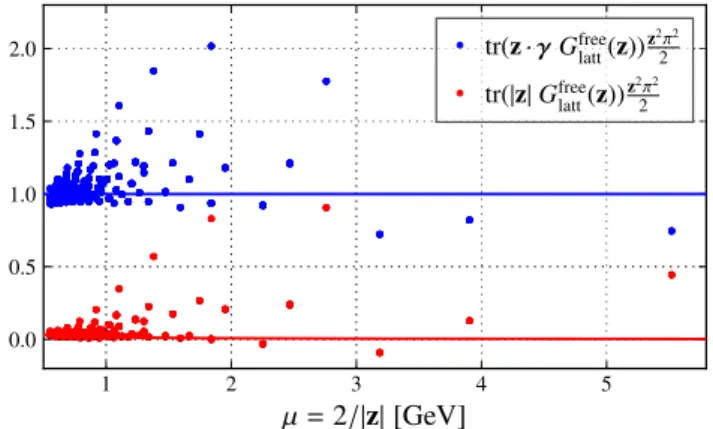
Fig. 4 The (free field) discretization effects of the Wilson propagator compared to the continuum expectation for the different Dirac structures
Fig. 5 Correction of discretization effects for the example of a fixed p·z=0.39 and|p| =1.08 GeV. Points with a correction larger than 10% (gray triangles) will be ignored in the analysis
ent. We find that the contribution from thechiral odd part, which removes the doublers and breaks chiral symmetry, can be of the same order of magnitude as the leading contribu- tion, cf. Fig.4. The “jumping” of the points nicely demon- strates the strong dependence of the lattice artifacts on the chosen direction. In particular the points along the axes [e.g., (1,0,0)] exhibit the largest discretization effects, while the points along the diagonal [e.g., (1,1,1)] are much better behaved. The large contribution of thechiral oddpart of the propagator is a peculiarity of using Wilson fermions. How- ever, the appearance of large discretization effects is probably a general feature of all coordinate space methods.
The appearance of large contributions from the chiral odd part of the propagator would lead to huge lattice artifacts in the correlator. However, the perturbative calculation shows that in the situation where the two currents are located sym- metrically with respect to the chosen origin, contributions
from the chiral even and the chiral odd parts of the prop- agator are nicely separated in some channels. For instance, for the scalar-pseudoscalar channel the contribution from the chiral even part (which is the one we are interested in) is real, while the chiral odd part appears only in the imaginary part.
Hence, we can choose to analyze only the part of the signal that does not contain the problematic contributions. Note, however, that the continuum expectation that either the real or the imaginary part (depending on which one corresponds to the chiral odd part) of the signal should be strongly sup- pressed isnot validfor the lattice data. Therefore, the correct identification of the relevant part of the signal is crucial.
We can now concentrate on the correction of the discretiza- tion effects in the chiral even part of the propagator (these correspond to the blue points in Fig.4). First and foremost we have decided to simply discard data points where the free field discretization effect is already larger than 10%, which mainly excludes very small distances (|z| 2a) and direc- tions along the lattice axes. For the remaining data points we use a correction factorccorr(z)determined such that the corrected propagator
Gcorrlatt(z)≡ccorr(z)Glatt(z) , (18) satisfies the condition
trc D
/zGcorrlatt(z) !
=trc D
/zGcont(z)
, (19)
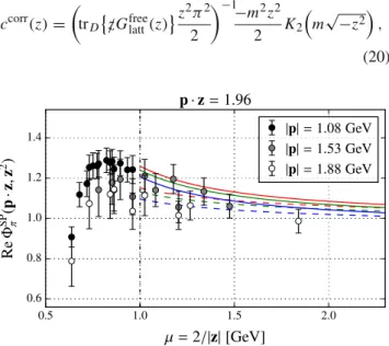
where the trace runs over Dirac and color indices. To zeroth order accuracy inαs (whereGlatt=Gfreelatt is the free propa- gator) this leads to
ccorr(z)=
trD
/zGfreelatt(z)z2π2 2
−1
−m2z2 2 K2
m√
−z2 , (20)
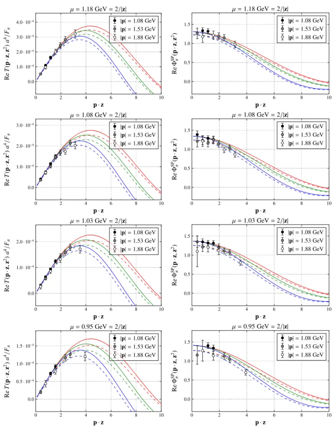
Fig. 6 The plots show our results for the scalar-pseudoscalar channel for different fixed values ofp·zand different pion momenta. The error- bars include the statistical error only. The solid/dashed lines correspond
to predictions taking into account/neglecting higher twist contributions for the different DA models (6). The color-coding is the same as in Fig.1
which corresponds to multiplying the blue data points in Fig.4with a factor such that one obtains the continuum result in the non-interacting case. Looking at Fig.5it is clear to the naked eye that this correction leads to a much smoother and less direction-dependent behavior of the data points.
4 Results
The gauge field ensemble used in this study has been gen- erated (by QCDSF / RQCD) with two mass-degenerate fla- vors of nonperturbatively improved Wilson fermions and the Wilson gluon action (ensemble IV in Ref. [39]). The dimen- sions of the lattice are 323×64 and the hopping parameter isκ = 0.13632. The coupling parameterβ = 5.29 trans- lates to the lattice spacinga ≈ 0.071 fm = (2.76 GeV)−1 and the pion mass has been determined in Ref. [40] to the valuemπ = 0.10675(59)/a ≈295 MeV. In order to get a reasonable overlap with the hadron state at large momentum, we have employed the momentum smearing technique (cf.
Ref. [2]) with APE smeared links [41].
The operator renormalization is performed as described in Ref. [38]. The local operators are renormalized nonper- turbatively in a RI-MOM scheme along with a subtraction of lattice artifacts in one-loop perturbation theory. The final conversion to the MS scheme employs 3 loop continuum perturbation theory. To be consistent, we use the Nf = 2 specific running ofαsin all perturbative calculations. To this end, we combine the results of Refs. [42] and [43] to obtain a value ofαs at 1000/a ≈2.76 TeV. From there we evolve it downwards using 5 loop running.
In Figs.6and7we confront the data points with predic- tions from continuum perturbation theory corresponding to the pion DAs shown in Fig.1. For all cases we show a version ignoring higher twist (i.e., twist 4) effects (dashed lines) and one including higher twist corrections (solid lines), where δ2π(1 GeV) = 0.2 GeV2 is set to the QCD sum rule esti- mate obtained in Ref. [44] (cf. also Ref. [45]). The error- bars only include the statistical error. It is clear that the systematic uncertainty is sizeable: in addition to discretiza- tion effects and higher order perturbative corrections there may be excited state contaminations and, possibly, finite vol- ume effects. Therefore, one should refrain from drawing any premature phenomenological conclusions. Nevertheless, the qualitative agreement found in Ref. [46] between our data points atμ =1.08 GeV and the results obtained using the quasi-DA method is encouraging.
In Fig.6, one immediately notices the higher twist effect, in particular for large distances, while the curves correspond- ing to the various DAs are hard to distinguish for small values ofp ·z. In Fig. 7 deviations from the asymptotic form are nicely visible at p · z 4. The latter region, however, can only be reached with larger hadron momenta,
since we are limited to perturbatively accessible values of
|z| = 2/μ 2 GeV−1 ≈ 5.5a. In Fig.7it becomes clear that our data points with|p| =1.88 GeV can already reach out into this region, but that one still needs higher statistics to be able to differentiate between different DA models.
5 Summary
In this work we have demonstrated that the coordinate space method for the determination of the pion DA proposed in Ref. [1] is promising, in particular as far as the statistical error is concerned. To this end, we have analyzed lattice data atmπ =295 MeV at a lattice spacing ofa=0.071 fm using dynamic Wilson fermions. We have shown that the large hadron momenta, which are a prerequisite of this method (and also for other related methods), lie just within the scope of the novel momentum smearing technique [2].
We have found particularly large discretization effects for directions along the coordinate axes, which are probably not specific to our calculation but will most likely occur also in other coordinate space calculations. Furthermore, we find that the chiral odd part of the quark propagator leads to large lattice artifacts. This contribution stems from the Wilson term in the propagator and is therefore a peculiarity of using Wil- son fermions. We have overcome this problem by analyz- ing the real part of the scalar-pseudoscalar channel, where only the chiral even part contributes. For the remaining dis- cretization effects stemming from the propagator, we have adopted the correction method described in Sect.3.3, which has reduced the anisotropy of the data considerably. However, observing large discretization effects on this single interme- diate lattice spacing shows that taking the continuum limit will be of vital importance, if one aims at achieving quanti- tative results in the future.
Unlike the Wilson line approach [5,16], the direction of the separation between the currents zcan be chosen arbi- trarily using our method. This enables us to realize a large number of different|z|andp·zvalues and also to study and minimize discretization effects. Intricacies related to the Wil- son line renormalization [11–18] are avoided entirely, and the possibility to vary the Dirac structures in the currents offers an additional handle on the higher-order perturbative correc- tions and higher twist effects.
In the near future we plan to investigate a new algorithm that may reduce the statistical uncertainties. We will also move to a smaller lattice spacing to enable the use of larger momenta|p| π/a (and therefore largerp·zvalues at a given scale μ = 2/|z| 1 GeV) along with distances
|z| a, which will reduce lattice artifacts.
Acknowledgements This work has been supported by the Deutsche Forschungsgemeinschaft (SFB/TRR-55) and the Studienstiftung des
Fig. 7 Results from the scalar-pseudoscalar channel for fixed values of the distancez2corresponding to perturbative scales aroundμ≈1GeV.
The errorbars only include the statistical error. Note that this comprises only a small subset of the available data. The left-hand-side plots dis- play the real part of the normalized matrix elementT(p·z,z2)/Fπ,
while those on the right-hand-side show the respective real part of ΦπSP(p·z,z2)defined in Eq. (4). At tree level and up to higher twist cor- rections, the latter correspond to the position space DA (5). Solid/dashed lines correspond to predictions that include/neglect higher twist contri- butions. The color-coding is the same as in Fig.1
deutschen Volkes. The analysis was carried out on the QPACE 2 [47]
Xeon Phi installation of the SFB/TRR-55 in Regensburg. We used a modified version of theChroma[48] software package along with the LibHadronAnalysislibrary and the multigrid solver implementation of Ref. [49] (see also Ref. [50]). We thank Daniel Richtmann for code development, discussions and software support.
Open Access This article is distributed under the terms of the Creative Commons Attribution 4.0 International License (http://creativecomm ons.org/licenses/by/4.0/), which permits unrestricted use, distribution, and reproduction in any medium, provided you give appropriate credit to the original author(s) and the source, provide a link to the Creative Commons license, and indicate if changes were made.
Funded by SCOAP3.
References
1. V.M. Braun, D. Müller, Eur. Phys. J. C 55, 349 (2008).
arXiv:0709.1348
2. G.S. Bali, B. Lang, B.U. Musch, A. Schäfer, Phys. Rev. D93, 094515 (2016).arXiv:1602.05525
3. G.S. Bali, V.M. Braun, M. Göckeler, M. Gruber, F. Hutzler, P. Kor- cyl, B. Lang, A. Schäfer, (RQCD). Phys. Lett. B774, 91 (2017).
arXiv:1705.10236
4. X. Ji, Phys. Rev. Lett.110, 262002 (2013).arXiv:1305.1539 5. J.-H. Zhang, J.-W. Chen, X. Ji, L. Jin, H.-W. Lin, Phys. Rev. D95,
094514 (2017).arXiv:1702.00008
6. U. Aglietti, M. Ciuchini, G. Corbò, E. Franco, G. Martinelli, L.
Silvestrini, Phys. Lett. B441, 371 (1998).arXiv:hep-ph/9806277 7. A. Abada, P. Boucaud, G. Herdoiza, J.P. Leroy, J. Micheli, O.
Pène, J. Rodríguez-Quintero, Phys. Rev. D64, 074511 (2001).
arXiv:hep-ph/0105221
8. W. Detmold, C.J.D. Lin, Phys. Rev. D 73, 014501 (2006).
arXiv:hep-lat/0507007
9. N.S. Craigie, H. Dorn, Nucl. Phys. B185, 204 (1981) 10. H. Dorn, Fortschr. Phys.34, 11 (1986)
11. T. Ishikawa, Y.-Q. Ma, J.-W. Qiu, S. Yoshida (2016).
arXiv:1609.02018
12. T. Ishikawa, Y.-Q. Ma, J.-W. Qiu, S. Yoshida, PoSLATTICE2016, 177 (2016).arXiv:1703.08699
13. G.C. Rossi, M. Testa, Phys. Rev. D 96, 014507 (2017).
arXiv:1706.04428
14. X. Ji, J.-H. Zhang, Y. Zhao, Nucl. Phys. B 924, 366 (2017).
arXiv:1706.07416
15. X. Ji, J.-H. Zhang, Y. Zhao (2017).arXiv:1706.08962
16. K. Orginos, A.V. Radyushkin, J. Karpie, S. Zafeiropoulos, Phys.
Rev. D96, 094503 (2017).arXiv:1706.05373
17. C. Alexandrou, K. Cichy, M. Constantinou, K. Hadjiyiannakou, K. Jansen, H. Panagopoulos, F. Steffens, Nucl. Phys. B923, 394 (2017).arXiv:1706.00265
18. J. Green, K. Jansen, F. Steffens (2017).arXiv:1707.07152 19. X. Ji, Sci. China Phys. Mech. Astron. 57, 1407 (2014).
arXiv:1404.6680
20. V.M. Braun, P. Górnicki, L. Mankiewicz, Phys. Rev. D51, 6036 (1995).arXiv:hep-ph/9410318
21. Y.-Q. Ma, J.-W. Qiu (2014).arXiv:1404.6860
22. Y.-Q. Ma, J.-W. Qiu, Int. J. Mod. Phys. Conf. Ser.37, 1560041 (2015).arXiv:1412.2688
23. Y.-Q. Ma, J.-W. Qiu, Phys. Rev. Lett. 120, 022003 (2018).
arXiv:1709.03018
24. K.-F. Liu, S.-J. Dong, Phys. Rev. Lett. 72, 1790 (1994).
arXiv:hep-ph/9306299
25. A.V. Radyushkin, Phys. Rev. D 96, 034025 (2017).
arXiv:1705.01488
26. A.V. Radyushkin, Phys. Rev. D 95, 056020 (2017).
arXiv:1701.02688
27. K.G. Chetyrkin, A. Maier, Nucl. Phys. B 844, 266 (2011).
arXiv:1010.1145
28. B. Aubert et al., (BaBar), Phys. Rev. D 80, 052002 (2009).
arXiv:0905.4778
29. S. Uehara et al., (Belle), Phys. Rev. D 86, 092007 (2012).
arXiv:1205.3249
30. S.S. Agaev, V.M. Braun, N. Offen, F.A. Porkert, Phys. Rev. D83, 054020 (2011).arXiv:1012.4671
31. S.V. Mikhailov, A.V. Pimikov, N.G. Stefanis, Phys. Rev. D 93, 114018 (2016).arXiv:1604.06391
32. T. Horn, C.D. Roberts, J. Phys. G 43, 073001 (2016).
arXiv:1602.04016
33. V.M. Braun, I.E. Filyanov, Z. Phys. C48, 239 (1990)
34. P. Ball, V.M. Braun, A. Lenz, JHEP 05, 004 (2006).
arXiv:hep-ph/0603063
35. S.V. Mikhailov, A.V. Radyushkin, Nucl. Phys. B273, 297 (1986) 36. D. Müller, Phys. Rev. D49, 2525 (1994)
37. V.M. Braun, A.N. Manashov, S. Moch, M. Strohmaier, JHEP06, 037 (2017).arXiv:1703.09532
38. M. Göckeler et al. (QCDSF/UKQCD), Phys. Rev. D 82, 114511 (2010). [Erratum: Phys. Rev. D 86, 099903 (2012)], arXiv:1003.5756
39. G.S. Bali, S. Collins, B. Gläßle, M. Göckeler, J. Najjar, R.H. Rödl, A. Schäfer, R.W. Schiel, A. Sternbeck, W. Söldner, Phys. Rev. D 90, 074510 (2014).arXiv:1408.6850
40. G.S. Bali et al., Phys. Rev. D91, 054501 (2015).arXiv:1412.7336 41. M. Falcioni, M.L. Paciello, G. Parisi, B. Taglienti, Nucl. Phys. B
251, 624 (1985)
42. P. Fritzsch, F. Knechtli, B. Leder, M. Marinkovic, S. Schae- fer, R. Sommer, F. Virotta, Nucl. Phys. B 865, 397 (2012).
arXiv:1205.5380
43. G.S. Bali et al., (QCDSF), Nucl. Phys. B 866, 1 (2013).
arXiv:1206.7034
44. V.A. Novikov, M.A. Shifman, A.I. Vainshtein, M.B. Voloshin, V.I.
Zakharov, Nucl. Phys. B237, 525 (1984)
45. V.M. Braun, A. Khodjamirian, M. Maul, Phys. Rev. D61, 073004 (2000).arXiv:hep-ph/9907495
46. J. W. Chen, L. Jin, H. W. Lin, A. Schäfer, P. Sun, Y. B. Yang, J. H.
Zhang, R. Zhang, Y. Zhao, (LP3) (2017).arXiv:1712.10025 47. P. Arts et al., PoSLATTICE2014, 021 (2015).arXiv:1502.04025 48. R.G. Edwards, B. Joó, (SciDAC/LHPC/UKQCD). Nucl. Phys.
Proc. Suppl140, 832 (2005).arXiv:hep-lat/0409003
49. S. Heybrock, M. Rottmann, P. Georg, T. Wettig, PoS LAT- TICE2015, 036 (2015).arXiv:1512.04506
50. A. Frommer, K. Kahl, S. Krieg, B. Leder, M. Rottmann, SIAM J.
Sci. Comput.36, A1581 (2014).arXiv:1303.1377