I N V E S T I G AT I O N O F D R I Z Z L E O N S E T I N L I Q U I D C L O U D S U S I N G G R O U N D B A S E D A C T I V E A N D PA S S I V E R E M O T E S E N S I N G I N S T R U M E N T S i n a u g u r a l – d i s s e r t a t i o n zur erlangung des d

I N V E S T I G AT I O N O F D R I Z Z L E O N S E T I N L I Q U I D C L O U D S U S I N G G R O U N D B A S E D A C T I V E A N D PA S S I V E R E M O T E S E N S I N G

I N S T R U M E N T S

i n a u g u r a l – d i s s e r t a t i o n z u r

e r l a n g u n g d e s d o k t o r g r a d e s

d e r m at h e m at i s c h - nat u r w i s s e n s c h a f t l i c h e n f a k u ltät d e r u n i v e r s i tät z u k ö l n

v o r g e l e g t v o n

C L A U D I A A C Q U I S TA PA C E au s p i s a , i ta l i e n

k ö l n , 1 4 . n ov e m b e r 2 0 1 6

PD Dr. Ulrich Löhnert Prof. Dr. Roel Neggers Prof. Dr. Pavlos Kollias

ta g d e r m ü n d l i c h e n p r ü f u n g :

23 . 01 . 2017

Considerate la vostra semenza:

fatti non foste a viver come bruti ma per seguir virtute e canoscenza

— Dante Alighieri —

Firenze, 1 June 1265 – Ravenna, 14 September 1321

Dedicated to my family

A B S T R A C T

One of the major challenges of climate prediction is a correct repre- sentation of the interactions among aerosols, clouds and precipitation.

Aerosols have a strong impact on the life cycle of boundary layer clouds, which are known to significantly influence the energy avail- able to the Earth-Atmosphere system. Specifically, drizzle formation in low-level clouds, which has been shown to depend on aerosol con- centration (second indirect aerosol effect), determines cloud life time.

In models, the transition from liquid cloud to precipitation must be parameterized by the so-called autoconversion process. Different pa- rameterizations of autoconversion have been developed, whereby the corresponding transition rates differ of up to one order of magnitude.

Even observations of this microphysical process are very challeng- ing. Satellite observations have been exploited in the past to evaluate different autoconversion schemes but one of the main reasons for the encountered differences between models and observations was the poor representation of the vertical cloud structure in the satellite ob- servations. In this context, ground-based cloud observations present a unique tool to provide observational constraints for model parame- terization development by exploiting their highly temporally and spa- tially resolved profiling capability. In recent years, new ground-based techniques exploiting higher moments of the cloud radar Doppler spectrum (the skewness, in particular) have been successfully applied for the detection of drizzle onset in maritime clouds.

In this thesis, a new, extended ground-based dataset for continental liquid clouds is exploited in order to assess the potential for early drizzle detection. For this purpose, ground-based observations of liq- uid water path and of the cloud radar Doppler moments reflectivity, mean Doppler velocity, spectral width and skewness have been syn- ergetically exploited. It has been found that skewness detects drizzle formation at an earlier stage than the other radar moments.

The different observational variables have been used for the de- velopment of a drizzle probability index (DI) to improve currently available drizzle classification schemes, i.e. Cloudnet. The DI repre- sents the probability of each cloud radar bin to contain drizzle. In comparison to the Cloudnet classification, case studies show that the DI detects earlier stages of drizzle formation and eliminates falsely detected, inconsistent time-height drizzle structures. However, due to the presence of turbulence, the DI sometimes falsely attribute drizzle to a pixel.

In order to understand how turbulence can impact radar Doppler measurements and also in order to optimize the radar measurement

v

settings for the purpose of drizzle detection, sensitivity studies on integration time, spectral resolution and radar antenna beam width have been conducted using raw radar data and a forward radar simu- lator. It has been found that integration times no longer than 2 seconds should be used for drizzle detection and that the spectral resolution obtained with the fast Fourier transform (FFT) using 256 FFT points resolves the characteristics of the Doppler spectrum with sufficient accuracy. Also, simulations showed that smaller beam widths are beneficial for drizzle detection and that turbulence is responsible for an increase of spectral width and a reduction of observed skewness values.

Finally, a microphysical interpretation of the skewness signal is pro- vided by comparing the simulations of drizzle formation from a 1 D steady-state binned microphysical model to observations. The forward simulated vertical profiles of skewness based on the modeled cloud drop and drizzle size distributions strongly depend on the applied au- toconversion parameterization. A validation of the different schemes indicates that the scheme from Seifert et al. ( 2010 ) best matches the ob- servations of reflectivity and skewness. The comparison also suggests that the modeled autoconversion rates tend to produce large drizzle too fast and too early for continental liquid clouds. This first model comparison thus demonstrates that ground-based cloud radar obser- vations, particularly skewness, can be used for testing autoconversion parameterizations.

The dataset and the results of this work constitute a unique basis for evaluating model outputs, e.g. in a next step the results of large eddy simulations, and for carrying out additional process studies to refine for example the drizzle detection criterion. Also, this data set could be exploited for future validations of satellite products, e.g.

of EarthCARE. This thesis hence shows how ground-based cloud

radar observations can be optimally exploited to better understand

the autoconversion process and also represents an important step

forward in bringing observations of drizzle and modeling together.

Z U S A M M E N FA S S U N G

Eine der größten Herausforderungen in der Klimavorhersage ist die korrekte Darstellung der Wechselwirkungen zwischen Aerosolen, Wol- ken und Niederschlag. Aerosole wirken sich stark auf den Lebenszy- klus von Grenzschichtwolken aus, welche wiederum signifikant die verfügbare Energie im System Erde/Atmosphäre beeinflussen. Insbe- sondere bestimmt die Bildung von Niesel, welche von der Aerosolkon- zentration abhängt (zweiter indirekter Aerosoleffekt), die Lebenszeit niedriger Wolken. In Modellen muss der Übergang von Wolkentrop- fen zu Niederschlag durch den sogenannten Autokonversionsprozess parametrisiert werden. Verschiedene Parametrisierungen der Auto- konversion wurden entwickelt, wobei sich die entsprechenden Über- gangsraten bis zu einer Größenordnung unterscheiden. Auch Beob- achtungen dieses mikrophysikalischen Prozesses stellen eine große Herausforderung dar. In der Vergangenheit wurden von Satelliten aus durchgeführte Messungen verwendet, um verschiedene Autokon- versionsschemata zu evaluieren. Einer der Hauptgründe für die Un- terschiede zwischen den Modellen und Satellitenbeobachtungen war jedoch die schlechte vertikale Auflösung der Wolkenstruktur in den Beobachtungen. In diesem Zusammenhang bieten bodengebundene Wolkenbeobachtungen aufgrund ihrer hohen zeitlichen und räum- lichen Auflösung eine einzigartige Beobachtungsgrundlage, um Pa- rametrisierungen für Modelle zu entwickeln. In den letzten Jahren wurden bodengebundene Messverfahren, die höhere Momente des Wolkenradarspektrums (insbesondere die Schiefe) ausnutzen, erfolg- reich angewendet, um das Einsetzen von Niesel in maritimen Wol- ken zu detektieren. In dieser Arbeit wird ein neuer, umfassender Da- tensatz bodengebundender Beobachtungen von kontinentalen Was- serwolken verwendet, um das Potential zur frühzeitigen Detektion von Niesel abzuschätzen. Zu diesem Zweck wurden bodengebunde- ne Beobachtungen des Flüssigwasserpfades und der Dopplermomen- te eines Wolkenradars (Reflektivität, mittlere Dopplergeschwindig- keit, spektrale Breite und Schiefe) synergetisch ausgewertet. Es hat sich dabei gezeigt, dass die Schiefe im Vergleich zu den anderen Ra- darmomenten Nieselbildung in einem früheren Stadium detektiert.

Die verschiedenen Beobachtungsgrößen wurden zur Entwicklung ei- nes Nieselindizes (DI) herangezogen, um die zurzeit bestehenden Niesel-Klassifikationsschemata, z. B. Cloudnet, zu verbessern. Der DI beschreibt die Wahrscheinlichkeit, dass in dem jeweiligen betrachte- ten Wolkenradarvolumen Niesel vorkommt. Fallstudien zeigen, dass im Vergleich zu der Cloudnetklassifikation der DI früheren Stadien der Nieselbildung detektiert. Der DI entfernt zudem durch Cloudnet fälschlicherweise detektierte, d.h. in Zeit und Höhe inkonsistente, Nie-

vii

selstrukturen. Das Auftreten von Turbulenz kann jedoch manchmal

dazu führen, dass der DI irrtümlich Niesel detektiert. Um zu verste-

hen, welchen Einfluss Turbulenz auf die Radar-Dopplermomente hat

und um die Messeinstellungen des Radars für die Detektion von Nie-

sel zu optimieren, wurden Sensitivitätsstudien hinsichtlich Integra-

tionszeit, spektraler Auflösung und Antennenöffnungswinkel durch-

geführt. Dazu wurden die unbearbeiteten, ursprünglichen Radarda-

ten und ein Radar-Vorwärtssimulator verwendet. Es hat sich gezeigt,

dass die Eigenschaften des Dopplerspektrums mit einer ausreichen-

den Genauigkeit wiedergegeben werden, wenn die Integrationszei-

ten nicht länger als 2 Sekunden sind. Zudem reicht es, eine spektra-

le Auflösung zu wählen, die mit einer Fast-Fourier-Transformation

(FFT) mit 256 FFT-Punkten erzeugt wird. Darüber hinaus haben die

Simulationen gezeigt, dass kleinere Antennen-öffnungswinkel vor-

teilhaft für die Detektion von Niesel sind und dass Turbulenz die

spektrale Breite vergrößert und die Schiefe des Dopplerspektrums ver-

kleinert. Abschließend, wird eine mikrophysikalische Interpretation

des Signals in der Schiefe gegeben, indem Simulationen von Niesel-

bildung basierend auf einem sogenannten “ 1 D steady-state binned

microphysical”-Modell mit Beobachtungen verglichen werden. Die

Vertikalprofile der Schiefe, die auf Vorwärtssimulationen der model-

lierten Wolkentropfen- und Nieselgrößenverteilungen basieren, hän-

gen stark von der jeweils verwendeten Autokonversionsparametrisie-

rung ab. Eine Validierung der verschiedenen Schemata hat gezeigt,

dass das Schema von Seifert et al. ( 2010 ) am besten die Beobachtungen

der Reflektivität und Schiefe wiedergibt. Der Vergleich legte außer-

dem nahe, dass die modellierten Autokonversionsraten dazu neigen,

große Nieseltropfen in kontinentalen Flüssigwasserwolken zu schnell

und zu früh zu erzeugen. Dieser erste Modellvergleich zeigt daher,

dass bodengebundene Wolkenradarbeobachtungen, insbesondere die

Schiefe, genutzt werden können, um Autokonversionsparametrisie-

rungen zu testen. Der Datensatz und die Ergebnisse dieser Arbeit

bilden eine einzigartige Grundlage für die Evaluierung von Modeller-

gebnissen, z.B. in einem nächsten Schritt die Ergebnisse von Large-

Eddy-Simulationen, und für das Durchführen weiterer Prozessstudien

um z.B. das Kriterium zur Nieseldetektion zu verfeinern. Außerdem

kann dieser Datensatz zukünftig genutzt werden um Satellitenpro-

dukte, z.B. von EarthCARE, zu validieren. Diese Arbeit zeigt, wie

bodengebundene Wolkenradarbeobachtungen optimal genutzt wer-

den können, um den Prozess der Autokonversion besser zu verstehen

und macht zudem einen weiteren wichtigen Schritt hinsichtlich des

Zusammenführens von Nieselbeobachtungen und Modellen.

C O N T E N T S

i i n t r o d u c t i o n 1 1 m o t i vat i o n 3

2 s c i e n t i f i c b a c k g r o u n d 11

2 . 1 Warm rain processes: theoretical perspective 11 2 . 1 . 1 The theory of warm rain formation 11

2 . 1 . 2 The problem of the initiation of coalescence 16 2 . 2 Microphysical processes in models 17

2 . 3 Measuring liquid clouds and light precipitation 25 2 . 3 . 1 Microwave radiometer 25

2 . 3 . 2 Cloud radar 26

2 . 4 Observations of drizzle onset 35 ii t o o l s a n d d ata 41

3 i n s t r u m e n t s a n d m e t h o d s 43 3 . 1 HATPRO Microwave radiometer 43 3 . 2 35 GHz Cloud radar JOYRAD-35 46 3 . 3 Ceilometer 51

3 . 4 Cloudnet target categorization 51

3 . 5 Passive and Active Microwave Transfer (Pamtra) for- ward model 54

4 d ata b a s e f o r i d e n t i f y i n g p r e c i p i tat i o n 59 4 . 1 Liquid clouds at JOYCE 59

4 . 2 Assessment of drizzle detection by Cloudnet 66 4 . 3 Extended analysis of drizzling/non-drizzling cloud prop-

erties 68

4 . 3 . 1 Statistical properties 68

4 . 3 . 2 Dataset characterization in terms of radar Doppler moments and LWP 70

iii d e t e c t i n g d r i z z l e w i t h s k e w n e s s 75

5 m i c r o p h y s i c a l i n t e r p r e tat i o n o f s k e w n e s s 77 5 . 1 The concept: interpreting the skewness signal 77 5 . 2 Observations from two case studies 78

5 . 3 Description of the model 80

5 . 4 Confronting model and observations 85

5 . 5 Interpretation of skewness in terms of drizzle droplet size 95

5 . 6 Conclusions and summary of the results 97

6 o p t i m i z i n g o b s e r vat i o n s o f d r i z z l e o n s e t w i t h m m - wav e l e n g t h r a d a r s 99

6 . 1 Motivation and concept of the study 99

ix

6 . 2 Methodology for the processing of the IQ raw radar data 101

6 . 3 IQ raw radar dataset 102

6 . 4 Impact of integration time and spectral resolution on the observations 104

6 . 4 . 1 Moments time series 105

6 . 4 . 2 Impact of spectral resolution 107

6 . 4 . 3 Probability density functions for each combina- tion of settings 110

6 . 5 Simulation framework: statistics and impact of hardware parameters 113

6 . 5 . 1 Simulation statistics for early stage and mature drizzle cases 116

6 . 5 . 2 Effects of turbulence and varied antenna beamwidth 119 6 . 6 Conclusion and summary of main results 120

iv e x p l o i t m e n t o f s k e w n e s s f o r o p e r at i o na l a p p l i - c at i o n s 123

7 r e f i n e m e n t o f d r i z z l e d e t e c t i o n 125

7 . 1 Distributions of observed variables for drizzling/ non- drizzling clouds 125

7 . 2 The algorithm for calculating the drizzle index 132 7 . 3 Performance on case studies at high resolution 134

7 . 3 . 1 Drizzling case study of the 5 Jan 2013 134 7 . 3 . 2 Drizzling case study of the 9 October 2013 137 7 . 3 . 3 Transition case study of the 31 July 2013 139 7 . 3 . 4 Non-drizzling case study of the 1 October 2013 142 7 . 4 Comparison with Cloudnet 147

7 . 5 Conclusions and summary of main results 148 8 c o n c l u s i o n s a n d o u t l o o k 151

a b b r e v i at i o n s 157

s y m b o l s 161

b i b l i o g r a p h y 163

L I S T O F F I G U R E S

Figure 1 . 1 Increase of CO

concentration in the period 1958 -

2016 . 3

Figure 1 . 2 Change of the equilibrium temperature as predicted by 12 GCMs in the scenario of doubling the CO

concentration (from Dufresne and Bony ( 2008 )). 4 Figure 2 . 1 Example of cloud drop size distribution (from Wal-

lace and Hobbs ( 2006 )). 12

Figure 2 . 2 Collision efficiency for pairs of drops. 14 Figure 2 . 3 Microphysical growth rates for condensation and

collision-coalescence. 16

Figure 2 . 4 Effect of GCCN on precipitation rates in ECHAM 5 (from Posselt and Lohmann ( 2008 )). 17 Figure 2 . 5 Characteristics times and scales of models. 18 Figure 2 . 6 Collision processes in bulk schemes (from Khain

et al. ( 2015 )). 20

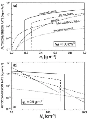
Figure 2 . 7 Comparison of autoconversion rates (from Wood ( 2005 b)) 24

Figure 2 . 8 Absorption coefficient for atmospheric gases as a function of frequency. 26

Figure 2 . 9 Dielectric constant for water in the range of fre- quencies 1 − 50 GHz. 30

Figure 2 . 10 Illustration of the standard procedure for deriv- ing radar Doppler spectra from raw I/Q time se- ries. 33

Figure 2 . 11 Example of an observed cloud radar Doppler spec- trum. 34

Figure 2 . 12 Explanation of skewness as tracer for drizzle on- set. 36

Figure 2 . 13 Skewness as a function of reflectivity for a marine stratus cloud (from Luke and Kollias ( 2013 )). 39 Figure 2 . 14 Schematic representation of the dynamical induced

skewness signal (from Luke and Kollias ( 2013 )) 40 Figure 3 . 1 EM extinction in microwave region 45

Figure 3 . 2 Example of fit to the power law

for the energy spectrum E(f). 49

Figure 3 . 3 Case study for calculation of . 50 Figure 3 . 4 Distribution of . 50

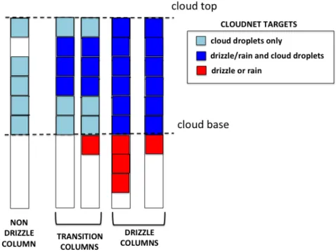
Figure 3 . 5 Drizzling, non-drizzling and transition vertical columns based on Cloudnet. 53

Figure 4 . 1 Precipitation amount at JOYCE between March 2012 and August 2013 . 60

xi

Figure 4 . 2 LWP statistics of JOYCE observation and COSMO- DE for the period mar 2012 -mar 2013 . 61 Figure 4 . 3 Geometrical thickness statistics of JOYCE observa-

tion and COSMO-DE for the period March 2012 - March 2013 . 62

Figure 4 . 4 2 D probability of precipitation for JOYCE data for the period March 2012 - March 2013 . 63 Figure 4 . 5 2D probability of precipitation for COSMO-DE data

for the period March 2012 -March 2013 . 63

Figure 4 . 6 Example of boundary layer non-drizzling cloud. 64 Figure 4 . 7 Example of stratocumulus non-drizzling cloud. 64 Figure 4 . 8 Example of boundary layer drizzling cloud. 65 Figure 4 . 9 Example of stratocumulus drizzling cloud. 66 Figure 4 . 10 Example of physical inconsistency in Cloudnet tar-

get categorization. 67

Figure 4 . 11 Analysis of the inconsistency in Cloudnet target categorization. 68

Figure 4 . 12 Z

mean values distributed as a function of dis- tance from clout top and LWP. 71

Figure 4 . 13 V

mean values distributed as a function of dis- tance from clout top and LWP. 71

Figure 4 . 14 S

mean values distributed as a function of dis- tance from cloud top and LWP. 73

Figure 4 . 15 S

mean values distributed as a function of distance from cloud top and LWP. 73

Figure 5 . 1 Z

for the case of the the 31 July 2013 , from 9 . 2 UTC to 10.0 UTC. 79

Figure 5 . 2 S

field selected by the skewness mask for the case of the the 31 July 2013 , from 9 . 2 UTC to 10 . 0 UTC. 80 Figure 5 . 3 V

for the case of the the 31 July 2013 , from 9.2

UTC to 10 . 0 UTC. 81

Figure 5 . 4 Scheme representing the working principle of the steady state bin microphysical model employed in this study. 82

Figure 5 . 5 LWC profiles of model and observations. 83 Figure 5 . 6 Cloud and drizzle drop size distributions. 84 Figure 5 . 7 Example of autoconversion rates profiles (left) and

accretion rates profiles (right) for the different schemes. 85 Figure 5 . 8 Comparison of Z

profiles derived using different

N. 87

Figure 5 . 9 Comparison of Z

profiles derived using different LWC profiles. 88

Figure 5 . 10 Comparison of Z

profiles derived using different initial drizzle sizes. 89

Figure 5 . 11 Comparison of mean observed and simulated V

profiles. 91

List of Figures xiii

Figure 5 . 12 Comparison of mean observed and simulated S

profiles. 92

Figure 5 . 13 Comparison of mean observed and simulated S

profiles. 93

Figure 5 . 14 V

as a function of S

for the mature drizzle devel- opment case study. 96

Figure 5 . 15 Relation between skewness and equivalent drizzle size for observations. 97

Figure 5 . 16 Relation between skewness and equivalent drizzle size for model data. 98

Figure 6 . 1 Overview of the non drizzle case study of the 20 November 2014 . 103

Figure 6 . 2 Overview of the drizzle case study of the 24 June 2015 . 104

Figure 6 . 3 Time series of Doppler moments for different inte- gration times for the drizzling case study. 105 Figure 6 . 4 Time series of Doppler moments for different inte-

gration times for the non-drizzle case study. 106 Figure 6 . 5 Impact of spectra resolution for non drizzling case. 108 Figure 6 . 6 Impact of spectra resolution for drizzle case. 109 Figure 6 . 7 PDFs of the moments for the non-drizzling case. 110 Figure 6 . 8 PDFs of radar moments for drizzling case. 112 Figure 6 . 9 DSDs used in the simulations of IQ experiment. 114 Figure 6 . 10 Comparison between simulated and observed spec-

tra. 115

Figure 6 . 11 Distribution of simulated moments for drizzle DSD with R

= 20µm and r

= 2.0%. 116 Figure 6 . 12 Distribution of simulated moments for drizzle DSD

with R

= 30µ m and r

= 0 . 5 %. 117 Figure 6 . 13 Distribution of a selected fingerprint of drizzle de-

velopment. 118

Figure 6 . 14 Simulated skewness as a function of r

. 119 Figure 7 . 1 Z

distribution for the whole dataset. 127 Figure 7 . 2 V

distribution for the whole dataset. 127 Figure 7 . 3 S

distribution for the whole dataset. 128 Figure 7 . 4 S

distribution for the whole dataset. 129 Figure 7 . 5 2D histogram for Z

and S

for non-drizzling pix-

els. 129

Figure 7 . 6 2D histogram for Z

and S

for drizzling pixels. 130 Figure 7 . 7 2D histogram for Z

and S

for transition pix-

els. 131

Figure 7 . 8 LWP distribution for the whole dataset. 131 Figure 7 . 9 Geometrical thickness distribution for the whole

dataset. 132

Figure 7 . 10 DI index time height plot for the drizzle case of 5

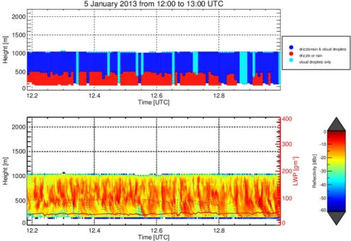
January 2013 . 135

case of the January .

Figure 7 . 12 Overview of the variables in all pixels which have a DI = 0.4 for the drizzle case of the 5 January 2013 . 137

Figure 7 . 13 DI index time height plot for the drizzle case of the 9 October 2013 . 138

Figure 7 . 14 Distribution of DI values obtained for the drizzling case of the 9 October 2013 . 138

Figure 7 . 15 Normalized distributions of Z

, V

, S

, S

and LWP for various DI values for the case study of the 09 October 2013 , between 1.2 and 2.0 UTC. 140 Figure 7 . 16 DI index time height plot for the drizzle case of 31 st

July 2013 . 141

Figure 7 . 17 Distribution of DI values obtained for the drizzling case of the 31 July 2013 . 142

Figure 7 . 18 Normalized distributions of Z

, V

, S

, S

and LWP for various DI values for the case study of the 31 July 2013 , between 9 . 2 and 10 . 0 UTC. 143 Figure 7 . 19 DI index time height plot for the non-drizzle case

of the 1 October 2013 . 144

Figure 7 . 20 Normalized DI distribution for the case of the 1 October 2013 . 145

Figure 7 . 21 Normalized distributions of Z

, V

, S

, S

and LWP for various DI values for the case study of the 1 October 2013 , between 5 . 2 and 6 . 0 UTC. 146 Figure 7 . 22 Comparison between Cloudnet and DI for the driz-

zle case of the 13 July 2013 . 148

L I S T O F TA B L E S

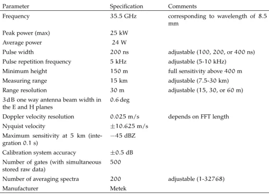
Table 3 . 1 Current radar settings for JOYRAD-35 system at JOYCE, Jülich (DE). 47

Table 3 . 2 Parameters provided to PAMTRA for simulat- ing JOYRAD-35 observations 57

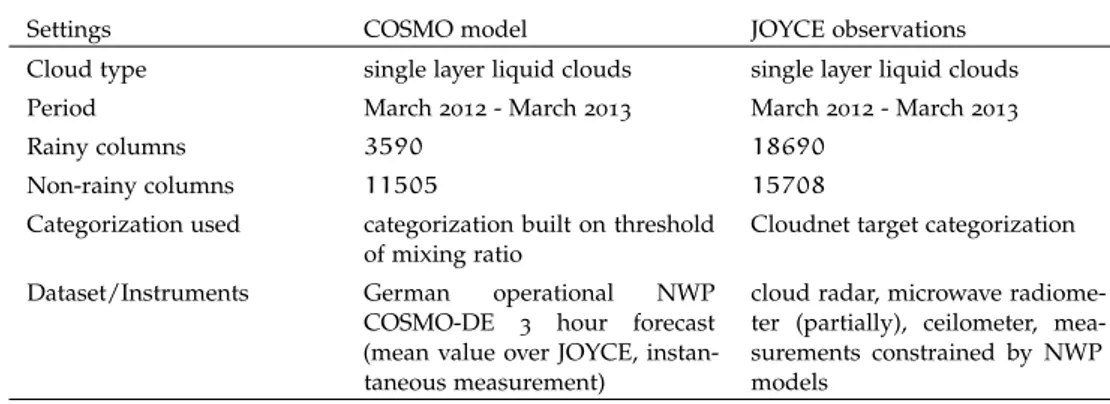
Table 4 . 1 COSMO model and observations characteris- tics for the statistical comparison. 62 Table 4 . 2 Statistical properties of the ensemble of case

studies used. 69

Table 6 . 1 Radar settings for operating MIRA METEK sys- tems. 100

Table 6 . 2 Number of averaged spectra for every integra- tion time. 101

xiv

List of Tables xv

Table 6 . 3 Bias and standard deviation of moments de- rived with different spectral resolutions for the drizzle case. 107

Table 6 . 4 Bias and standard deviation of moments de- rived with different spectral resolutions for the non-drizzle case. 107

Table 6 . 5 Mean values of moments distributions: 20 Novem- ber 2014 . 111

Table 6 . 6 Mean values of moments distributions: 24 June 2015 . 112

Table 7 . 1 Derivation of flag for every variable in the χ

test. 133

Table 7 . 2 Example of classification array for every pixel. 134

Part I

I N T R O D U C T I O N

If I have seen further than others, it is by standing upon the shoulders of giants.

Isaac Newton

Woolsthorpe-by-Colsterworth, 25 December 1642 –

London, 20 March 1727

1

M O T I VAT I O N

In the month of September 2016 , the CO

concentration in the atmo- sphere for the first time exceeded the value of 400 ppm and it will remain above that value permanently (Fig. 1 . 1 ) (Betts et al., 2016 ).

CO

is one of the substances that are called drivers of climate change, because it alters the Earth’s energy budget with its increasing concen-

tration.

science basis of th IPCC report of2013:

http://www.

climatechange2013.

org/

Figure1.1:CO₂ concentrations measured at Mauna Loa station in the period 1958-2016 (produced by Ed Hawkins and available at http://www.climate-lab-book.ac.uk/

spirals/), inspired byBetts et al.(2016). The spiral draws the evolution in time of theCO2concentration, starting from320ppm. Values measured in the preindus- trial era (1800) were of280ppm (not shown here).

Radiative forcing quantifies the change in energy fluxes caused by the change of the drivers in the period of time from 1750 to present time. A positive forcing leads to surface warming (IPCC, 2014 ). The IPCC ( 2014 ) states that the total radiative forcing of the planet is pos-

3

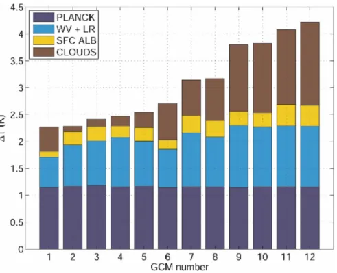
Figure1.2: Change of average Earth temperature as predicted by12GCMs in the scenario of doubling theCO2concentration (fromDufresne and Bony(2008)). Impact of dif- ferent feedbacks is shown in different colors: the Planck feedback gives the climate sensitivity in absence of variations of the climate system, the water vapour feedback accounts for the change in longwave radiation caused by water vapour, the surface albedo feedback accounts for change of the albedo at the surface and the cloud feedback considers the effects of clouds.

itive and the largest contribution to it comes from the increase of the concentration of atmospheric CO

. Plenty of observations show evidences that the climate is changing. General circulation models (GCMs) have been developed to forecast the average increase in tem- perature due to such forcings in future climate scenarios.

The overall response of a climate system to a change in radiative forcing, for example an increase of CO

, is defined as climate sensitiv- ity. Processes that change the climate sensitivity are called feedbacks (Dal Gesso, 2015 ). Figure 1 . 2 shows the change of the surface temper- ature for a scenario of doubling CO

(Dufresne and Bony, 2008 ) for 12 different GCMs. The order of uncertainty among the predictions of different models is comparable to the variation of temperature it- self. Moreover, from the decomposition of the feedbacks, the main contribution to this uncertainty comes from the cloud feedback, iden- tified by Bony and Dufresne ( 2005 ) to be caused by boundary layer clouds. These are clouds that form at the top of the atmospheric layer (boundary layer) which is affected by the interactions with the surface.

In fact, low level liquid clouds (boundary layer clouds and stratocu-

muli) represent one of the main causes of the spread among different

m o t i vat i o n 5

model climate predictions (Bony et al., 2006 ). Mainly, this is because these clouds, so called warm because of the absence of ice, reduce the solar energy absorbed by the Earth system in the shortwave re- gion and lead in general to a cooling effect with respect to cloud free conditions (Randall et al., 1984 ). The radiative properties of warm clouds are defined by their number concentration and by the hori- zontal and vertical distribution of cloud liquid water content (Weber and Quaas, 2012 ). Both these cloud properties are strictly connected with the aerosol presence. In fact, aerosols can have a strong impact on warm clouds properties in mainly two ways. An increase in the number of aerosol particles can produce a higher droplet total number concentration (N) and hence a higher cloud albedo, if the amount of liquid water in the cloud is considered constant (first indirect effect) (Twomey, 1977 ). The same increase in aerosol concentration can inhibit the coalescence between droplets and hence suppresses the precipita- tion (second indirect effect) (Albrecht, 1989 ). However, cloud systems exhibit a high variability caused by dynamics and it is hence very dif- ficult to attribute changes in precipitation to aerosol perturbations (Sorooshian et al., 2009 ).

In warm clouds, the second aerosol indirect effect can inhibit driz- zle production and change cloud properties, lifetime and extent, with consequences also on the cloud cover (Mann et al., 2014 ). Various modeling studies show that high concentrations of cloud condensa- tion nuclei (CCNs) cause a reduction in drizzle formation in warm clouds (Wang et al., 2011 b,a). The same effect was also present in field campaigns conducted to study marine stratocumuli (Wood, 2005 a; Lu et al., 2007 , 2009 ). Regarding the first aerosol indirect effect, satellite datasets have been used to quantify the impact of higher CCN con- centrations on cloud droplet size (Lebsock et al., 2008 ) and also to estimate the cloud albedo effect (Forster et al., 2007 ; L’Ecuyer et al., 2009 ). Modelling cloud albedo is also linked to the representation of drizzle because more drizzle is generally associated with open cells, while overcasted areas of stratocumuli often show light drizzle. There- fore a proper description of vertical and horizontal distributions of cloud liquid water connected with drizzle formation is needed also for properly simulating other characteristics, i.e. cloud albedo, cloud fraction and radiative forcing of boundary layer clouds (Stevens et al., 2005 ; Ahlgrimm and Forbes, 2014 ).

In GCMs, the rate at which precipitation is produced is controlled

by the autoconversion process, i.e. the process of collision-coalescence

that forms new small drizzle droplets, converting liquid water into

rain. Therefore, the impact of the aerosol effects is typically parametri-

zed through the autoconversion (Hsieh et al., 2009 ). Different para-

metrizations for the autoconversion have been developed in the last

40 years (e.g. Kessler, 1969 ; Khairoutdinov and Kogan, 2000 ; Seifert

and Beheng, 2001 ; Liu and Daum, 2004 ; Franklin, 2008 ; Tripoli and

Cotton, 1980 ; Seifert et al., 2010 ). Wood ( 2005 b) and Hsieh et al. ( 2009 ) compare the autoconversion rates present in literature and find dif- ferences up to three orders of magnitude. Rotstayn and Liu ( 2005 ) show that changing the autoconversion parametrizations in a GCM can decrease the indirect aerosol effect by 60 %. Sun et al. ( 2006 ) show that the occurrence of light precipitation is typically overestimated by GCMs. The dependence of the autoconversion rate on the total number concentration and the amount of cloud liquid water is hence involved in the uncertainty of the estimation of the magnitude of the radiative forcing due to aerosol-cloud-precipitation interactions (Michibata and Takemura, 2015 ).

Prigent ( 2010 ) compares the latitudinal distribution of zonally av- eraged annual precipitation for satellite observations and nine global circulation models, finding that model simulations differ significantly from satellite observations. These large differences in the rates for drizzle formation have a huge impact on simulations of hydrological cycle and also on the description of the precipitation patterns. Quaas et al. ( 2009 ) compare 10 different GCMs to satellite datasets, inves- tigating the relation between aerosol optical depth and LWP. They find that all models overestimate this relation by more than a factor of 2 over land and partially attribute this overestimation to the de- pendency of autoconversion parametrizations on N. Also, Franklin ( 2008 ) demonstrates that the frequency of non precipitation/drizzle/- precipitation clouds is sensitive to the autoconversion rate. Suzuki et al. ( 2013 ) show that the global cloud-resolving model (GCRM) sim- ulated reduction of rain production for a given aerosol increase is much smaller than that observed, due to the model deficiency of rep- resenting the water conversion process. In the frame of future climate change, one of the largest impacts on society will most likely come from changes in precipitation patterns, intensity and duration. Also in the context of operational applications, Fritsch and Carbone ( 2004 ) show that a detailed description of cloud microphysics is needed to produce accurate quantitative precipitation forecasts also in the short time range.

Lohmann and Feichter ( 2005 ) pointed out that better estimates of

the aerosol indirect effect cannot be achieved if no better understand-

ing of the microphysical formation of drizzle droplets is gained. The

large variability in the autoconversion parametrizations provided by

different authors comes from different factors. Hsieh et al. ( 2009 ) show

that different autoconversion schemes start the conversion of liquid

water to rain only when the cloud liquid water content exceed a

fixed threshold, which can be different from one scheme to the other

(Khairoutdinov and Kogan, 2000 ; Wood and Blossey, 2005 ). Moreover,

also different physical processes are taken into account to describe the

collision of droplets, for example with or without including the effects

that turbulence can have on the dynamics of the collisions (Seifert and

m o t i vat i o n 7

Beheng, 2001 ; Ayala et al., 2008 ; Seifert et al., 2010 ). Also, different drop size distributions (DSDs) for the cloud droplets (gamma or log- normal) are assumed (Clark, 1974 , 1976 ).

Finally, observations of this early stage of rain formation are chal- lenging. In recent years, observations from in situ, satellite and ground based platforms have been exploited to develop specific comparisons with models aimed at evaluating and improving model performances.

Providing observational constraints is nevertheless a challenging task, because of the limitations of each instrument platform. The RACORO field campaign (Vogelmann et al., 2012 ) was an aircraft campaign conducted over the Southern Great Plains (SGP) to obtain an in situ statistical characterization of continental boundary layer clouds. In situ observations from RACORO cases are employed for evaluating and quantifying model performances. The causes of observed biases between model simulations and observations are investigated (Vogel- mann et al., 2015 ; Endo et al., 2015 ; Lin et al., 2015 ). Using Cloudsat observations, Stephens et al. ( 2010 ) provide an evaluation of the char- acter of oceanic precipitation from three different types of global pre- diction models. They find that the differences between observed and modeled precipitation are larger than typical differences due to obser- vational retrieval errors or due to the different sampling techniques adopted for observations and models. Exploiting the ground based observations from Graciosa Island (Azores), Ahlgrimm and Forbes ( 2014 ) evaluate the European Center for Medium Range Forecasts (ECMWF) model’s performance in describing marine boundary layer clouds and provide guidance for parameterization changes.

The aim of this thesis is to provide observational insights towards drizzle onset to be exploited for constraining model parametrizations.

Ground based observations offer significant advantages with respect to other platforms. In situ measurements provide interesting case stud- ies but cannot provide a statistical characterization of clouds. Satellite observations like Cloudsat provide a global coverage of cloud mea- surements but suffer from ground clutter contaminations in the lower three radar bins (Lebsock and L’Ecuyer, 2011 ) which often correspond to the heights where liquid clouds occur. Moreover, they do not pro- vide highly temporally resolved observations and the vertical resolu- tion of CloudSat is coarser than the one provided by ground-based radars. This aspect is crucial since sometimes the thin liquid clouds do not even entirely fill a single range bin.

Michibata and Takemura ( 2015 ) show that the poor representa-

tion of the cloud vertical structure in satellite observations is one

of the main reasons for the biases in the cloud radiative properties in

the evaluation of the autoconversion schemes of GCMs. When using

ground-based observations, highly temporally and spatially resolved

atmospheric profiles are collected and well suited for comparison with

model data.

Moreover, the thesis focuses on continental boundary layer clouds, since up to now only a limited number of studies is devoted to study of continental clouds and the drizzle development in them. (Del Genio and Wolf, 2000 ; Dong et al., 2000 ; Kollias et al., 2007 c).

In recent years advances in the ground based methodologies to detect drizzle presence in the cloud have been developed. Drizzle retrievals have been developed based on Doppler radars and lidars (O’Connor et al., 2005 ; Westbrook et al., 2010 ). However, often lidar re- trievals are limited by the fact that they cannot provide information of the internal structure of the cloud, as radars can do. In addition to the standard radar Doppler moments, i.e. reflectivity, mean Doppler veloc- ity and spectral width, so called "higher Doppler moments", namely skewness and kurtosis of the cloud radar Doppler spectra, have been calculated for the marine stratocumulus cloud datasets (Kollias et al., 2011 a,b; Luke and Kollias, 2013 ). In particular, Luke and Kollias ( 2013 ) show the potential of the skewness for an earlier identification of driz- zle formation with respect the standard Doppler moments. However, the requirements for high quality radar Doppler spectra moments es- timations represent an open question of big importance, considering the increasing amount of cloud radars that are being deployed world- wide. Moreover, the Cloudnet tool for classification of vertical cloudy columns (Illingworth et al., 2007 ) is extensively used for different pur- poses, for example the validation of GCMs (Ahlgrimm and Forbes, 2014 ) and identification of non-drizzling cloudy columns where re- trievals of cloud properties, i.e. cloud droplet effective radius, based on non-drizzle conditions, can be applied. However, the Cloudnet algorithm regarding drizzle detection (Hogan and O’connor, 1996 ) is based on simple thresholds in radar reflectivity, that may be improved by the usage of additional variables. Finally, ground based extended datasets of warm clouds may become a valuable tool for validating measurements from the future satellite mission Earth Clouds, Aerosol and Radiation Explorer (EarthCARE): scheduled for launch in 2018 , the EarthCARE satellite mission will provide global profiles of cloud, aerosol, and precipitation with unprecedented accuracy (Illingworth et al., 2015 ), employing for the first time a Doppler radar in space.

In this thesis, a new extended ground based dataset for continental

clouds is exploited to assess the new techniques for drizzle detection

developed for maritime clouds. Chapter 2 provides the theoretical

description of warm rain formation together with a summary of how

drizzle is described in models and detected from the ground. In Chap-

ter 3 the ground based instrumentation used and the methodologies

applied to derive variables of use in the work are presented. Also,

a description of the radar forward simulator adopted to reproduce

observations from a model is provided. The dataset is extensively

described in Chapter 4 . Then, in Chapter 5 , a microphysical inter-

pretation of the skewness is provided by means of a comparison

m o t i vat i o n 9

with model data. Also, the drizzling/non drizzling observations are

compared to a steady state 1 D model implementing different auto-

conversion rates. The goal is to validate the schemes by means of

observations on a statistical basis. Chapter 6 shows the results of sen-

sitivity studies aimed at optimizing radar settings for the purpose of

drizzle detection. Finally, in Chapter 7 , an operative implementation

of an advanced criterion to detect drizzle presence in a cloudy ver-

tical profile is presented. The aim of the criterion is to be adopted

operationally and to be exploited for validation of GCMs and other

datasets. Conclusions and an outlook for future research on this topic

is given in Chapter 8 .

2

S C I E N T I F I C B A C K G R O U N D

In this chapter, the theoretical description of the process of forma- tion of drizzle droplets in a liquid cloud with a specific focus on the coalescence is outlined (section 2 . 1 ). Then, the different approaches with which this process is described in models are presented and an overview of the commonly used autoconversion parametrizations used in literature is given (section 2 . 2 ). The basic theory of radiative transfer and radars is presented in section 2 . 3 , including a detailed description of the radar variables of interest for this work. Finally, in section 2 . 4 an overview of the observations of liquid clouds and drizzle from different platforms is given with specific focus on the exploitation of cloud radar Doppler moments for drizzle detection.

2 . 1 wa r m r a i n p r o c e s s e s : t h e o r e t i c a l p e r s p e c t i v e

Rain formation in warm clouds is the result of a complicated se- quence of physical processes: the activation of cloud droplets on a cloud condensation nucleus (CCN), also known as nucleation, and the subsequent growth first by condensation of water vapor on the droplets and then by coagulation, i.e. droplets collide and grow to a larger size. Here, a brief overview of all these processes is presented.

2 . 1 . 1 The theory of warm rain formation

Rain formation not involving ice processes, commonly referred to as warm rain, is responsible for a significant amount of the global pre- cipitation on Earth (Seifert et al., 2010 ). In particular, in the region of the tropics, approximately 70% of the total precipitation is due to warm rain (Lau and Wu, 2003 ). Typically, these clouds are constituted by cloud droplets on the order of 10 µm which form on CCNs on the order of 0.1 µm. When the cloud starts to rain, drizzle droplets and raindrops measuring diameters of 10

µ m and 10

µ m, respectively, are observed. In terms of droplet number concentrations, measure- ments for marine stratocumulus clouds show typical values on the order of 10

cm

for cloud droplets (Kubar et al., 2009 ). For drizzle and raindrops, values on the order of 10

cm

to 10

cm

are observed (Wood et al., 2009 ). Therefore, the size of a cloud droplet has to increase 1000 times to form drizzle and one million cloud droplets are needed to generate one raindrop of 1 mm. Also, in the tropics, raindrops can be even larger.

11

Figure2.1: Example of cloud drop size distributions (Wallace and Hobbs,2006): marine clouds have large droplet radii and small concentrations, while continental clouds have small droplet radii and large concentrations.

Observations show that the whole process of warm rain formation can happen in nature in time spans of 20 − 30 minutes (Stephens and Haynes, 2007 ). Simple dimensional considerations thus already show that warm rain formation is an extremely efficient process, which is able to increase the size of the hydrometeors of many orders of magnitude in a relatively short time.

Generally, rain formation is the result of a combination of micro- physical processes happening in the cloud (Beard and Ochs, 1993 ):

activation of droplets, that is the formation of a cloud droplet on a CCN, diffusional growth which is the process of growth due to condensation of water vapor on the droplet, and coalescence growth, that describes the growth of a droplet by collisions with smaller ones.

Initially, activation of droplets occurs in presence of CCN when the supersaturation (S) exceeds a critical value S

(Rogers and Yau, 1996 ).

Droplets are activated at the cloud base, where S at maximum. The DSD, which is the frequency distribution of cloud drops over a given range of sizes, describes the activated droplets in terms of their size.

An example of typically observed DSDs for marine and continental

clouds is given in Fig. 2 . 1 . Observations show that maritime strati-

form clouds are characterized by low values of N and big droplets. In

contrast, continental stratiform clouds have larger concentrations and

smaller drop sizes (Miles et al., 2000 ). These differences arise from

the different types of CCN. In the next stages, the DSD continues

to evolve because of the diffusion of water vapor. Diffusion depends

on different factors like temperature, pressure, supersaturation and

dimension and distribution of CCNs. The diffusional growth of the

cloud droplets as a function of time is described by the droplet growth

equation, which is a combination of the diffusion equation for heat

and water (Lamb and Verlinde, 2011 ). Initial DSDs highly depend on

2 . 1 wa r m r a i n p r o c e s s e s : t h e o r e t i c a l p e r s p e c t i v e 13

the distributions of CCNs on which they are activated and on the supersaturation conditions.

The coalescence growth is controlled mainly by droplet size. In fact, collisions start when the droplets undergo gravitational effects caused by their size. Galileo Galilei was the first who formulated the expres- sion of the terminal velocity of a falling object. The sedimentation or

Who was Galileo Galilei? more info herehttp://galileo.

rice.edu/index.html

terminal velocity of a droplet is reached when the gravitational force of the droplet is balanced by the drag force, that is the aerodynamical resistance exerted on the droplet by the air F

(Lohmann et al., 2016 ).

The expression for the gravitational force is given by:

F

= 4

3 πr

gρ

( 2 . 1 )

where g is the gravitational acceleration, r is the droplet radius and ρ

is the water density. The drag force F

is given by:

F

= π

2 r

v

ρC

= 6πµrv

C

R

24

( 2 . 2 ) where µ is the dynamical viscosity of the air, C

is the drag coefficient and R

=

is the Reynolds number. If these two forces balance each other, the terminal velocity of the droplet can be derived as:

V

= 2 9

r

gρ

µC

R

/24 . ( 2 . 3 )

Depending on the size of the droplet, this relation can be approxi- mated in different ways: for r < 30 µm, R

<< 1 (Rogers and Yau, 1996 ) and V

=

= k

r

with k

= 1.2 ∗ 10

cm

s

. For 30 µm

< r < 0 . 6 mm, V

is given by the empirical formulation V

= k

r , where k

= 8000 s

(from Rogers and Yau ( 1996 )). Finally, for large drops (r > 0.6 mm), for which R

> 100, equation 2 . 3 reduces to V

= k

√

r, with k

= 2010 cm

s

.

When droplets are falling at different velocities due to their differ- ent sizes, they start to collide. The interaction between two droplets is described by assuming the droplets to be solid spheres, and by defin- ing an impact parameter, which describes the separation between the droplet centers (Rogers and Yau, 1996 ). The probability of two droplets to collide and form a new bigger droplet is described in terms of col- lision efficiency E

, which has been calculated by Schlamp et al.

( 1979 ) for collector drops having a radius R between 11 and 74 µ m

and collected drops having a smaller radii. Collision efficiencies are

small when the ratio of the radii of collected drop r and collector drop

R , i.e.

, is small. In fact, in this situation the collected droplets are

small and they can be easily deflected by the flow around the collector

drop (Fig. 2 . 2 ). For values of the ratio of up to 0 . 6 , collisions are more

probable, causing an increase in E

. The collected droplets are

larger and hence have a larger inertia. For values of the ratio larger

Figure2.2: Collision efficiency as a function of the ratio (_R^r) of the radius of the collector drop Rand the radius of the collected dropr. Curves are labeled based on the radiusR (fromLohmann et al.(2016)).

than 0 . 6 , two counteracting effects influence E

: the inertia, pro- portional to the mass of the droplets, still increases and facilitates the collisions, but the deflection forces for these sizes have more time to act because the relative difference in the falling velocity is smaller.

Finally, droplets can also be captured in the wake of a collector drop falling at almost the same speed, which is not taken into account by the definition of E

given above.

After the collision, droplets can coalesce and stick together per- manently, they can coalesce and then split again in their original size or they can then split in a big number of smaller droplets, i.e.

called breakup. The coalescence efficiency E

, defined as the number of coalescence events divided by the total number of colli- sions, describes the probability that two drops remain stick together (Lohmann et al., 2016 ). Typically, for droplets with radius smaller than 100 µ m, coalescence efficiencies are almost 1 . Drops larger than 100 µ m with sizes close to raindrops tend to remain together only for a small amount of time and then they split in many smaller droplets.

Breakup occurs because of the collisions with other droplets or be-

cause the aerodynamical effects overcome the surface tension of the

2 . 1 wa r m r a i n p r o c e s s e s : t h e o r e t i c a l p e r s p e c t i v e 15

drop (Lohmann et al., 2016 ). A detailed description of collision and coalescence of small droplets is reported in (Klett and Davis, 1973 ).

The collection efficiency is defined as E

= E

· E

and describes the growth of droplets by collision-coalescence. For r < 100 µ m, a good approximation is that E

= E

.

The growth by collision and coalescence occurs because of random collisions. These collisions are individual events distributed in time and space. Typically, at the beginning these collisions are rare because of the small collection efficiency. As soon as the drops grows the collision becomes more probable. The stochastic coalescence equation (SCE) describes the stochastic growth of cloud droplets in terms of the probability of each drop to collect another smaller droplet. It calculates the evolution in time of the drop size distribution of the cloud by considering the probability for every possible combination of drops to coalesce and the evolution in time of these probabilities after every coalescence event (Berry, 1967 ). The SCE can be applied to the drop size distribution of the cloud to describe its evolution in time due to collisions between droplets. If f(m, t) is the cloud DSD so that the quantity f(m)dm is the number of hydrometeors having masses in the interval [m , m + dm] per unit volume, the evolution of f(m , t) in time t due to the collisions of liquid droplets without considering breakup (Pruppacher et al., 1998 ; Khain et al., 2015 ) is given by:

df(m , t)

dt =

Z

2

0

f(m

, t)f(m − m

, t)K(m − m

, m

)dm

− Z

0

f(m

, t)f(m, t)K(m, m

)dm

.

( 2 . 4 )

where m and m

are the masses of the droplets in grams and K(m, m

) is the collision kernel. K(m, m

) describes the collision be- tween a droplet of mass m and a droplet of mass m

occurring because of gravitational effects (Beheng, 2013 ) and has the dimensions of a vol- ume per unit of time. The first integral on the right hand side describes the rates at which drops with mass m are generated by coalescence with droplets having masses m

and m − m

. The second integral is the loss integral describing the decrease in the concentration of drops with mass m .

Since the collisions considered by the collision kernel are solely due to gravitational force, the expression for the collision kernel depends linearly on the relative difference of the terminal velocities of the two droplets multiplied by the collection cross section σ

:

K

= σ

· | v

(m) − v

(m

) |. ( 2 . 5 ) The expression of σ

can be written, for droplets smaller than 100 µ m, in terms of the collection efficiency E

and the geo- metrical cross section π(r

+ r

)

as σ

= E

· π(r

+ r

)

, where r

and r

are the radii of the colliding droplets. Thus:

K

= π(r

+ r

)

E

· | v

(m) − v

(m

) |. ( 2 . 6 )

Figure2.3: Increase of radius as a function of time for condensation (solid line) and collision- coalescence (dashed line) processes (fromLohmann et al.(2016)).

2 . 1 . 2 The problem of the initiation of coalescence

In section 2 . 1 . 1 , the physical processes that explain the growth of cloud droplets to drizzle and rain has been described. It has been shown that initially, droplets grow by diffusion. The general solution of the diffusion equation (Rogers and Yau, 1996 ) for the radius r is proportional to t

, where t is the time. Therefore, drops grow slower as they increase with size and the DSD distribution becomes narrower due to this physical process. However, considering 30 µm as a thresh- old diameter for coalescence to become dominant, the time necessary to reach this size via diffusional growth is too long to explain rain formation (Fig. 2 . 3 ): in 20 minutes, radii not larger than 20 µm can be produced by diffusion. Coalescence, on the other hand, is very fast and efficient in producing big droplets, but needs the presence of droplets larger than 30 µm to be initiated.

A key problem is then to understand which other mechanisms come into play to initiate the collision and coalescence process earlier. In marine clouds, typically low CCN concentrations are observed, and hence the presence of large droplets effectively trigger the collision and coalescence. However, in continental clouds, where the number of CCN is larger than for maritime clouds and very small droplets are present, fast rain production is still observed.

In literature, different processes that broaden the droplet spectrum and start collisions are investigated. In particular, a lot of research has been focused on understanding the way in which turbulence can af- fect collisions (Beheng, 2013 ). While some works focus on improving the theoretical description (Ghosh et al., 2005 ), recent numerical simu- lations to quantify the effects of turbulence on collision efficiency (e.g.

Franklin et al., 2005 ; Pinsky et al., 2006 ; Ayala et al., 2008 ; Grabowski

and Wang, 2009 ) have been carried out. Moreover, observational stud-

2 . 2 m i c r o p h y s i c a l p r o c e s s e s i n m o d e l s 17

Figure2.4: Precipitation rates at cloud base (left) and at the surface (right), for different activa- tion radii (solid, dashed, dotted lines) and CCN concentrations(red, green and blue) as a function of GCCN concentration (fromPosselt and Lohmann(2008)).

ies try to demonstrate the prevaling role of turbulence in collisions of small droplets (Lehmann et al., 2007 ; Siebert et al., 2010 ). A new expression for the turbulent collision kernel is derived, based on kine- matic pair statistics (Grabowski and Wang, 2009 ).

At the same time, intense research is conducted to understand the role of giant cloud condensation nuclei (GCCN), i.e CCN with ra- dius larged than 5 µm (Feingold et al., 1999 ), and their potential in broadening the droplet spectrum and facilitating the occurrence of collisions among drops. Feingold et al. ( 1999 ) show simulations demonstrating that small concentrations of GCCNs observed in mar- itime clouds do actually induce the development of precipitation (in a non-precipitating cloud). Additionally, the authors show that in clouds with high drop number concentrations (like continental clouds), collision-coalescence would not be initiated in absence of GC- CNs. Also, Posselt and Lohmann ( 2008 ) analyze how the presence of GCCN impacts the formation of warm clouds and precipitation in global models. They use the ECHAM 5 General Circulation Model and find that adding GCCN induces faster precipitation and acceler- ates the hydrological cycle. This effect, negligible for marine clouds, matters for continental ones. Both at the cloud base and at the surface, the precipitation rate is almost doubled for continental clouds by in- creasing the GCCN concentration, while for maritime clouds it hardly varies as a function of GCCNs (Fig. 2 . 4 ).

2 . 2 m i c r o p h y s i c a l p r o c e s s e s i n m o d e l s

Atmospheric models solve the equations describing the dynamics and the thermodynamics of the atmosphere numerically by discretizing them on a grid and in time. Atmospheric phenomena occur on a wide range of scales at the same time. Models do not resolve processes smaller than the scale given by their grid, and therefore parametriza- tions are used to describe the unresolved subgrid-scale phenomena.

General circulation models (GCMs) as well as numerical weather pre-

diction models (NWP) do not resolve most clouds, but the global

Figure2.5: Characteristics times and scales of different models (fromIPCC(2014)).

circulation and the synoptic systems (see Fig. 2 . 5 ). In both, clouds are part of several parametrizations. The thermodynamical conditions of the atmosphere are determined with the boundary layer parametriza- tion and the convection parametrization. The boundary layer scheme provides the turbulent transport of heat, momentum and moisture.

The convection parametrization describes the transport organized in thermals and removes instabilities. Once the thermodynamical pro- files are determined, the cloud cover parametrization determines the macroscopical properties of the cloud. The cloud physics parametriza- tion then, calculates the rates of condensation/evaporation, precipi- tation, latent heat fluxes and the microphysics, i.e. for a liquid cloud the cloud and rain liquid water contents.

Cloud resolving models, like for example LES, are able to resolve clouds, but they need to parametrize the cloud microphysical pro- cesses. Only direct numerical simulation (DNS) models can resolve the cloud droplets scale, but they are extremely expensive in terms of computation time and hence cannot be used on regional/global scales.

Therefore, microphysical schemes are included in cloud parametriza- tions suitable for LES as well as in those adopted for GCMs/NWPs to simulate the changes of cloud and rain drop size distributions. Two types of microphysical schemes are currently being used in different cloud resolving models: spectral bin microphysical schemes and bulk microphysical schemes (Khain et al., 2015 ).

Aprognostic variableis a variable which is directly provided by the model (computationally demanding). A diagnostic variableis calculated from the prognostic ones only at the time of forecast. No memory of them is available (Reitter,2013).

In spectral bin microphysical (SBM) schemes or explicit micro- physical schemes, DSDs are defined as a function of mass of droplets on a finite difference mass grid that counts hundreds of mass bins. In this way, no a priori assumption on the shape of the distribution is needed. This approach is applicable to all cloud types. However, it is based on average on 200 − 300 prognostic variables (Khain et al., 2015 ).

In SBM schemes, the distribution of nucleated droplets is calculated

on the basis of the CCN drop size distribution and of the supersat-

uration S. The evolution of the DSD due to diffusional growth is

calculated on the basis of the equation for diffusional growth (Rogers

and Yau, 1996 ). For the description of droplet collisions, the SCE equa-

2 . 2 m i c r o p h y s i c a l p r o c e s s e s i n m o d e l s 19

tion (Eq. ( 2 . 4 )) is solved explicitly for the entire DSD spectrum. There are several methods to do so, but due to the large computational costs, only a few LES models have implemented SBM schemes so far (Feingold et al., 1994 ).

In bulk microphysical schemes, the DSD (given by the function f(m , t) ) is not explicitly resolved but it is approximated typically by gamma, exponential or lognormal functions, which are dependent on one or two parameters. All the equations describing the droplet formation and growth are given in terms of the moments of the DSD.

The k

-moment of a drop size distribution f(m, t) is defined as M

=

Z

0

m

f(m)dm ( 2 . 7 )

where k is an integer value. For k = 0, Eq. ( 2 . 7 ) results in the droplet number concentration N ( M

= N ) and for k = 1 in the total mass of liquid ( M

= M). Depending on the scheme typically one or two variables are forecasted, which are N and/or the total mass of the liquid M. Three moments scheme also forecast the sixth moment of the DSD.

In bulk microphysics schemes, the DSD is separated in two cate- gories: cloud water which does not precipitate and precipitable rain/- drizzle water (Kessler, 1969 ). This separation is based on the fact that condensation causes the growth of droplets smaller than 20 µm while bigger droplets grow because of collisions with smaller droplets.

In this scheme, N is calculated at the cloud base from the CCN ac- tivation spectrum. After nucleation, the growth of the liquid water mixing ratio of the distribution due to diffusion is calculated by using saturation adjustments. Figure 2 . 6 gives an overview of how the dif- ferent collision processes are separately treated. In fact, the different types of collision introduced for the model description are an artifact due to the separation of DSD in two categories (Khairoutdinov and Kogan, 2000 ). Namely, self collection is defined as the generation of cloud droplets/raindrops through collision among cloud droplet- s/raindrops, autoconversion is the generation of raindrops through collision among cloud droplets, while accretion is the generation of raindrops through collisions between a cloud droplet and a raindrop.

The rates for different types of collisions are obtained from the SCE equation (Eq. ( 2 . 4 )) (Beheng, 2013 ). They are given by:

∂M

∂t

autoconversion

=

−

m

Z

m⁰=0

m

Z

m⁰⁰=m^∗−m⁰

f(m

)f(m

)K(m

, m

)(m

)

· dm

dm

,

( 2 . 8 )

Figure2.6: Schematic representation of DSD. The vertical dashed line separates the DSD into cloud and rain part. The collision processes are graphically represented: sc−self collection, au−autoconversion, ac−accretion. The mass m^∗is the mass separating cloud droplets and raindrops (from (Khain et al.,2015)).

∂M

∂t

accretion

=

−

m

Z

m⁰=0

∞

Z

m⁰⁰=m^∗

f(m

)f(m

)K(m

, m

)(m

)

· dm

dm

( 2 . 9 )

∂M

∂t

self−collection

=

− 1 2

m

Z

m⁰=0

m^∗

Z

f(m

)f(m

)K(m

, m

)[(m

+ m

)

− 2(m

)

]dm

dm

. ( 2 . 10 ) where m

, m

are the interacting masses of the droplets, K(m

, m

) is the collision kernel and k is the index of the moment, i.e. number concentration (k = 0) or mass (k = 1).

Bulk schemes are generally computationally much more efficient with typically 6 − 18 prognostic variables (Khain et al., 2015 ) and for this reason they are extensively used in many different cloud resolving models.

Autoconversion parametrizations: an overview

As previously discussed in section 2 . 1 . 2 , several studies have focused

on a better understanding of the initiation of the collision-coalescence

cascade. Hereafter, an overview of the parametrizations of this stage

of precipitation formation is presented. A wide variety of different