VA R I A B I L I T Y O F I N T E G R AT E D WAT E R VA P O U R :
A N A S S E S S M E N T O N VA R I O U S S C A L E S W I T H O B S E R VAT I O N S A N D M O D E L S I M U L AT I O N S O V E R G E R M A N Y
i n a u g u r a l – d i s s e r t a t i o n z u r
e r l a n g u n g d e s d o k t o r g r a d e s
d e r m at h e m at i s c h-nat u r w i s s e n s c h a f t l i c h e n f a k u ltät d e r u n i v e r s i tät z u k ö l n
v o r g e l e g t v o n S A N D R A S T E I N K E au s l a n g e n f e l d (r h l d.)
b e r i c h t e r s tat t e r: Prof. Dr. Susanne Crewell Prof. Dr. Roel Neggers
ta g d e r m ü n d l i c h e n p r ü f u n g: 19.1.2017
A B S T R A C T
Since water vapour plays a key role in several atmospheric processes on various scales including cloud formation and precipitation it is highly variable in both space and time. The characterization and quantification of its variability is crucial for improvement in paramet- rization of subgrid scale processes in climate and weather prediction models as well as for evaluation of highly resolving simulations. The present work focuses on the characterization and quantification of in- tegrated water vapour (IWV) variability on meso-αto meso-γ scales over Germany.
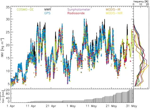
First of all, a multi-instrument intercomparison during the two months of High Definition Clouds and Precipitation for advancing Climate Prediction (HD(CP)2) Observational Prototype Experiment (HOPE) is performed to provide a realistic error estimate for the indi- vidual instruments observing IWV. The campaign took place from 1 April to 31 May 2013 at the Forschungszentrum Jülich (FZJ) in Germany (50.9°N, 6.4°E). During this two-month period, standard in- strumentation for observing water vapour at Jülich ObservatorY for Cloud Evolution (JOYCE), including Global Positioning System (GPS) antenna of the GeoForschungsZentrum Potsdam (GFZ), a scanning microwave radiometer (MWR), and a sunphotometer from Aerosol Robotic Network (AERONET), was complemented by frequent radio- soundings and four additional MWRs all within less than 4 km dis- tance of each other. In addition to the ground-based measurements, IWV estimates from two Moderate Resolution Imaging Spectrora- diometer (MODIS) retrievals, near infrared (NIR) and infrared (IR), that provide information with spatial resolution of 1 and 3 km, re- spectively, are available from satellite overpasses. The comparison re- veals a good agreement in terms of standard deviation (≤ 1 kg m−2) and correlation coefficient (≥ 0.98). The exception is MODIS, which appears to suffer from insufficient cloud filtering.
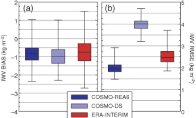
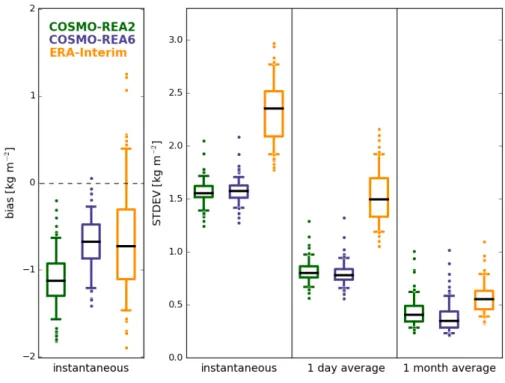
Based on the results of the intercomparison, observations of the Germany-wide GPS network are chosen for evaluation of two novel Consortium for Small-scale Modelling (COSMO) reanalyses — COSMO- REA2 and COSMO-REA6 — and ERA-Interim to assess their ability to represent IWV. The two highly resolved COSMO reanalyses ex- hibit a distinctly lower median standard deviation (1.6 kg m−2) than the global reanalysis ERA-Interim (2.4 kg m−2) over all GPS stations.
In this context it is also shown that a full reanalyses is superior to a dynamical downscaling which is computationally less costly.
For the assessment of the variability of IWV multiple methods are applied. The analysis of the auto-correlation of GPS observations
iii
and COSMO-REA6 simulation shows the importance of synoptic pro- cesses on meso-αscale and the analysis of the power spectrum shows a clear seasonal dependency of IWV variability. On meso-γ scales, standard deviations of IWV derived from MWR measurements re- veal high variability (>1 kg m−2) even at time scales of a few minutes.
This variability cannot be captured by measurements with lower tem- poral resolution. However, for time intervals above 30 min, observa- tions with 15 min resolution are as capable as MWR to capture the temporal variability. Spatio-temporal variability is assessed with the ICOsahedral Non-hydrostatic (ICON) simulation in Large Eddy Sim- ulation (LES) configuration with a resolution of 156 m for three days.
This study reveals that time differences of 30–45 min or a spatial mis- match of 9–10 km can induce standard deviations of approximately 0.7 kg m−2. This error depends on the weather situation.
The mean diurnal cycle of IWV is analysed in the COSMO reana- lyses, ERA-Interim, and GPS observations for spring and summer.
In general, the mean diurnal cycles exhibit a minimum in the morn- ing (4:00–10:00 UTC) and a maximum between 14:00 and 23:00 UTC.
While the amplitudes of the mean diurnal cycle of IWV observed with GPS vary between 0.4 and 2.0 kg m−2 (3.0–13.7%) in spring and 0.4–
2.6 kg m−2 (1.4–12.0%) in summer, the mean diurnal cycle simulated with the reanalyses exhibits smaller amplitudes and lower variabil- ity in their amplitudes. Also regional differences are found: coastal regions exhibit a shifted diurnal cycle with lower amplitudes while high altitudes exhibit larger amplitudes. Furthermore, the distinction between western and eastern weather situations shows that the strong advection of water vapour associated with western weather situations interferes with the evolution of the diurnal cycle.
The reanalysis COSMO-REA6 covering a time period of 19 years allows for assessing regional analysis of trends in IWV. Mean trends of 0.32 and 0.21 kg m−2per decade are analysed for COSMO-RE6 and ERA-Interim, respectively.
The present work characterizes IWV variability on meso scales over Germany and shows the importance of the consideration of IWV vari- ability e. g. for model evaluations and instrument intercomparisons.
iv
Z U S A M M E N FA S S U N G
Da Wasserdampf eine Schlüsselrolle in vielen atmosphärischen Pro- zessen auf unterschiedlichen Skalen, einschließlich Wolkenbildung und Niederschlag, spielt, ist er sowohl räumlich als auch zeitlich sehr variabel. Die Charakterisierung und Quantifizierung seiner Variabili- tät ist wesentlich für die Verbesserung von Parametrisierungen von Prozessen, die von Klima- und Wettervorhersagemodellen nicht auf- gelöst werden können, sowie für die Evaluierung von hoch auflösen- den Simulationen. In der vorliegende Arbeit liegt de Schwerpunkt auf der Charakterisierung und Quantifizierung der Variabilität von integriertem Wasserdampf (IWV) auf Skalen von Meso-αbis Meso-γ in Deutschland.
Zuallererst wird ein Messinstrumentenvergleich für den zweimo- natigen Zeitraum des High Definition Clouds and Precipitation for advancing Climate Prediction (HD(CP)2) Observational Prototype Ex- periments (HOPE) durchgeführt um eine realistische Fehlerabschät- zung für die einzelnen Instrumente zu geben. Die Kampagne fand vom 1. April bis zum 31. Mai 2013 am Forschungszentrum Jülich (FZJ) in Deutschland (50,9°N, 6,4°E) statt. Während dieser zwei Mo- nate wurde die standardmäßige Geräteausstattung des Jülich Obser- vatorY for Cloud Evolution (JOYCE), die eine Global Positioning Sys- tem (GPS) Antenne des GeoForschungsZentrums Potsdam, ein scan- nendes Mikrowellenradiometer (MWR) und ein Sonnenphotometer des Aerosol Robotic Network (AERONET) einschließt, ergänzt um regelmäßige Radiosondenaufstiege und vier weitere MWR, wobei al- le Geräte in einer Entfernung von weniger als 4 km zueinander po- sitioniert wurden. Zusätzlich zu den bodengebundenen Messungen, stehen IWV Abschätzungen von zwei Moderate Resolution Imaging Spectroradiometer (MODIS) Produkten, aus Messungen im infraro- ten und nahem infraroten Bereich, von Satellitenüberflügen zur Ver- fügung, die Information mit einer räumlichen Auflösung von jeweils 1 und 3 km liefern. Der Vergleich zeigt eine gute Übereinstimmung im Hinblick auf Standardabweichung (≤1 kg m−2) und Korrelations- koeffizienten (≥0, 98) mit Ausnahme von MODIS, das unter unzurei- chender Wolkenfilterung leidet.
Basierend auf den Ergebnissen des Vergleichs, werden Messungen des Deutschlandweiten GPS Netzwerks zur Evaluierung zweier neu- artiger COSMO Reanalysen — COSMO-REA2 und COSMO-REA6 — verwendet um ihre Darstellung des IWV zu bewerten. Die zwei hoch auflösenden COSMO Reanalysen weisen einen deutlich geringeren Median über alle GPS Stationen der Standardabweichung (1,6 kg m−2) auf als ERA-Interim (2,4 kg m−2). In diesem Zusammenhang wird
v
außerdem gezeigt, dass eine vollständige Reanalyse einem dynami- schen Downscaling, dass weniger rechenzeitintensiv ist, überlegen ist.
Für die Untersuchung der Variabilität von IWV werden mehre- re Methoden angewandt. Die Analyse der Autokorrelation von GPS Messungen und COSMO-REA6 Simulationen zeigt die Bedeutung synoptischer Prozesse auf der Meso-α-Skala. Die Analyse der Spek- traldichte zeigt eine deutliche jahreszeitliche Abhängigkeit der IWV Variabilität. Auf Meso-γ-Skalen zeigen die Standardabweichungen von IWV, gemessen mit einem MWR, sogar auf Zeitskalen von we- nigen Minuten eine hohe Variabilität (>1 kg m−2). Diese Variabilität kann von Messungen mit einer geringeren zeitlichen Auflösung nicht erfasst werden. Für Zeiträume über 30 min jedoch sind Messungen mit einer zeitlichen Auflösung von 15 min in der Lage die räumliche Variabilität genauso gut wiederzugeben, wie die Messungen mit ei- nem Mikrowellenradiometer. Die räumlich-zeitliche Variabilität wird aus einer Simulation mit dem ICOsahedral Non-hydrostatic (ICON) Modell in Large Eddy Simulations (LES) Konfiguration mit einer Auf- lösung von 156 m über drei Tage abgeschätzt. Diese Studie zeigt, dass Zeitunterschiede von 30–45 min oder eine räumlich Verschiebung von 9-10 km Standardabweichungen von ca. 0,7 kg m−2verursachen kann.
Dieser Fehler hängt von der jeweiligen Wettersituation ab.
Der mittlere Tagesgang des IWV im Frühling und Sommer wird in den COSMO Reanalysen, ERA-Interim und GPS Messungen un- tersucht. Grundsätzlich weist der mittlere Tagesgang ein Minimum am Morgen (4:00–10:00 UTC) und ein Maximum zwischen 14:00 und 23:00 UTC auf. Während die Amplituden des mittleren Tagesgangs des IWV gemessen mit GPS je nach Station zwischen 0,4 und 2,0 kg m−2 (3,0–13,7%) im Frühling und 0,4–2,6 kg m−2 (1,4–12,0%) im Sommer variieren, zeigt der mittlere Tagesgang der Reanalysen kleinere Am- plituden und eine geringer Variabilität in den Amplituden. Außer- dem werden regionale Unterschiede gefunden: küstennahe Regionen weisen eine Verschiebung im Tagesgang mit kleineren Amplituden auf während in höheren Lagen der Tagesgang größere Amplituden aufweist. Des Weiteren zeigt eine Unterscheidung zwischen westli- chen und östlichen Wettersituationen, dass die Wasserdampfadvekti- on, die mit westlichen Wetterlagen einhergeht, die Entwicklung des Tagesgangs überlagert.
Die Reanalyse COSMO-REA6 deckt einen Zeitraum von 19 Jah- ren ab und ermöglicht somit die regionale Analyse von Trends im IWV. Mittlere Trends von 0,32 und 0,21 kg m−2 pro Dekade werden in COSMO-REA6 und ERA-Interim gefunden.
Die vorliegende Arbeit charakterisiert die Meso-skalige Variabilität von IWV in Deutschland und zeigt die Bedeutung der Berücksichti- gung von IWV Variabilität z.B. für Modellevaluationen und Instru- mentenvergleiche.
vi
C O N T E N T S
a b s t r a c t iii
z u s a m m e n f a s s u n g v
i i n t r o d u c t i o n 1
1 i n t r o d u c t i o n 3
1.1 Motivation . . . 3
1.2 Objectives of the present study . . . 6
2 o b s e r vat i o n s 11 2.1 Global Positioning system . . . 11
2.1.1 General method . . . 13
2.1.2 Near-Realtime processing at GFZ . . . 15
2.1.3 Quality check for GPS measurements . . . 17
2.2 Microwave radiometer . . . 20
2.3 Radiosondes . . . 21
2.4 Sunphotometer . . . 22
2.5 MODIS . . . 23
3 m o d e l s 25 3.1 COSMO reanalyses . . . 25
3.2 ERA-Interim . . . 27
3.3 ICON . . . 27
ii r e s u lt s 29 4 m u lt i-i n s t r u m e n t c o m pa r i s o n 31 4.1 Matching the data . . . 33
4.2 Instrument intercomparison during HOPE . . . 34
4.3 Summary and conclusions . . . 37
5 i w v u n c e r ta i n t i e s i n m o d e l s i m u l at i o n s 39 5.1 Evaluation of reanalyses with GPS measurements . . . 39
5.1.1 Why a dynamical downscaling of COSMO is not good enough? . . . 39
5.1.2 Comparison of COSMO-REA2, COSMO-REA6 and ERA-Interim with GPS . . . 42
5.2 Evaluation of high resolution ICON with GPS meas- urements . . . 57
5.3 Summary and conclusions . . . 58
6 a s s e s s i n g t h e s m a l l-s c a l e va r i a b i l i t y 61 6.1 Auto-correlation function . . . 62
6.2 Scale analysis . . . 64
6.3 Variability in short time periods . . . 66
6.4 Spatio-temporal variability . . . 68
6.5 Summary and conclusions . . . 74
vii
viii c o n t e n t s
7 d i u r na l c y c l e 77
7.1 Harmonic analysis of diurnal cycle . . . 80 7.2 Seasonal dependency of diurnal cycle . . . 82 7.3 Dependency of diurnal cycle on geographic location . 91 7.4 Dependency of diurnal cycle on weather situation . . . 95 7.5 Relationship between diurnal cycle of IWV and diurnal
cycle of precipitation . . . 95 7.6 Summary and conclusions . . . 99
8 t r e n d s i n i w v 101
8.1 Decomposition of time series . . . 101 8.2 IWV trends . . . 103 iii s u m m a r y, c o n c l u s i o n s, a n d o u t l o o k 107 9 s u m m a r y, c o n c l u s i o n s, a n d o u t l o o k 109 9.1 Summary and conclusions . . . 109 9.2 Outlook . . . 112
iv a p p e n d i x 115
a g p s s tat i o n s 117
b t e m p o r a l a n d s pat i a l va r i a b i l i t y 121
c d i u r na l c y c l e o f c o s m o-r e a2 123
b i b l i o g r a p h y 125
A C R O N Y M S
AERONET Aerosol Robotic Network AIRS Atmospheric Infrared Sounder AMSL above mean sea level
CAM5 Community Atmosphere Model, version 5 CHAMP CHAllenging Minisatellite Payload
COSMO Consortium for Small-scale Modelling
COSMIC Constellation Observing System for Meteorology, Ionosphere, and Climate
CWT Circulation Weather Type DIAL Differential Absorption Lidar DWD Deutscher Wetterdienst
ECMWF European Centre for Medium-range Weather Forecasting
ERA-Interim European Centre for Medium-range Weather Forecasting (ECMWF) Re-Analysis Interim FZJ Forschungszentrum Jülich
GEWEX Global Energy and Water Cycle Exchanges project GFDL Geophysical Fluid Dynamics Laboratory
GFZ GeoForschungsZentrum Potsdam GLONASS GLObal NAvigation Satellite System GNSS Global Navigation Satellite System
GNSS-RO Global Navigation Satellite System-Radio Occultation GOME Global Ozone Monitoring Experiment
GPS Global Positioning System
GRACE Gravity Recovery And Climate Experiment G-VAP Global Energy and Water Cycle Exchanges
project (GEWEX) water vapor assessment HATPRO Humidity and Temperature Profiler
HD(CP)2 High Definition Clouds and Precipitation for advancing Climate Prediction
HErZ Hans-Ertel-Zentrum für Wetterforschung HOPE HD(CP)2Observational Prototype Experiment ICON ICOsahedral Non-hydrostatic
IGS International GNSS Service
IR infrared
IWV integrated water vapour
JOYCE Jülich ObservatorY for Cloud Evolution LEO Low Earth Orbiter
LES Large Eddy Simulation
ix
x a c r o n y m s
LHN latent heat nudging
LT local time
MERRA Modern ERA Retrospective Analysis for Research and Applications
MODIS Moderate Resolution Imaging Spectroradiometer MPI-M Max Planck Institute for Meteorology
MWR microwave radiometer
NAVSTAR Navigational Satellite Timing and Ranging
NIR near infrared
NWP numerical weather prediction
NRT near real-time
PPP Precise Point Positioning SAPOS Satellite Positioning
SCIAMACHY SCanning Imaging Absorption spectrometer for Atmospheric CHartographY
SSM/I Special Sensor Microwave Imager SYNOP surface synoptic observations WMO World Meteorological Organization ZHD Zenith Hydrostatic Delay
ZTD Zenith Total Delay
ZWD Zenith Wet Delay
Part I
I N T R O D U C T I O N
1
I N T R O D U C T I O N
1.1 m o t i vat i o n
Due to its influence on atmospheric processes on various scales, the importance of atmospheric water vapour cannot be underestimated.
It is not only the most effective greenhouse gas (Kiehl and Trenberth, 1997) but it plays also a key role in other major atmospheric processes including cloud formation and precipitation. It is also involved in surface and dynamic processes (cf. Fig. 1.1).
Water vapour has an important role in the water cycle (e. g. Bengts- son et al., 2014) as the atmospheric storage term with a residence time of only approximately nine days. Water of clouds, precipitation, soil, and water bodies, especially the ocean, vaporizes to water vapour.
Other sources of water vapour are the transpiration of vegetation and in the upper stratosphere methane oxidation. Water vapour is re- moved from the atmosphere by condensation especially during cloud formation and subsequent precipitation, which in turn increases the soil moisture, the run-off or is transported by rivers to the ocean. In Europe, most of the continental water emanates from the Atlantic and is also returned to the Atlantic. Due to the heterogeneous land sur- face in terms of vegetation and soil moisture, the water cycle is more complex over land than over ocean. Most of the described processes occur in the planetary boundary layer emphasizing its importance.
Condensation and vaporization are associated with the release or storage of latent heat. Therefore, transport of water vapour is always associated with energy transport. Water vapour transport occurs on different scales: from turbulent mixing in the boundary layer via con- vection to large-scale advection.
Water vapour interacts with radiation across the whole spectrum.
Its absorption properties in the infra-red spectrum make it the most important greenhouse gas. About 60% of the greenhouse effect can be attributed to water vapour (Kiehl and Trenberth, 1997). In com- bination with the dependency of saturation water vapour pressure on temperature, this results in a positive feedback due to warming.
Therefore, analysing trends in the amount of water vapour is import- ant.
Some of the processes involving water vapour as cumulus cloud formation and convection happen on such small scales that they can- not be resolved by numerical weather prediction (NWP) and climate models. These unresolved processes are nevertheless very important for accurate model simulations (Stevens and Bony, 2013). Especially
3
4 i n t r o d u c t i o n
Figure 1.1: The role of water vapour in atmospheric processes (adapted from Gérard et al. (2004)).
the interactions between convection and water vapour are not yet completely understood (Sherwood et al., 2010). Therefore, the under- standing of the water vapour distribution is crucial for improvement of the parametrization of these subgrid-scale processes.
The resolution of atmospheric models increased steadily. Thus, they become less prone to uncertainties induced by parametrizations at the cost of computationally expensive simulations. For example within High Definition Clouds and Precipitation for advancing Cli- mate Prediction (HD(CP)2), the first ever simulation with ICOsahed- ral Non-hydrostatic (ICON) in Large Eddy Simulation (LES) config- uration with a horizontal grid spacing of 156 m on the domain of Germany is run (Heinze et al., 2016). To evaluate these models, meas- urements resolving these small-scale processes are needed.
Operational measurements with a high temporal resolution of the profile of water vapour do not exist yet especially not within a dense network. Satellites observations could provide water vapour profiles though they are limited due to several reasons. When using obser- vations in the microwave band measurements are only available over ocean which is not suitable for the present work focusing on Germany.
Observations in the infrared band are limited to clear sky and they are not able to capture the lower troposphere which is, as mentioned above, crucial for the water cycle.
Measuring the total amount of water vapour within an atmospheric column is much easier. Considering the profile of water vapour it can be seen that at a typical midlatitude site about half of the total amount of water vapour is within the planetary boundary layer, meaning within about the lowest 1200 m, as the main sources are at the sur- face (Fig. 1.2). Furthermore, the variability of water vapour is highest
1.1 m o t i vat i o n 5
Figure 1.2: (left) solid line: Mean profile ofqvat station 2624 (50.9°N, 7.1°E) between Cologne and Bonn over the years 2007–2013 simulated with COSMO-REA6. shaded area: standard deviation of mean profile. (right) Water vapour integrated up to a distinct height level.
in the planetary boundary layer in absolute values. Although the ver- tical variability through vertical mixing and advection cannot be seen in the column integrated water vapour (IWV), the temporal and hori- zontal variability can be reproduced well from IWV measurements.
IWV is defined as the integral of the absolute humidityρv[kgm−3]
from the surface (z0) to the top of the atmosphere (zTOA):
IWV =
Z zTOA
z0
ρvdz. (1.1)
Its unit is 1 kg m−2. This is equivalent to 1 mm column of condensed water.
There is no unified naming convention for this variable. Frequently used names are e. g.: total column water vapour, precipitable water, or total-column precipitable water. In the present work the term in- tegrated water vapour (IWV) is used.
A wide range of techniques exists for measuring IWV. Different instruments sample different atmospheric conditions due to different integration times, beam widths, geometries, sampling strategies, loca- tions, etc. To asses which measurements can capture which variabilit- ies, a detailed intercomparison of a large set of instruments is needed.
Many studies compare various IWV measurements in different geo- graphical regions and for different time periods using different cri- teria for temporal and spatial matching and elevation corrections (cf.
6 i n t r o d u c t i o n
Bennouna et al., 2013; Martin et al., 2006; Morland et al., 2009; Pałm et al., 2010; Schneider et al., 2010; Torres et al., 2010). Frequently, these comparisons involve data sets with more than 1 h temporal and more than 20 km spatial difference as well as with different horizontal res- olutions. An assessment of the representativeness error is therefore needed. This holds true for relatively small temporal and spatial mismatches of e. g. ground-based instruments as well as for daily averages derived from observations of orbiting satellites which are provided only for one or two overpasses a day for the same location (Diedrich et al., 2016). The same is valid for radiosoundings, which are operationally conducted only once or twice a day at most loca- tions. To evaluate the representativeness of the latter measurements the variations during a day should be assessed. Furthermore, a better understanding of the diurnal cycle of IWV could improve the under- standing of the relationship between evaporation and precipitation since these processes determine primarily the amount of IWV.
1.2 o b j e c t i v e s o f t h e p r e s e n t s t u d y
This study aims at the quantification and characterization of IWV variability over a wide range of spatial and temporal scales — from meso-γ (2–20 km) to meso-α (200–2000 km) — over Germany focus- ing on terrestrial surfaces that are associated with strong variability.
To this end, the ability of models and instruments to capture this variability is assessed.
First of all there is the question how well state-of-the-art ground- based instruments can observe IWV variability. Therefore, a multi- instrument intercomparison during the two months of HD(CP)2 Ob- servational Prototype Experiment (HOPE) is performed to provide a realistic error estimate for the individual instruments observing IWV.
A wide range of instruments — Global Positioning System (GPS) an- tenna, scanning microwave radiometer (MWR), sunphotometer, fre- quent radiosoundings, infrared and near-infrared MODIS retrievals
— is compared. This unique set of observations is used for a stat- istical intercomparison to assess the representativeness of measure- ments from instruments with different temporal and spatial resolu- tion and which can measure under different atmospheric conditions.
Furthermore, the ability of the continuous measurements to capture variability within time intervals of a few minutes is assessed.
Secondly, the question arises whether IWV reanalysis can provide domain wide and temporal and spatially continuous IWV estimates that cannot be derived from instruments alone. Therefore, an evalu- ation of the models used in the present study with independent GPS observations is performed to assess how well IWV is represented in the respective model. In the course of this evaluation the question why a dynamical downscaling is not good enough and a full reana-
1.2 o b j e c t i v e s o f t h e p r e s e n t s t u d y 7
lysis is needed to assess IWV variability is tackled. The two novel Consortium for Small-scale Modelling (COSMO) reanalyses COSMO- REA2 and COSMO-REA6 performed within Hans-Ertel-Zentrum für Wetterforschung (HErZ) Simmer et al. (2015) are compared with the lower resolved reanalysis ECMWF Re-Analysis Interim (ERA-Interim).
To this end, the reanalyses are evaluated with GPS observations. The first ever Large Eddy Simulation (LES) with ICOsahedral Non-hydrostatic (ICON), which is run over Germany within the framework of HD(CP)2 is also evaluated with GPS. All models are used to assess IWV vari- ability. Therefore, the quality of the simulations has to be evaluated first.
Thirdly, this study aims at the quantification and qualification of IWV variability on meso scales. To this end, the evaluated observa- tions and simulations of IWV are used.
Previous studies assessing water vapour variabilities (e. g. Kahn et al., 2011; Fischer et al., 2012; Pressel et al., 2014) use scale analysis on scales of a few kilometres up to some hundreds of kilometres.
However, either these studies do not include the planetary boundary layer, where the absolute variability of water vapour is highest, or/
and they do not assess the meso-γ scale. Therefore, an extension of these analyses to smaller scales is needed. Additionally, the error of representativeness of measurements is assessed.
A further aim of the present work is to characterize the diurnal cycle of IWV, meaning the amplitude, as well as the time of minimum and maximum, focusing on the identification of regional differences and the influence of season and weather situations. Accompanied with a simultaneous analysis of the diurnal cycle of precipitation, a better understanding of the processes influencing the diurnal cycle of IWV can be given. These analyses are performed with GPS observa- tions as well as with reanalyses to assess the suitability of them for the analysis of the water cycle since reanalyses are frequently used for this purpose (e. g. Lorenz and Kunstmann, 2012).
Finally, since water vapour is the most important greenhouse gas and a warming of the atmosphere results in a strong positive feed- back, identification and estimation of the trend in IWV is import- ant. In the present study trends in IWV within a time period of up to 19 years (1995–2013) will be analysed in the COSMO reanalyses, ERA-Interim and GPS observations.
Summarized, the overarching question of the present work is:
How large is the variability of IWV on scales from meso-γ (2–20 km) to meso-α(200–2000 km) over Germany?
To assess this question the following scientific questions have to be tackled:
8 Bibliography
Q1 How well do IWV measurements of different instruments agree?
Q2 Which instrument allows to observe the variability of IWV on which scales?
Q3 To which degree can the COSMO reanalyses, ERA-Interim and ICON reproduce IWV and its variability and what is the benefit of high resolution simulations?
Q4 How variable is IWV on meso scales for time periods between a few minutes and a few days?
Q5 What are the characteristics of the diurnal cycle of IWV and how is it influenced by region, season and weather situation?
Q6 Is there a trend in IWV and how does it differ across Germany?
The present study is structured as follows. Chap. 2 and Chap. 3 provide information about all observations and model simulations which are used to assess the variability of IWV. In Chap. 4, a multi- instrument comparison is given. Chapt. 5 provides an extended eval- uation of the three reanalyses COSMO-REA2, COSMO-REA6, and ERA-Interim, and also compares a dynamical downscaling with a full reanalysis. Additionally, ICON in LES configuration is evaluated with GPS observations. The following chapters contain the actual as- sessment of IWV variabilities. Firstly, in Chap. 6 variability on meso-γ scale and below are assessed with various observations and a highly resolved ICON simulation. Secondly, in Chap. 7 the diurnal cycle of IWV is characterized with reanalyses and GPS observations focus- ing on the influence of season, region and weather situation. This chapter is complemented by a simultaneous analysis of the diurnal cycle of IWV and precipitation. Thirdly, in Chap. 8 a trend analysis of IWV within reanalyses and GPS observations is performed. Fi- nally, in Chap. 9, the presented results are summarized. Additionally, suggestions for future research are presented.
The multi-instrument comparison as presented in Sect. 4 and the study on temporal IWV variability presented in Sect. 6.3 have recently been published in
Steinke, S., Eikenberg, S., Löhnert, U., Dick, G., Klocke, D., Di Gir- olamo, P., and Crewell, S. (2015). Assessment of small-scale integ- rated water vapour variability during HOPE.Atmospheric Chemistry and Physics, 15(5):2675–2692.
The evaluation of a dynamical downscaling of ERA-Interim, COSMO- REA6 and ERA-Interim with GPS observations as presented in Sect. 5.1.1 has recently been published in
Bibliography 9
Bollmeyer, C., Keller, J. D., Ohlwein, C., Wahl, S., Crewell, S., Friederichs, P., Hense, A., Keune, J., Kneifel, S., Pscheidt, I., Redl, S., and Steinke, S. (2015). Towards a high-resolution regional reana- lysis for the European CORDEX domain. Quarterly Journal of the Royal Meteorological Society, 141(686):1–15.
2
O B S E R VAT I O N S
In order to address the variability of IWV on different spatio-temporal scales and to evaluate various models (Sect. 3), a wide range of instru- ments — GPS (Sect. 2.1), microwave radiometer (Sect. 2.2), sunphoto- meter (Sect. 2.4), MODIS (Sect. 2.5), and radiosondes (Sect. 2.3) — is used in this study. The measurement principles of the instruments as well as their error characteristics and limitations are described in the following (Tab. 2.1. An extensive comparison of the instruments for a case study is provided in Sect. 4.
2.1 g l o b a l p o s i t i o n i n g s y s t e m
The principle of deriving IWV from the signal of Global Navigation Satellite System (GNSS) satellites is based on the fact that the signal transmitted from a satellite is refracted by the atmosphere. This leads to an increase of the path length through the atmosphere (Bevis et al., 1992) because the refraction depends, amongst other things, on the amount of water vapour in the atmosphere.
The two globally operational systems are the US-American Navig- ational Satellite Timing and Ranging (NAVSTAR) - Global Position- ing System (GPS) and the Russian GLObal NAvigation Satellite Sys- tem (GLONASS) nowadays. The European Galileo and the Chinese
BeiDou are currently being developed into operational systems. The Beidou is Chinese for the Big Dipper, which includes the north star that was used for navigation.
four systems differ in number and orbit constellation of their satellites as well as in the frequencies of the emitted signal. Once, all four sys- tems are fully deployed, approximately 120 navigation satellites will be available. Therefore, the combination of GNSS will significantly in- crease the number of observed satellites and consequently optimize the spatial geometry and improve continuity and reliability of posi- tioning. Nowadays, there are several studies combining two systems, especially GPS with GLONASS or BeiDou (e. g. Cai and Gao, 2013) and also combinations of all four systems (Li et al., 2015).
In general, there are two measurement geometries. Firstly, the sig- nal emitted by a GNSS satellite and refracted by the atmosphere is received by a Low Earth Orbiter (LEO), e. g. the German CHAllen- ging Minisatellite Payload (CHAMP) satellite, the US/German Grav- ity Recovery And Climate Experiment (GRACE)-A satellite or the six satellites of the Taiwan/US FORMOSAT-3/Constellation Observing System for Meteorology, Ionosphere, and Climate (COSMIC) mission (Wickert et al., 2009). Then with the so called Global Navigation Satel- lite System-Radio Occultation (GNSS-RO) method, vertical profiles of
11
12 o b s e r vat i o n s
Table2.1:Temporalresolution,spatialresolutionorrepresentativeness,limitations,systematic(s),random(r)orcombinederrorofmeasurementsasfoundinliteraturefortheinstrumentsusedinthepresentstudy(fromSteinkeetal.(2015)).
instrumenttemporalspatiallimitationsuncertaintyreferenceresolutionresolution/kgm −2or%representativeness
MWRHATPRO≈2s3.5°beamwidth;nomeasurements0.5(s)Roseetal.(2005)122mbeamwidthduringrain0.5-0.8(r)at2kmheight
GPS15minca.32km anozenithmeasurement1-2Gendtetal.(2004)
sunphotometer10min1.2°beamwidthdaytime/clear-skyonly,10%Alexandrovetal.(2009)directiontowardssun
GrawDFM-09atleast1hdriftupto100kmdrift,measurement1.2(s)WangandZhang(2008)radiosondetakesca.1h1.7(r)
MODIS-NIR≤6timesperday1kmdaytime/clear-skyonly5-10%GaoandKaufman(2003)
MODIS-IR≤6timesperday3kmclear-skyonly5-10%Seemannetal.(2003)
aTheplanetaryboundarylayerwithanassumedheightof2kmcontributesmosttoIWV.TheGPSslantswiththelowestangles(7°)leavetheboundarylayerinadistanceofapproximately16kmfromtheGPSstationandtheslantsareonaverageazimuthally,equallydistributed.Thisleadstoaspatialrepresentativenessof32km.
2.1 g l o b a l p o s i t i o n i n g s y s t e m 13
atmospheric parameters — temperature and water vapour — starting in the upper boundary layer can be derived globally. Secondly, the signal is received by a receiver on the ground. This geometry allows for deriving integrated parameters as IWV. The latter method is used in this study.
In the following, the general method of GPS is explained and after- wards the configurations used by GFZ for near real-time processing is described. An explanation of the quality checks applied to the data set provided by GeoForschungsZentrum Potsdam (GFZ) follows.
2.1.1 General method
The GPS system comprises of two parts: the satellites on the one hand and the network of ground-based stations, consisting of antenna and receiver, on the other hand. 24 GPS satellites are in an orbit at approximately 20 200 km height. They transmit signals with carrier waves with frequencies of 1575.42 MHz (L1) and 1227.60 MHz (L2).
These carrier waves are amplitude-modulated with information on position and time of their respective atomic clock.
Since little shifts in the position of the antenna can lead to differ- ences in the derived IWV, the antenna needs to be firmly fixed on ground. The ground-based GPS stations can receive at 12 different channels. That means that such a receiver can detect the signal of up to 12 satellites simultaneously. For the measurements to be scien- tifically usable, the following criteria need to be fulfilled: Firstly, the signals of at least four satellites need to be received. Secondly, only signals that reach the receiver at an elevation angle higher than 7°
are used. This optimum cut-off angle depends on the application. A low cut-off angle implies a good geometry and a low uncertainty in the individual IWV estimates (Ning and Elgered, 2012). However, if the angle is too low, systematic errors are introduced, for example in- terference by signal multi-path, including scattering (Elósegui et al., 1995). Additionally, the signal is too weak if the path through the atmosphere is too long and the atmosphere is not homogeneous.
In the following, the method to derive the position of the receiver as described, e. g. by Seeber (2008) is summarized. The position of the receiver can be determined by using the pseudo rangePR. This is the product of the speed of lightcand the time the signal takes from the satellite to the ground-based receiver, i. e. the time difference of the two clocks. It can be determined with an accuracy of a few meters:
PR= c(t−T) =R+c(dt−dT) +dion+dtro+e (2.1) with satellite clock errordt and receiver clock errordT. Ris the slant range between the satellite and receiver, dion anddtro are the delays
14 o b s e r vat i o n s
due to ionospheric and tropospheric components, respectively, and e is the the observation noise.
In contrast to the accuracy of a few meters achieved by using PR, the tropospheric delay is in the mm-scale. In order to achieve this high accuracy, the phase difference between the carrier phase of the satellite signal φsat and the reference phase of the receiver φrec is ad- ditionally used:
Φ=λ(φsat−φrec) = R+c(dt−dT) +λN+dion+dtro+e (2.2) where λ is the wavelength of the carrier wave and N is its integer phase ambiguity. Because of the dispersive nature of the ionosphere, the ionospheric delay can be approximated by combining the meas- urements of the two frequencies L1 and L2. To eliminate all the unknowns, equations for different time steps and different satellite receiver combinations are set up. This over-determined equation sys- tem can be solved e. g. with least square adjustment.
In principle, two approaches exist to derive the tropospheric delay.
With the network approach, the tropospheric delay for all receivers within a network is computed simultaneously which leads to a huge computational cost for large networks of a few hundred stations. In- stead, the Precise Point Positioning (PPP) is used (Zumberge et al., 1997). This method exhibits an accuracy comparable to the network approach (Stoew et al., 2001) but is much faster for large networks.
First, the orbits of the satellites and their clock corrections are de- termined from a globally distributed network of a few GPS receivers.
These parameters are fixed values for each satellite. The following steps are conducted for each station individually.
To derive IWV from the tropospheric delay dtro, the dry tropo- spheric component is subtracted and the wet delay is mapped to zenith. The Zenith Total Delay (ZTD) is defined as the sum of the Zenith Hydrostatic Delay (ZHD) and the Zenith Wet Delay (ZWD):
ZTD= ZHD+ZWD (2.3)
To build up a relation with dtro, the mapping functions mh(β) and mw(β) for the hydrostatic delay and the wet delay, respectively, are needed. They depend on the elevation angle βat which the ground station receives the signal of the satellite:
dtro =mh(β)ZHD+mw(β)ZWD (2.4) In general, a mapping function is a continued fraction of sin1(
β) with several parameters, which can be some combination of constants and functions of geographic location, local meteorological conditions, and season (Younes and Elmezayen, 2012).
2.1 g l o b a l p o s i t i o n i n g s y s t e m 15
ZHD is approximated by surface pressureps, latitudel, and height hof the receiver, with a high accuracy (Saastamoinen, 1972):
ZHD=10−6k1Rd Z
z
ρdz≈k01ps (2.5)
with the specific gas constant for dry airRd =287.05 Jkg−1K−1, air density ρ, empirical constant k1, which is evaluated by actual meas- urements of the refractive index (Thayer, 1974), and the constant k01 depending onk1, height, and latitude of the receiver. The Zenith Wet Delay (ZWD) depends on a function of the weighted mean temperat- urek0(Tm)and the integral of water vapour densityρw :
ZWD=k0(Tm)
Z
zρwdz. (2.6)
The weighted mean temperature can be approximated by a function of the surface temperature Ts, which introduces an error of approx- imately 2% (Bevis et al., 1992). The surface temperature Ts is used because it can be measured at the GPS station itself or interpolated from the next surface synoptic observations (SYNOP) stations. How- ever, since the diurnal variation of the surface temperature is larger than the diurnal variation of the mean temperature of the atmosphere, this approximation can lead to an error of less than 0.1 kg m−2 in the amplitude of the diurnal cycle and a shift of the diurnal cycle by 1 to 2 hours later (Morland et al., 2009).
With equations 2.3 and 2.5, IWV can be written as:
IWV =
Z
zρwdz= 1
k(Ts)(ZTD−ZHD) (2.7) With this technique, IWV can be derived with an accuracy of 1–
2 kg m−2 (Gendt et al., 2004), which is an absolute uncertainty. This means it does not depend on the magnitude of IWV.
2.1.2 Near-Realtime processing at GFZ
The network of ground-based stations, GFZ makes use of the Satellite Positioning (SAPOS) network operated by the land surveying offices of the federal states (Landesversmessungsämter) and additional own GPS stations. Nearly 300 GPS stations in Germany and some stations abroad are used to derive IWV. The receivers produce rawfiles with a temporal resolution of 30 s.
GFZ uses EPOS software (Gendt et al., 2004) for near real-time (NRT) data processing. This software uses the least squares adjust- ment. At the beginning of each day the positions of the GPS sta- tions are determined using International GNSS Service (IGS) final products. These positions are fixed for one day. The initial values
16 o b s e r vat i o n s
for the processing are 3-hourly ultra rapid orbit predictions, which are performed with global hourly IGS data within a sliding 24 h data window. These orbit predictions are used as basis for both orbit and clock adjustment. Higher accuracy of these adjustments is achieved by orbit estimation with data of 20 well-distributed global sites and five additional German stations in a 12 h window.
The next step of data processing uses the precise point positioning which allows parallel computing of several sites in clusters keeping computing time low even for several hundred stations and a high temporal resolution of 15 minutes. Within this step, a system of 40–
50 equations, depending on the number of satellites visible to the re- ceiver within the time interval of 15 minutes, is solved with the least squares adjustment to retrieve ZTD for each station. The standard deviation of ZTD (σZTD) is computed from the inversion of the nor- mal equations and scaled with the standard deviation of unit weight computed from the least square residuals (Gendt et al., 2004).
The mapping functions for the dry and wet delay are both con- tinued fractions from Niell (1996) whose coefficients depend on the latitude of the site. Additionally, the coefficients of the mapping func- tion of the dry delay depends on the height above sea level of the ob- serving site and on the day of the year. Surface pressure and surface temperature needed to derive IWV from ZTD are either measured dir- ectly at the GPS station or interpolated from the smallest surrounding triangle of SYNOP stations, which is the case for most GPS stations.
A height correction is applied beforehand and stations with a height above 1000 m AMSL are excluded. The RMSE due to the correction of pressure is normally 0.3 hPa and can reach 0.5−1 hPa, which cor- responds to 0.2 to 0.4 kg m−2 (Gendt et al., 2004).
The near-realtime processed GPS measurements exhibit two dis- tinct features: firstly, they show a jump at the beginning of most full hours, which can be up to 1 kg m−2. These jumps are caused because each complete hour is processed at the same time and the retrieval tend to smooth these four quaterhourly measurements. Secondly, even larger differences can be seen between the observations at 23:45 UTC and 00:00 UTC of the next day. This is a known characteristic of the near-real-time processing of GPS data, which is also seen in the investigation of the daily cycle at stations in North America by Dai et al. (2002). The exact reason for this feature is not finally clarified yet and subject of ongoing investigation. However, the measurements of the beginning of the day which exhibit such large differences to the last measurements of the day before also exhibits largeσIWV and can be filtered with the quality check described in Sect.. 2.1.3.2.
2.1 g l o b a l p o s i t i o n i n g s y s t e m 17
Figure 2.1: Number of GPS stations whose measurement period covers at least a distinct percentage of the time period 2007-2013.
2.1.3 Quality check for GPS measurements
GFZ provides a data set with measurements at about 400 GPS stations whereof 294 are located within the domain of COSMO-REA2 with a height difference lower than 200 m to the next reanalysis grid point (cf. Sect. 3.1) as of 1 January 2014. Before GPS measurements are used for any further investigations, a quality check is performed. First, stations with data available for too short time periods and erroneous stations are removed (cf. Sect. 2.1.3.1). Afterwards, single measure- ments are removed through a plausibility check and a threshold of σIWV is computed during the processing of IWV (cf. Sect. 2.1.3.2).
2.1.3.1 Quality check of stations
Visual inspection and different test algorithm have been developed to identify and subsequently remove erroneous stations. Some stations, mainly non-German stations, in general show unrealistic values or behaviour of IWV. The IWV measurements at the station in Brussels, Belgium (BRUS) for example are distinctly lower than close by radio- soundings. This is due to the too low surface pressure used for the processing of the data. Four stations show such biases due to wrong surface pressure. Three stations inhibit regular jumps in the mean diurnal cycle probably due to different data sources of surface pres- sure used at different times (Fig. 2.2). Furthermore, 19 stations show sudden jumps when differences with a nearby station or model data are analysed. This might occur due to a change of receiver or antenna but cannot be clearly attributed in retrospect. Another five stations show regular patterns in the time series of differences to a nearby sta-
18 o b s e r vat i o n s
Figure 2.2: Mean diurnal cycle of IWV derived from GPS measurements for the years 2009-2013 at station 0291 in the vicinity of Salzburg (47.8°N, 12.9°E).
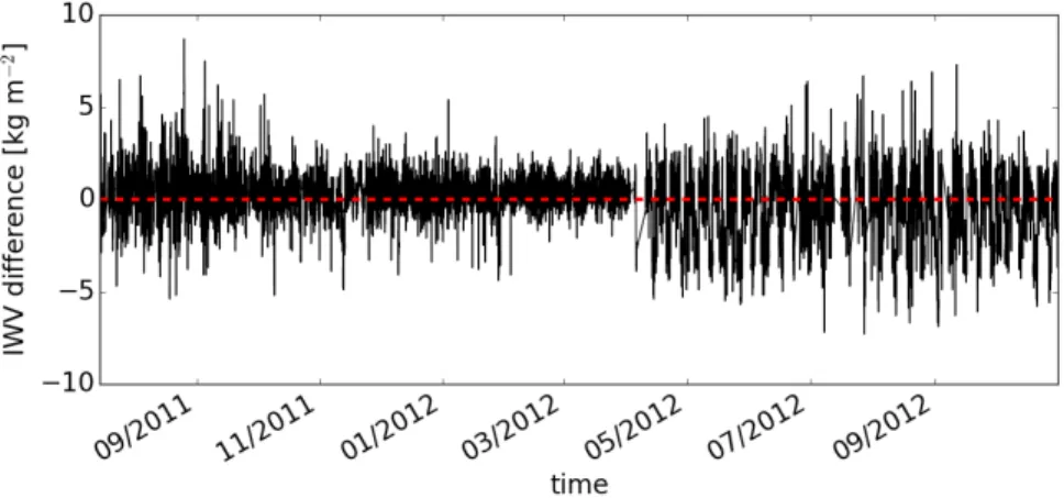
Figure 2.3: Time series of differences between IWV of GPS station 2577 (51.2°N, 6.8°E) and IWV of GPS station 2579 (51.3°N, 6.4°E).
tion for some times (cf. Fig. 2.3) and are rejected. The reason for these patterns is still under investigation. A detailed list of stations with the respective reasons of rejection can be found in Appendix A.
After the quality checks of the stations, 183 of 294 stations (64%) within the domain of COSMO-REA2 remain to be used for further analysis.
2.1.3.2 Quality check of single of measurements
Two checks are applied to the measurements: a plausibility check and a check of σIWV. In general, only IWV measurements higher than 1 kg m−2 and lower than 50 kg m−2 are considered, since meas- urements outside this range are not considered to be meteorological
2.1 g l o b a l p o s i t i o n i n g s y s t e m 19
Figure 2.4: Standard deviation (top) of GPS measurements compared to mi- crowave radiometer measurements and reduction of the number of measurements (bottom) if GPS data withσIWV higher than a distinct threshold is rejected. Measurements were carried out in April and May 2013 at JOYCE.
consistent within the investigated domain of central Europe. Less than 1% of the measurements are removed due to this criterion.
As described in Chapter 2.1.2, while processing ZTD,σZTD is com- puted which provides information on the accuracy of the delay. A rough estimate in terms of IWV isσIWV = 0.15 *σZTD. To test which threshold ofσIWV is useful, a two month time series (April and May 2013) of GPS and simultaneous microwave radiometer measurements in Jülich is used. A previous study (Steinke et al., 2015) shows good agreement between measurements of both instruments except for very few samples especially during the first hour of the day, which is a known issue of the GPS near real-time retrieval (cf. Sect. 2.1.2). A fil- tering depending on different thresholds of σIWV shows a reduction in standard deviation between microwave radiometer and GPS meas- urements with lower thresholds for σIWV. It has to be mentioned that this quality check is not applied to the GPS measurements of the multi-instrument comparison (Sect. 4) since the development of this check is partly based on this study.
The thresholdσIWVTHRis determined to be 0.85 kg m−2due to the following considerations. With this threshold the standard deviation is reduced from 0.89 kg m−2 to 0.84 kg m−2 (Fig. 2.4). Especially the GPS measurements with high differences up to 4 kg m−2compared to the microwave radiometer measurements are filtered out. Meanwhile, the reduction of the number of measurements is less than 1%. Lower thresholds do not distinctly reduce the standard deviation but reduce the number of measurements significantly. Therefore, the threshold σIWVTHR =0.85 kg m−2is used for the whole data set.
20 o b s e r vat i o n s
2.2 m i c r o wav e r a d i o m e t e r
Microwave radiation is defined as radiation with frequencies between 3 and 300 GHz. A passive microwave radiometer (MWR) measures this radiation emitted by the atmosphere, i. e. gases and hydromet- eors, at selected frequencies in this range. The range of frequencies (20–60 GHz is suited for deriving liquid water path, IWV, as well as temperature and humidity profiles. This is enabled through the dis- tinct absorption characteristics of water vapour and oxygen within this frequency range, meaning an absorption line of water vapour at 22.235 GHz and an absorption band of oxygen at 60 GHz. The emis- sion of both gases can be measured with a MWR. Furthermore, the emission of atmospheric liquid water increases with frequency. Typ- ically, these measurements are calibrated directly to so-called bright- ness temperatures. For this purpose, the Rayleigh-Jeans approxima- tion is normally used for microwave radiation. This approximation assumes a linear relation between spectral radiance and temperat- ure. For very low temperatures occurring at frequencies lower than 40 GHz, this relationship no longer holds true and errors of some tenth degrees can occur (Janssen, 1993). Due to this, the relation between brightness temperature and spectral radiance is better de- scribed with Planck’s function:
Bν(T) = 2hν
3
c2
1
ehν/kBT−1. (2.8)
Here T is the temperature of a black body, which emits the spectral radiance Bat frequency ν,his the Planck’s constant,cis the speed of light, andkB is the Boltzmann’s constant.
In principle, a MWR consists of an antenna, several amplifiers, and a detection system. The MWR Humidity and Temperature Pro- filer (HATPRO) manufactured by Radiometer Physics GmbH1 has an antenna with a half power beam width of 3.5° for the water vapour sensitive channels. Thus, the MWR measures a comparatively nar- row part of the atmosphere. The incident radiation is spilt with a wire grid in both orthogonal polarizations. This allows simultaneous processing by two receivers after amplification. One receiving unit measures at seven frequencies between 51.3 and 58.0 GHz along slope of the oxygen absorption complex, while the other unit receives the radiation at seven frequencies along the water vapour absorption line (22.24 GHz, 23.04 GHz, 23.84 GHz, 25.44 GHz, 26.24 GHz, 27.84 GHz) and one frequency in an atmospheric window (31.40 GHz). From the brightness temperatures of the latter seven frequencies, the IWV, the integrated liquid water content and a vertically coarse resolved water vapour profile with up to three independent layers (Löhnert et al., 2009) can be derived. With a low noise level of approximately 0.05 K
1 http://www.radiometer-physics.de
2.3 r a d i o s o n d e s 21
in the measured brightness temperatures, HATPRO is able to detect small variations in atmospheric water vapour.
IWV is derived following a statistical approach based on a least squares linear regression model (Löhnert and Crewell, 2003) from the multi-frequency brightness temperatures TB assuming the error characteristics mentioned above. Its general form can be written as
IWV = c0+c1·TB+c2·TB2. (2.9) To derive the coefficientsc0,c1, andc2, a training data set is used. This data set consists of more than 13 000 non-precipitating radiosound- ings at De Bilt, Netherlands, which is about 150 km apart from JOYCE.
With this algorithm, IWV can be derived with a random error of approximately 0.5–0.8 kg m−2from zenith measurements (Maschwitz et al., 2013). The systematic error is assumed to be 0.5 kg m−2 and the noise level is 0.05 kg m−2. Note that the MWR is able to measure automatically with a temporal resolution of ca. 2 s under all weather conditions with the exception of when the radome is wet. In these cases, no IWV values are provided based on visual inspection.
2.3 r a d i o s o n d e s
Attached to a balloon, instruments can ascent through the atmosphere.
In combination with a GPS sensor, which determines the position of the sonde, the instruments measure profiles of pressure, temperature and humidity. Additionally, profiles of wind speed and wind direc- tion are derived from the movement of the sonde.
The radiosoundings used in this study are performed with Graw DFM-09 sondes2. These feature a thin film capacitance sensor in order to measure relative humidity. Together with the temperature meas- urements and the pressure profile derived from GPS measurements, the absolute humidity is computed. Afterwards, the absolute humid- ity is integrated to derive IWV from the radiosoundings.
Several studies asses the error of radiosonde measurements show- ing that the error strongly depends on the type of radiosonde. Fur- thermore, the systematic and random error of the relative humidity sensor depend on temperature and differ between day- and nighttime.
A World Meteorological Organization (WMO) comparison (Nash et al., 2011) to IWV derived from GPS showed that the difference between Graw DFM-09 and GPS is 2 kg m−2 higher during daytime than dur- ing nighttime. Other radiosonde types showed the opposite beha- viour. The reason for this could be that the correction algorithm ap- plied by the Graw software probably overcorrects the original dry bias. It is not known if the correction of the software was changed since the test. In general, IWV comparisons of radiosondes with ca-
2 http://www.graw.de
22 o b s e r vat i o n s
pacitance sensors to GPS measurements show a dry bias for the ra- diosondes of approximately 1.2 kg m−2 during daytime due to sensor exposition to solar radiation (Wang and Zhang, 2008).
An additional error source is the drift of radiosondes during as- cent. The radiosondes used in this study drift horizontally on aver- age 5 km during their ascent to 850 hPa and 39 km to the 200 hPa-layer.
The maximum drifts to these pressure levels are 8 km and 106 km, re- spectively. Therefore, it has to be kept in mind that a radiosonde may well sample a different air mass than a zenith-pointing ground- based instrument would do. However, IWV variability is low above the boundary layer because the flow is determined by large-scale ad- vection and therefore homogeneity is high (Shao et al., 2013).
2.4 s u n p h o t o m e t e r
The sunphotometer (CE 318 N-EBS9, Cimel Eletronique S.A.S3) used in this study measures the extinction of direct solar irradiance and sky radiance at 9 wavelengths (340 , 380 , 440 , 500 , 675 , 870 , 937 , 1020 , and 1640 nm) fully automatically. Allowing for the extinction due to aerosols, the extinction due to the amount of water vapour in the line of sight to the sun Tw can be derived from the extinction at 937 nm. The extinction can be described with the following equation
Tw=exp[−a(m·IWV)b] (2.10)
where a, and b are constants, and m is the relative optical air mass (Schmid et al., 2001). From this relationship, IWV can be derived with an accuracy of 10% (Alexandrov et al., 2009).
The sunphotometer is part of Aerosol Robotic Network (AERONET), meaning that data processing is performed by the National Aeronaut- ics and Space Administration (NASA) (Dubovik et al., 2006). The data used within the present study is of quality level 1.0 and has a tem- poral resolution of approximately 10 min.
Since the sunphotometer measures the direct sunlight, its IWV re- trieval is limited to daytime and clear-sky conditions. Additionally, since the instrument tracks the sun, the retrieved IWV is not zenith viewing, but along a slant path through the atmosphere. This implies that it samples a different atmospheric volume than zenith-pointing instruments. An additional problem due to the changing viewing paths can occur when the sunphotometer is measuring at low solar zenith angles in combination with high IWV values. This saturation could lead to transmission approaching zero (Ingold et al., 2000).
3 http://www.cimel.fr
2.5 m o d i s 23
2.5 m o d i s
The Moderate Resolution Imaging Spectroradiometer (MODIS) is a space-borne, passive, whisk-broom scanning radiometer which meas- ures the radiation backscattered and emitted from Earth, clouds, and atmosphere at 36 spectral bands between 0.4 and 14.4 µm wavelength.
Two MODIS instruments are currently operational in space on board of NASA’s sun-synchronous near-polar-orbiting Earth Observing Sys- tem (EOS) Terra and Aqua platforms4. This enables a full global coverage every one to two days. With an orbit height of approxim- ately 705 km and a scanning pattern of ±55◦, the swath dimension of MODIS amounts to 2330 km across-track and 10 km along-track (at nadir).
Two standard IWV products exist for MODIS: the infrared retrieval (MODIS-IR) and the near-infrared retrieval (MODIS-NIR). Within the present study, MODIS Level 2 MODIS-IR and MODIS-NIR products from Collection 5.1 are used, which have a grid resolution of 3 and 1 km, respectively5.
MODIS-NIR utilizes three channels located within the water va- pour absorption wavelengths, namely 0.905 µm, 0.936 µm and 0.94 µm, and two non-absorbing channels, namely 0.865 µm and 1.24 µm. The ratios in reflected NIR radiation from water vapour absorption chan- nels to window channels give the atmospheric water vapour trans- mittances. From these, IWV is obtained from look-up tables based on line-by-line calculations. Note that single and multiple scattering effects are assumed to be negligible. The estimated errors in retrieved IWV are typically 5–10% and are mostly assigned to uncertainties in the spectral reflectance of the surface targets and in uncertainties in the amount of haze over dark surfaces. For details on the MODIS-NIR retrieval see Gao and Kaufman (2003).
MODIS-IR utilizes two water vapour absorption bands which de- liver information on the moisture distribution and three window bands which also have weak water vapour absorption. From the radiances measured at these bands, water vapour profiles are retrieved via a statistical regression algorithm based on previously determined re- lationships between radiances and water vapour profiles. Though computationally efficient, this algorithm is sometimes non-physical.
Therefore, a non-linear iterative physical algorithm is applied to the retrieved profiles, aiming to improve the solution, that is reduce the known overestimation of IWV. For details on the MODIS-IR retrieval see Seemann et al. (2003).
Being based on thermal radiation, MODIS-IR is available for both day- and nighttime over ocean and land. However, it is limited to clear-sky situations. The same goes for MODIS-NIR, which is ad-
4 http://modis.gsfc.nasa.gov/
5 http://modis.gsfc.nasa.gov/data/
24 o b s e r vat i o n s
ditionally restricted to daytime and highly reflective surfaces that means land and no ocean. Both MODIS retrievals, if applied to over- cast scenes, miss information from within and below clouds.
3
M O D E L S
Additionally to the observations, runs of different models are used to address the spatio-temporal variability of IWV. Reanalyses, as the COSMO reanalyses (cf. Chap. 3.1) and ERA-Interim (cf. Chap. 3.2), merge observations and modelling for best estimates of atmospheric state over a time period of several years. Hence, a reanalysis is neither pure observation nor pure model. However, to distinguish it from pure observations we use the notation model as it provides gridded, three dimensional, temporally continuous information. The advantages of a reanalyses in comparison to an operational model are first the usage of one model version for a longer time period and therefore no inconsistency in the simulation due to a change in the model version, and second observations which become available too late for operational usage can be assimilated. The novel model ICON (cf. Chap. 3.3), which is run in a LES configuration (Heinze et al., 2016) provides a highly resolved simulation over Germany. In the follow- ing, a description of these models and their specific output is given.
3.1 c o s m o r e a na ly s e s
Within the Hans-Ertel-Zentrum für Wetterforschung (HErZ; Weiss- mann et al. 2014, Simmer et al. 2015), two regional reanalyses are produced: COSMO-REA6 (Bollmeyer et al., 2015) and COSMO-REA2 (Wahl et al., 2016), with a resolution of ca. 6 km and 2 km, respectively.
In the following, the Consortium for Small-scale Modelling (COSMO) and the special reanalyses framework is introduced.
The limited-area, numerical weather prediction (NWP) model COSMO1 is a non-hydrostatic, fully compressible model of the atmosphere. The thermo-hydrodynamical equations describing compressible flow in a moist atmosphere are solved using a finite-difference method on an Arakawa-C grid (Arakawa and Lamb, 1977). As for the coordin- ates, the model uses rotated latitude/longitude coordinates in the horizontal and time-independent terrain-following coordinates in the vertical. COSMO uses a bulk-water continuity model for the grid- scale precipitation (Doms et al., 2011) and a Tiedtke mass flux scheme for subgrid-scale convection (Tiedtke, 1989). The radiative transfer scheme used in COSMO is described in Ritter and Geleyn (1992).
Both reanalyses, COSMO-REA6 and COSMO-REA2, are simulated with COSMO. The domain of COSMO-REA6 is the CORDEX-EURO-
1 http://www.cosmo-model.org/
25
26 m o d e l s
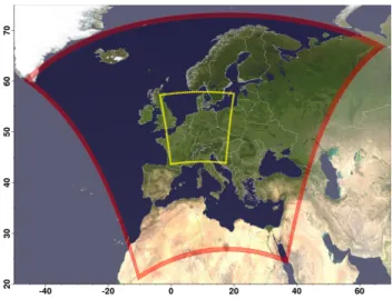
Figure 3.1: Domain of COSMO-REA6 (red) and COSMO-REA2 (yellow).
(Source: Bollmeyer et al. (2015))
11 domain, which covers Europe (Fig. 3.1). However, the used grid is finer than the original CORDEX-EURO-11 grid, i. e. 40 vertical layers and a horizontal grid spacing of 0.055°, which corresponds to approx- imately 6.2 km. The time step of the model is 50 s. The setup of the reanalysis, which uses COSMO version 4.25 (28 September 2012), is generally the same as the setup of COSMO-EU (Steppeler et al., 2003), which was run operationally by DWD until 30 November 2016. The initial field is provided at 00:00 UTC at the start date. From this field, a 6 hours run with a full data assimilation is initiated. After six hours, a snow analysis is performed and a new 6 hours run is started. This lasts until the end of the day. Then a sea surface temperature ana- lysis is performed, followed by a snow analysis and a soil moisture analysis. Then the next day is started and so on until the end of the simulation period is accomplished. The initial field and boundary conditions originate from ERA-Interim (Chap. 3.2).
The COSMO-REA6 run provides initial fields and boundary con- ditions for COSMO-REA2, which has a finer resolution, i. e. a hori- zontal grid spacing of 0.018° corresponding to 2 km, 50 vertical levels, and a time step of 18 s. This reanalysis, covering Germany and also parts of its neighbouring countries (Fig. 3.1), uses COSMO version 5.00.2 (21 February 2014). COSMO-REA2 is produced in the same way as described above for COSMO-REA6, with respect to the snow and sea surface temperature analysis, but without soil moisture ana- lysis. Its setup basically corresponds to the setup of the operational COSMO-DE (Baldauf et al., 2011) by Deutscher Wetterdienst (DWD), except for the setting of the latent heat nudging (LHN) which is used to assimilate weather radar measurements. The operational LHN- coefficient of 1.0 disturbs the stability of the model too much resulting in unrealistic cloud structures. Therefore, a reduced LHN-coefficient