A measurement of the longitudinal structure function F

Direct F _L measurement at high Q ² at HERA

Vladimir Chekelian (Shekelyan) Max-Planck-Institute f¨ ur Physik F¨ ohringer Ring 6, 80805 Munich, Germany

A measurement of the longitudinal structure function F

_L

(x, Q

²

) derived from inclusive deep inelastic neutral current ep scattering cross section measurements at high negative four-momentum transfer squared, 35 ≤ Q

²

≤ 800 GeV

²

, is presented. The data were taken in 2007 with the H1 detector at HERA at a positron beam energy of 27.5 GeV and proton beam energies of 920, 575 and 460 GeV. The measurements of the NC cross sections from this analysis, combined with the reported earlier NC cross section measurements for the same data periods at medium Q

²

(12 ≤ Q

²

≤ 90 GeV

²

), allowed to measure F

_L

(x, Q

²

) in the range 12 ≤ Q

²

≤ 800 GeV

²

and Bjorken-x 0.00028 ≤ x ≤ 0.0353. The measured longitudinal structure function is found to be consistent with NLO/NNLO QCD predictions.

1 Introduction

The inclusive deep inelastic (DIS) neutral current (NC) ep scattering cross section at low negative four-momentum transferred squared, Q

²

, can be written in reduced form as

σ

r

(x, Q

²

, y) = d

²

σ

dxdQ

²

· Q

⁴

x

2πα

²

[1 + (1 − y)

²

] = F

2

(x, Q

²

) − y

²

1 + (1 − y)

²

· F

L

(x, Q

²

) . (1) Here, α denotes the fine structure constant, x is the Bjorken scaling variable and y is the inelasticity of the scattering process related to Q

²

and x by y = Q

²

/sx, where s is the centre-of-mass energy squared of the incoming electron and proton.

The cross section is determined by two independent structure functions, F

2

and F

L

. They are related to the γ

^∗

p interaction cross sections of longitudinally and transversely polarised virtual photons, σ

L

and σ

T

, according to F

2

∝ (σ

L

+ σ

T

) and F

L

∝ σ

L

, therefore 0 ≤ F

L

≤ F

2

. F

2

is the sum of the quark and anti-quark x distributions weighted by the electric charges of quarks squared and contains the dominant contribution to the cross section. In the Quark Parton Model the value of the longitudinal structure function F

L

is zero, whereas in Quantum Chromodynamics (QCD) it differs from zero due to gluon and (anti)quarks emissions. At low x the gluon contribution to F

L

exceeds the quark contribution and F

L

is a direct measure of the gluon x distribution.

The longitudinal structure function, or equivalently R = σ

L

/σ

T

= F

L

/(F

2

− F

L

), was measured previously in fixed target experiments and found to be small at large x ≥ 0.2, confirming the spin 1/2 nature of the constituent quarks in the proton. From next-to- leading order (NLO) and NNLO [2] QCD analyses of the inclusive DIS cross section data [3, 4, 5], and from experimental F

L

determinations by H1 [6, 7], which used assumptions on the behaviour of F

2

, the longitudinal structure function F

L

at low x is expected to be significantly larger than zero. A direct, free from theoretical assumptions, measurement of F

L

at HERA, and its comparison with predictions derived from the gluon distribution extracted from the Q

²

evolution of F

2

(x, Q

²

), thus represents a crucial test on the validity of the perturbative QCD framework at low x.

DIS 2008

10-3 10^-2 10^-1 0.5

1 1.5

= 12 GeV2 Q2² = 12 GeV² Q² = 12 GeV² Q² = 12 GeV² Q² = 12 GeV² Q² = 12 GeV² Q² = 12 GeV² Q² = 12 GeV² Q² = 12 GeV² Q² = 12 GeV² Q² = 12 GeV² Q² = 12 GeV² Q² = 12 GeV² Q

10-3 10^-2 10^-1 0.5

1 1.5

= 15 GeV2 Q2² = 15 GeV² Q² = 15 GeV² Q² = 15 GeV² Q² = 15 GeV² Q² = 15 GeV² Q² = 15 GeV² Q² = 15 GeV² Q² = 15 GeV² Q² = 15 GeV² Q² = 15 GeV² Q² = 15 GeV² Q² = 15 GeV² Q

10-3 10^-2 10^-1 0.5

1 1.5

= 20 GeV2 Q2² = 20 GeV² Q² = 20 GeV² Q² = 20 GeV² Q² = 20 GeV² Q² = 20 GeV² Q² = 20 GeV² Q² = 20 GeV² Q² = 20 GeV² Q² = 20 GeV² Q² = 20 GeV² Q² = 20 GeV² Q² = 20 GeV² Q

10-3 10^-2 10^-1 0.5

1 1.5

= 25 GeV2 Q2² = 25 GeV² Q² = 25 GeV² Q² = 25 GeV² Q² = 25 GeV² Q² = 25 GeV² Q² = 25 GeV² Q² = 25 GeV² Q² = 25 GeV² Q² = 25 GeV² Q² = 25 GeV² Q² = 25 GeV² Q² = 25 GeV² Q

10-3 10^-2 10^-1 0.5

1 1.5

= 35 GeV2 Q2² = 35 GeV² Q² = 35 GeV² Q² = 35 GeV² Q² = 35 GeV² Q² = 35 GeV² Q² = 35 GeV² Q² = 35 GeV² Q² = 35 GeV² Q² = 35 GeV² Q² = 35 GeV² Q² = 35 GeV² Q² = 35 GeV² Q

10-3 10^-2 10^-1 0.5

1 1.5

= 45 GeV2 Q2² = 45 GeV² Q² = 45 GeV² Q² = 45 GeV² Q² = 45 GeV² Q² = 45 GeV² Q² = 45 GeV² Q² = 45 GeV² Q² = 45 GeV² Q² = 45 GeV² Q² = 45 GeV² Q² = 45 GeV² Q² = 45 GeV² Q

10-3 10^-2 10^-1 0.5

1 1.5

= 60 GeV2 Q2² = 60 GeV² Q² = 60 GeV² Q² = 60 GeV² Q² = 60 GeV² Q² = 60 GeV² Q² = 60 GeV² Q² = 60 GeV² Q² = 60 GeV² Q² = 60 GeV² Q² = 60 GeV² Q² = 60 GeV² Q² = 60 GeV² Q

10-3 10^-2 10^-1 0.5

1 1.5

= 90 GeV2 Q2² = 90 GeV² Q² = 90 GeV² Q² = 90 GeV² Q² = 90 GeV² Q² = 90 GeV² Q² = 90 GeV² Q² = 90 GeV² Q² = 90 GeV² Q² = 90 GeV² Q² = 90 GeV² Q² = 90 GeV² Q² = 90 GeV² Q

10-3 10^-2 10^-1 0.5

1 1.5

= 120 GeV2 Q2² = 120 GeV² Q² = 120 GeV² Q² = 120 GeV² Q² = 120 GeV² Q² = 120 GeV² Q² = 120 GeV² Q² = 120 GeV² Q² = 120 GeV² Q² = 120 GeV² Q² = 120 GeV² Q² = 120 GeV² Q² = 120 GeV² Q

10-3 10^-2 10^-1 0.5

1 1.5

= 150 GeV2 Q2² = 150 GeV² Q² = 150 GeV² Q² = 150 GeV² Q² = 150 GeV² Q² = 150 GeV² Q² = 150 GeV² Q² = 150 GeV² Q² = 150 GeV² Q² = 150 GeV² Q² = 150 GeV² Q² = 150 GeV² Q² = 150 GeV² Q

10-3 10^-2 10^-1 0.5

1 1.5

= 200 GeV2 Q2² = 200 GeV² Q² = 200 GeV² Q² = 200 GeV² Q² = 200 GeV² Q² = 200 GeV² Q² = 200 GeV² Q² = 200 GeV² Q² = 200 GeV² Q² = 200 GeV² Q² = 200 GeV² Q² = 200 GeV² Q² = 200 GeV² Q

10-3 10^-2 10^-1 0.5

1 1.5

= 250 GeV2 Q2² = 250 GeV² Q² = 250 GeV² Q² = 250 GeV² Q² = 250 GeV² Q² = 250 GeV² Q² = 250 GeV² Q² = 250 GeV² Q² = 250 GeV² Q² = 250 GeV² Q² = 250 GeV² Q² = 250 GeV² Q² = 250 GeV² Q

10-3 10^-2 10^-1 0.5

1 1.5

= 300 GeV2 Q2² = 300 GeV² Q² = 300 GeV² Q² = 300 GeV² Q² = 300 GeV² Q² = 300 GeV² Q² = 300 GeV² Q² = 300 GeV² Q² = 300 GeV² Q² = 300 GeV² Q² = 300 GeV² Q² = 300 GeV² Q² = 300 GeV² Q

10-3 10^-2 10^-1 0.5

1 1.5

= 400 GeV2 Q2² = 400 GeV² Q² = 400 GeV² Q² = 400 GeV² Q² = 400 GeV² Q² = 400 GeV² Q² = 400 GeV² Q² = 400 GeV² Q² = 400 GeV² Q² = 400 GeV² Q² = 400 GeV² Q² = 400 GeV² Q² = 400 GeV² Q

10-3 10^-2 10^-1 0.5

1 1.5

= 500 GeV2 Q2² = 500 GeV² Q² = 500 GeV² Q² = 500 GeV² Q² = 500 GeV² Q² = 500 GeV² Q² = 500 GeV² Q² = 500 GeV² Q² = 500 GeV² Q² = 500 GeV² Q² = 500 GeV² Q² = 500 GeV² Q² = 500 GeV² Q

10-3 10^-2 10^-1 0.5

1 1.5

= 650 GeV2 Q2² = 650 GeV² Q² = 650 GeV² Q² = 650 GeV² Q² = 650 GeV² Q² = 650 GeV² Q² = 650 GeV² Q² = 650 GeV² Q² = 650 GeV² Q² = 650 GeV² Q² = 650 GeV² Q² = 650 GeV² Q² = 650 GeV² Q

10-3 10^-2 10^-1 0.5

1 1.5

= 800 GeV2 Q2² = 800 GeV² Q² = 800 GeV² Q² = 800 GeV² Q² = 800 GeV² Q² = 800 GeV² Q² = 800 GeV² Q² = 800 GeV² Q² = 800 GeV² Q² = 800 GeV² Q² = 800 GeV² Q² = 800 GeV² Q² = 800 GeV² Q

H1 Preliminary medium & high Q²

= 920 GeV

Ep σ⁹²⁰r H1 PDF 2000 = 575 GeV

Ep σ⁵⁷⁵_r H1 PDF 2000 = 460 GeV

Ep σ⁴⁶⁰r H1 PDF 2000 H1 PDF 2000 F2

y)2 (x, Q,rσ

x 0.5

1 1.5

0.5 1 1.5

0.5 1 1.5

0.5 1 1.5

0.5 1 1.5

10-3 10^-2 10^-1 10^-3 10^-2 10^-1 10^-3 10^-2 10^-1

10-3 10^-2 10^-1

1 1.5

0.5 1

y²/[ 1 + ( 1 - y )² ] σr

Q²=35GeV² x=0.00081

1 1.5

0.5 1

y²/[ 1 + ( 1 - y )² ] σr

Q²=35GeV² x=0.00065

1 1.5

0.5 1

y²/[ 1 + ( 1 - y )² ] σr

Q²=45GeV² x=0.00084

1 1.5

0.5 1

y²/[ 1 + ( 1 - y )² ] σr

Q²=45GeV² x=0.00093

1 1.5

0.5 1

y²/[ 1 + ( 1 - y )² ] σr

Q²=45GeV² x=0.0011

1 1.5

0.5 1

y²/[ 1 + ( 1 - y )² ] σr

Q²=45GeV² x=0.0012

1 1.5

0.5 1

y²/[ 1 + ( 1 - y )² ] σr

Q²=60GeV² x=0.0011

1 1.5

0.5 1

y²/[ 1 + ( 1 - y )² ] σr

Q²=60GeV² x=0.0012

1 1.5

0.5 1

y²/[ 1 + ( 1 - y )²] σr

Q²=60GeV² x=0.0014

1 1.5

0.5 1

y²/[ 1 + ( 1 - y )²] σr

Q²=60GeV² x=0.0016

1 1.5

0.5 1

y²/[ 1 + ( 1 - y )²] σr

Q²=90GeV² x=0.0017

1 1.5

0.5 1

y²/[ 1 + ( 1 - y )²] σr

Q²=90GeV² x=0.0019

1 1.5

0.5 1

σr

Q²=90GeV² x=0.0021

1 1.5

0.5 1

y²/[ 1 + ( 1 - y )² ] σr

Q²=90GeV²

x=0.0024 SpaCal E_p=920 GeV SpaCal E_p=575 GeV LAr E_p=575 GeV LAr E_p=460 GeV Linear fit

H1 Preliminary

Medium & High Q2

Figure 1: Reduced cross section measured at different proton beam energies of 920, 575 and 460 GeV as a function of x at fixed values of Q

²

(left) and at fixed values of x and Q

²

as a function of y

²

/[1 + (1 − y)

²

] for measurements which include both the LAr and Spacal data (right). The lines in the right figure show the linear fits used to determine F

L

(x, Q

²

).

2 Data Analysis

The model independent measurement of F

L

requires several sets of NC cross sections at fixed x and Q

²

but different y. This was achieved at HERA by variation of the proton beam energy.

The measurements of the NC cross sections presented in this paper are performed in the high Q

²

range from 35 to 800 GeV

²

, using e

⁺

p data collected in 2007 with the H1 detector with a positron beam energy E

e

= 27.5 GeV and with three proton beam energies:

the nominal energy E

p

= 920 GeV, the smallest energy of 460 GeV and an intermediate energy of 575 GeV. The corresponding integrated luminosities are 46.3 pb

⁻¹

, 12 pb

⁻¹

and 6.2 pb

⁻¹

. The measurements at high Q

²

are performed with the positrons scattered into the acceptance of the Liquid Argon calorimeter (LAr), which corresponds to the polar angle range of the scattered positron θ

e

. 153

^◦

.

The sensitivity to F

L

is largest at high y as its contribution to σ

r

is proportional to y

²

. The high reconstructed y values correspond to low values of the scattered positron energy, E

_e⁰

:

y = 1 − E

e⁰

E

e

sin

²

(θ

e

/2) , Q

²

= E

e⁰ 2

sin

²

θ

e

1 − y , x = Q

²

/sy. (2)

The scattered positron is identified as a localised energy deposition (cluster) with energy E

_e⁰

> 3 GeV in the LAr calorimeter. This corresponds to the inelasticity range up to y ≈ 0.9.

The NC events are triggered on positron energy depositions in the LAr calorimeter, on

hadronic final state energy depositions in the backward Spacal calorimeter (θ & 153

^◦

), and

using a new trigger hardware commissioned in 2006. This new trigger system includes the

DIS 2008

Jet Trigger, which performs a real time clustering in the LAr, and the Fast Track Trigger (FTT), which utilizes on-line reconstructed tracks in the central tracker (CT). The combined trigger efficiency reaches 97% at E

e⁰

= 3 GeV and ≈ 100% at E

e⁰

> 6 GeV. To ensure a good reconstruction of kinematical properties, the reconstructed event vertex is required to be within 35 cm around the nominal vertex position along the beam axis. The primary vertex position is measured using tracks reconstructed in the central tracker system. The positron polar angle is determined by the positions of the interaction vertex and the positron cluster in the LAr calorimeter.

Small energy depositions in the LAr caused by hadronic final state particles can also lead to fake positron signals. The large size of this background, mostly due to the photoproduc- tion process at Q

²

' 0, makes the measurement at high y especially challenging. This back- ground is reduced by the requirement to have a track from the primary interaction pointing to the positron cluster in the LAr with an extrapolated distance to the cluster below 12 cm.

At E

_e⁰

< 6 GeV further requirements, small transverse energy weighted radius of the cluster (Ecra < 4 cm) and matching between the energy of the cluster and the track momentum (0.7 < E

_e⁰

/P

track

< 1.5), are applied. Further suppression of photoproduction background is achieved by requiring longitudinal energy-momentum conservation Σ

i

(E

i

− p

z,i

) > 35 GeV, where the sum runs over the energy and longitudinal momentum component of all particles in the final state including the scattered positron. For genuine, non-radiative NC events it is approximately equal to 2E

e

= 55 GeV. This requirement also suppresses events with hard initial state photon radiation. QED Compton events are excluded using a topological cut against two back-to-back energy depositions in the calorimeters.

In addition, a method of statistical background subtraction is applied for the E

p

= 460 and 575 GeV data at high y (0.38 < y < 0.90 and E

e⁰

< 18 GeV). The method relies on the determination of the electric charge of the positron candidate from the curvature of the associated track. Only candidates with right (positive) sign of electric charge are accepted.

The photoproduction background events are about equally shared between positive and negative charges. Thus, selecting the right charge the background is suppressed by about a factor of two. The remaining background in the accepted events is corrected for by statistical subtraction of background events with the wrong (negative) charge from the right sign event distributions. This subtraction procedure requires a correction for a small but non- negligible charge asymmetry in the background events due to enlarged energy depositions in the annihilation of anti-protons in the LAr calorimeter.

The small photoproduction background for the 920 GeV data (y < 0.56) is estimated and subtracted using a PYTHIA simulation normalised to the photoproduction data tagged in the electron tagger located downstream of the positron beam at 6 m.

3 The NC Cross Section and F _L (x, Q ² ) Measurements

The reduced NC cross sections are measured at high Q

²

, 35 ≤ Q

²

≤ 800 GeV

²

, in the range

0.1 ≤ y ≤ 0.56 for the E

p

= 920 GeV data and 0.1 ≤ y ≤ 0.9 for the 460 and 575 GeV

data. The measurements are shown in figure 1 (left) together with the ones at medium

Q

²

[8], 12 ≤ Q

²

≤ 90 GeV

²

, obtained for the same data periods using the Spacal calorimeter

for the measurement of the scattered positron with θ

e

& 153

^◦

. At Q

²

≥ 120 GeV

²

the

measurements are entirely from the LAr analysis. In the range 35 ≤ Q

²

≤ 90 GeV

²

the

cross section is measured at E

p

= 460(920) GeV in the LAr (Spacal) analysis and for the

E

p

= 575 GeV data the cross section is obtained either using the LAr or Spacal. Small,

DIS 2008

10-3 10^-2 10^-1 0

0.5 1

1.5 QQ²² = 12 GeV = 12 GeV2²

10-3 10^-2 10^-1 0

0.5 1

1.5 QQ²² = 15 GeV = 15 GeV2²

10-3 10^-2 10^-1 0

0.5 1

1.5 QQ²² = 20 GeV = 20 GeV2²

10-3 10^-2 10^-1 0

0.5 1

1.5 QQ²² = 25 GeV = 25 GeV2²

10-3 10^-2 10^-1 0

0.5 1

1.5 QQ²² = 35 GeV = 35 GeV2²

10-3 10^-2 10^-1 0

0.5 1

1.5 QQ²² = 45 GeV = 45 GeV2²

10-3 10^-2 10^-1 0

0.5 1

1.5 QQ²² = 60 GeV = 60 GeV2²

10-3 10^-2 10^-1 0

0.5 1

1.5 QQ²² = 90 GeV = 90 GeV2²

10-3 10^-2 10^-1 0

0.5 1

1.5 QQ²² = 120 GeV = 120 GeV2²

10-3 10^-2 10^-1 0

0.5 1

1.5 QQ²² = 150 GeV = 150 GeV2²

10-3 10^-2 10^-1 0

0.5 1

1.5 QQ²² = 200 GeV = 200 GeV2²

10-3 10^-2 10^-1 0

0.5 1

1.5 QQ²² = 250 GeV = 250 GeV2²

10-3 10^-2 10^-1 0

0.5 1

1.5 QQ²² = 300 GeV = 300 GeV2²

10-3 10^-2 10^-1 0

0.5 1

1.5 QQ²² = 400 GeV = 400 GeV2²

10-3 10^-2 10^-1 0

0.5 1

1.5 QQ²² = 500 GeV = 500 GeV2²

10-3 10^-2 10^-1 0

0.5 1

1.5 QQ²² = 650 GeV = 650 GeV2²

10-3 10^-2 10^-1 0

0.5 1

1.5 QQ²² = 800 GeV = 800 GeV2²

H1 Preliminary F

L

↓

medium & high Q2

H1 PDF 2000 H1 (Prelim.) = 460, 575, 920 GeV Ep

)2 (x, QLF

x 0

0.5 1 1.5

0 0.5 1 1.5

0 0.5 1 1.5

0 0.5 1 1.5

0 0.5 1

1.5 -3

10 10^-2 10^-1 10^-3 10^-2 10^-1 10^-3 10^-2 10^-1

10-3 10^-2 10^-1

Figure 2: The F

L

(x, Q

²

) measurement as a function of x at fixed values of Q

²

. The inner and outer error bars are the statistical and total errors, respectively. The curve represents the NLO QCD prediction derived from the H1 PDF 2000 fit to previous H1 data.

1-2%, relative normalisation corrections to the cross sections at E

p

= 460, 575 and 920 GeV, common for both analyses, are derived using measurements at low y and applied to the cross section points shown in the figure. In this low y region, the cross sections are determined by F

2

(x, Q

²

) only, apart from a small correction for residual F

L

contribution.

The data at lower E

p

and the same Q

²

and x cover the higher y region. The longitudinal structure function is extracted from the slope of the measured reduced cross section versus y

²

/[1 + (1 − y)

²

]. This procedure is illustrated in figure 1 (right) for Q

²

and x values, where both the LAr and Spacal measurements are available. The measurements are consistent with the expected linear dependence, demonstrating consistency of the two independent analyses, which utilize different detectors to measure the scattered positron.

The central F

L

(x, Q

²

) values are determined in straight-line fits to the σ

r

(x, Q

²

, y) mea- surements with statistical errors better than 10%, using the statistical and uncorrelated systematic errors added in quadrature. Statistical and total F

L

errors are determined in the fits using statistical and total errors, respectively. The uncertainty due to the rela- tive normalisation of the cross sections is added in quadrature to the total F

L

(x, Q

²

) error.

This uncertainty is estimated from an effect of the 1% variation of the normalisation of the

920 GeV cross section on a fit result. The measurement of F

L

(x, Q

²

) limited to Q

²

and x

values, where the total F

L

error is below 0.4 (1.1) for Q

²

≤ 35 (> 35) GeV

²

, is shown in

figure 2. The result is consistent with the NLO QCD prediction based on the H1 PDF 2000

fit [7] performed using previous H1 cross section data at nominal proton energy.

10 10

²

10

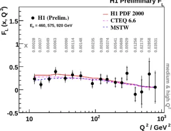
³

-0.5

0 0.5 1

1.5 H1 (Prelim.) H1 PDF 2000 CTEQ 6.6 MSTW

= 460, 575, 920 GeV Ep

0.00028 0.00037 0.00049 0.00063 0.00090 0.00114 0.00148 0.00235 0.00269 0.00374 0.00541 0.00689 0.00929 0.01256 0.02178 0.02858 0.03531

x

H1 Preliminary F

L

2medium & high Q

)

2

(x, Q

L

F

/ GeV

2

Q

2

-0.5 0 0.5 1 1.5

10 10

²

10

³

Figure 3: The measured F

L

(Q

²

) averaged in x at given values of Q

²

. The resulting x values of the averaged F

L

are given in the figure for each point in Q

²

. The curves represent the NLO/NNLO QCD predictions.

The F

L

(Q

²

) values averaged over x at fixed Q

²

are presented in figure 3. The average is performed using the total errors of individual measurements. The overall corre- lated component for the averaged F

L

is estimated to vary between 0.05 and 0.10. The averaged F

L

is compared with the H1 PDF 2000 fit [7] and with the expectations from global parton distribution fit at NNLO (NLO) perturbation the- ory performed by the MSTW [3]

(CTEQ [4]) group and from the NNLO QCD fit by Alekhin [5] (see also figures in [9]). Within the ex- perimental uncertainties the data are consistent with these predic- tions.

4 Summary

The measurement of the longitu- dinal proton structure function in

deep inelastic scattering at low x is presented. The F

L

values are extracted from three sets of cross section measurements at fixed x and Q

²

, but different inelasticity y with three dif- ferent proton beam energies at HERA. For the covered Q

²

range between 12 and 800 GeV

²

, the F

L

results are consistent at the current level of accuracy with the DGLAP evolution framework of perturbative QCD at low x.

References

[1] Slides:

http://indico.cern.ch/contributionDisplay.py?contribId=95&confId=24657

[2] S. Moch, J.A.M. Vermaseren and A. Vogt, Phys. Lett. B606 123 (2005) and references therein.

[3] A.D. Martin, W.J. Stirling, R.S. Thorne and G. Watt, Phys. Lett. B652 292 (2007).

[4] J. Pumplin, H.L. Lai and W.K. Tung, Phys. Rev. D75 054029 (2007);

P.M. Nadolsky et al., arXiv:hep-ph/0802.0007.

[5] S. Alekhin, K. Melnikov, F. Petriello, Phys. Rev. D74 054033 (2006).

[6] C. Adloff et al., H1 Collaboration, Phys. Lett. B393 452 (1997);

C. Adloff et al., H1 Collaboration, Eur. Phys. J. C21 33 (2001).

[7] C. Adloff et al., H1 Collaboration, Eur. Phys. J. C30 1 (2003).

[8] A. Nikiforov, Measurement of the Proton F

L

and F

2

Structure Functions at Low x, 43rd Rencontres de Moriond on QCD and High Energy Interactions, La Thuile, Aosta Valley, Italy (8-15 March 2008);

B. Antunovic, Measurement of the Longitudinal Structure Function F

L

at Low x in the H1 Experiment at HERA, 16th International Workshop on Deep Inelastic Scattering, London (7-11 April 2008);

F.D. Aaron et al., DESY-08-053, accepted for publication in Phys. Lett. B , arXiv:0805.2809.

[9] H1 Collaboration, H1prelim-08-042,

http://www-h1.desy.de/h1/www/publications/htmlsplit/H1prelim-08-042.long.html

DIS 2008