Bending and torsion of thin walled beams with variable, open cross sections

Research Collection

Working Paper

Bending and torsion of thin walled beams with variable, open cross sections

Author(s):

Lonkar, Suresh Publication Date:

1968

Permanent Link:

https://doi.org/10.3929/ethz-a-000747208

Rights / License:

In Copyright - Non-Commercial Use Permitted

This page was generated automatically upon download from the ETH Zurich Research Collection. For more information please consult the Terms of use.

ETH Library

of thin walled

Beams with

variable,

open Cross Sections

Suresh Lonkar

November 1968 Bericht Nr. 18

Institut für Baustatik ETH Zürich

Bending

Beams with

variable,

von

Dr. sc. techn. Suresh Lonkar

Institut für Baustatik

Eidgenössische Technische Hochschule Zürich

Zürich November 1968

Empty

Leer Vide Empty

Empty

The theory ^of thin walled beams with open ^cross section has many applications ⁱⁿ practice, e.g. ⁱⁿ the analysis ^of gir- der bridges. ^{For beams of constant} section Solutions have been available in the technical literature. However, ^few publications exist which deal with beams of variable cross section. In this study ^{a Solution for beams with} unsymmetri-

cal and variable cross section is presented. ^A corresponding Computer program for pratical application ^{has been} developed.

The author has prepared ^this study ⁱⁿ partial fulfilment of his doctoral work at the Institute of Structural Engineering, Department ^{of Civil} Engineering. During ^his stay ^he received

a scholarship ^{of the} Department ^{of the Interior of the Swiss} Federal Government.

Swiss Federal Institute of Technology

Zürich, January ¹⁹⁶⁹

Prof. Dr. B. Thürlimann

Empty

BEAMS WITH VARIABLE OPEN CROSS SECTION

CONTENTS

Page 1. INTRODUCTION:

1.1 Description ^{of the Problem} 9

1.2 Literature Review 9

2. DIFFERENTIAL EQUATIONS ^{AND SOLUTIONS:}

2.1 Differential Equations ^for Bending and Torsion of a thin-walled Beam of constant open Cross

Section 11

2.2 Homogeneous ^{Solutions 15}

2.3 Particular Integrals ¹⁷

2.4 Remarks on the form of the Differential

Equations 18

2.5 Expressions ^{for the Sectional} Forces 19

3. FINITE ELEMENTS METHOD FOR A BEAM OF VARIABLE CROSS SECTION:

3.1 Transport Matrix Method 22

3.2 Transport ^{Matrices for Curved Beams 28}

3.3 Beams of Variable Section 31

3.4 Conditions of Transfer at the Junction of two

Beam Finite Elements 34

3.5 Nature of the Transport Matrix 40

4. SCHEME OF THE COMPUTER PROGRAM 42

5. NUMERICAL EXAMPLES:

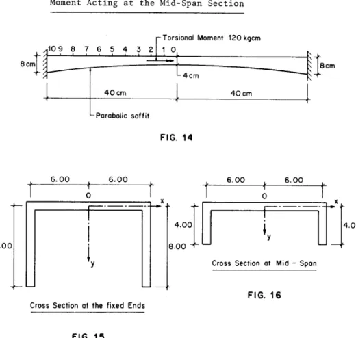
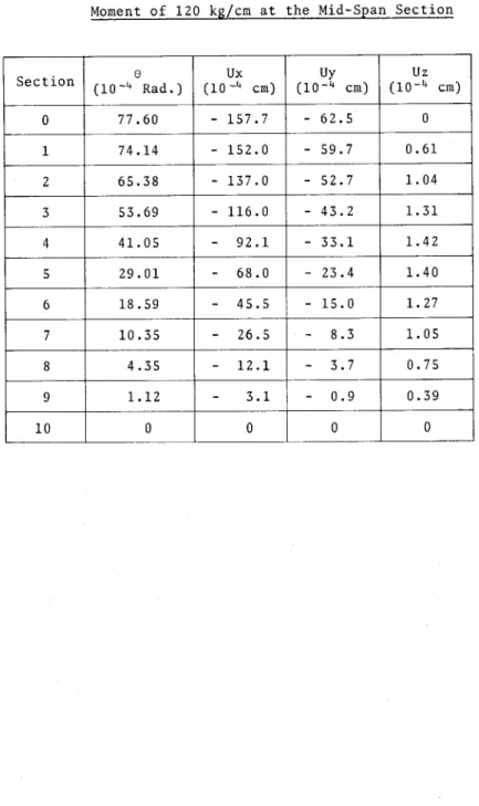
5.1 Fixed Ended Beam with a concentrated Torsional

Moment at the Mid-Span ^Section 44

5.2 Three Span ^{Continuous Beam with a Radial Load}

at Mif'-Span ^Section 54

5.3 Two Span ^{Continuous and} Curved Prestressed

Concrete Bridge 60

6. SUMMARY ₇₁

7. NOTATION 74

8. BIBLIOGRAPHY 80

APPENDIX

1.1 Description ^{of the Problem}

The theory ^{outlined in the} present dissertation aims at the general Solution of the problem ^of bending and torsion of thin walled beams with open ^cross section. The longitudinal axis of the beam _may be straight ^{or curved. The conditions} of support of the beam are arbitrary. ^{The cross section} may be unsymmetrical and variable along ^{the axis.}

1.2 Literature Review

The general problem ^of torsion of thin walled beams with constant open ^cross section has been trated by many authors.

A comprehensive ^{review of the} pertinent ^{literature on the} subject ^of warping ^torsion may be found in the last chapter

of the well-known book by ^{V.Z. Vlassov 1 .}

On the problem of torsion of thin walled beams with variable open section work has been done by ^Z. Cywinski

[21

I 3

J

[4J.

tions of torsion for such beams from the minimum principle of potential energy. He uses the finite difference approach

for the Solution of the differential equations ^{with variable} coefficients. He compares the results of his theoretical So¬

lution with those obtained from tests on a plexi-glass ^model.

Becker considers the equation of torsion of a curved beam of constant monosymmetrical section, ^{as derived} by ^{Vlassov. For} variable sections he imagines ^{the beam to be made} up of short pieces ^{of constant section and uses the Solution} of the sixth order differential equation mentioned earlier. A similar approach ^{for the} analysis of box beams of variable section

has been suggested by Heilig

[5

Both the papers ² and 3 refer to the case of cross sec¬

tions with one axis of symmetry. ^The present ^{work treats the} general ^{case of an} unsymmetrical ^{section. In} paragraphs ^5.1 and 5.2 comparisons ^are made between the Solutions of Cywinski and Becker with those of the present theory.

E. Karamuk

I6J

tion in two parts. In his approach ^{first the St. Venant Tor¬}

sional Rigidity ^is neglected ^and only ^the warping Rigidity is considered. The differential equation ^is then similar to that of plane bending ^{of a beam. Next} only ^{the St. Venant} Rigidity ^{is considered} and the second order homogeneous equation ^{is solved. At discrete} points ^{the two Solutions}

are coupled ^{to fulfill} the conditions of compatibity. ^The redundant forces are then calculated as in the force method.

The Folded Plate Theory ^{is also discussed.}

2. DIFFERENTIAL EQUATIONS ^{AND SOLUTIONS}

2.1 Differential Equations ^of Equilibrium ^{of a Thin}

Walled Beam of Constant Open ^{Cross Section}

FIG. 1

A complete derivation of the differential equation using the arbitrary ^coordinate System may be found in reference

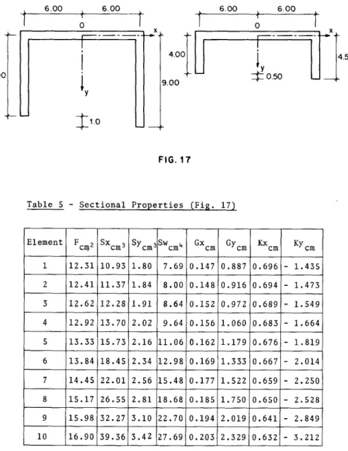
Fig. ^{1 shows an element of a} thin walled beam of open ^cross section. The external loads _qX, q ^, and q act along ^the

y ^z

positive ^{directions of the} x, y, ^{z axes} respectively, ^when looking ^{from the} positive ^{z side. The external torsional mo-}

ment m acts clockwise and the positive ^{direction of the mo-}

ment vector coincides with the positive direction of the z-

axis, consistent with the left handed System ^{of axes x, y,}

z. It may be noted that these are chosen arbitrarily. ^{In the} plane ^{of cross} section, ^{the x} and y ^{axes are} neither the axes of symmetry ^{nor the} principal ^{axes. The s axis is} along

the centre line of the walls of the members and the positive

s direction is in the clockwise sense as seen from the posi¬

tive z side.

The external loads _{q , q} , and _q possess ^the unit kg/cm and the moment ^m kg.cm/cm. ^{T. and} TR ^{are the external shear}

forces acting ^{on the left and} right ^hand edges ^{S = S. and} S ⁼ SR respectively.

Next we consider the deformation of the element under the action of the external loads. The following assumptions ^are made:

1) The material of the beam is elastic. The Stress-Strain relationship ^{is linear.}

2) ^The deformations of the beam are small in comparison with its dimensions. The conditions of equilibrium ^of

the undeformed System ^{are also valid for the deformed} System (first ^order theory).

3) ^{The dimensions of the beam are consistent with the des-} cription ^"thin walled". The normal and shear Stresses are constant over the thickness of each element of the cross section.

4) ^{The cross sectional} shape ^remains unchanged. Hence, under external loads, ^each point ^{in the cross section} undergoes rigid body displacements ^{in the} plane ^{of cross} section. These displacements correspond ^{to three} degrees of freedom, ^{and can be} expressed ^{as functions of:}

a)j The translations U and U of the ^origin of coordinates

x y ^&

0, ^and

b) ^{The rotation 0 of the cross} section with respect ^to the System ^{of axes} x, y, ^z. This is shown in Fig. ^2.

5) During deformation the shear strain of the middle sur- face is relatively ^{small and} hence neglected. ^{Thus a nor¬}

mal to the section remains normal. The warping ^{of the}

cross section before deformation

cross section öfter deformation

FIG. 2

cross section in the direction of the beam axis in de- termined by this condition.

A point ^{P in the cross} section has coordinates _x, y, z, ^w.

The coordinate ^w with the dimensions of an area is defined as follows: See Fig. ^3.

FIG. 3

ds is an elemental are length along ^{the s axis} between ori- gin ^{0 and the} point ^{P and r the} distance between 0 and the tangent ^{to ds. Then}

w ⁼ /rds

0

The point ^{P has three} displacements ^{Ux ,} Uy , and Uz . These

can be expressed in terms of the displacements ^{of the coor¬}

dinate origin ^{0 as follows:}

Uxp ^{= Ux - y 9 (1)} Uyp ^{= Uy + x 9 (2)}

dUx dUy ^dö

Uzpv ⁼ Uz ^{- —-} x ^- —f y ^{- — w} (3)

az dz dz

In equation (3), ^{the first three terms on the} right ^hand side represent plane bending ^{and the last term indicates the} warping ^{of the cross section. This} equation ^can be derived from the condition of zero shear strain of the middle sur- face of the beam, ^{and is} given ^{here without} proof.

In many practical cases, the longitudinal edges ^{of the beam}

are free, ^{and hence the} edge ^{shears T, and TD vanish. The}

L K

differential equations ^of equilibrium may be written as fol¬

lows^:

4

Sw\ ,„ /Iwx\ iv /Iwy\ iv „Tv GK ,2 ., n t-_Iw/ Uz ⁺ \Iw/^{-r—) Ux- +} \Iw/'-z—) Uy- ^{+ 6- - =-}EIw ^{L 6 = -z}E -L

4

(7)

Equations (4) ^to (7) ^{are due to Vlassov} I1I. _They are expres¬

sed here in a slightly ^{different form for} convenience. It may be particularly ^{noted that the} symbol ^' represents the derivative with respect ^to c, whereby ^{c = t is a dimension-}

less parameter, ^L being ^{a reference} length ^{of the beam.}

The various Symbols ^{used in this} paragraph ^{and in all fur-}

ther equations ^are explained ⁱⁿ chapter ^7.

2.2 Homogeneous ^{Solutions of the} System of Differential

Equations

Vlassov lll has given ^{a Solution for a} special ^coordinate system using principle ^{axes reduced to the shear center.}

Here a general Solution for the arbitrary ^coordinate system is presented.

Differentiating equation (4) ^with respect ^to ?, the term L ^• U'"is expressed ^as:

Substituting ^{for L •} U'"in equations (5), (6), ^and (7) these can be rewritten in the following ^form:

a^ ^{Ux— +} a12Uy— ⁺ a13^{8~ =} X2 qx ^- X, g9 qz' (9)

Iv Tv h7 ⁱ

a21 ^{Ux— +} a22^{Uy— +} a236— ⁼ X3 ^{qy -} X, g6 qz (10)

a31^{Ux— +}a32Uy- ⁺a338^{— -} a34e" ⁼ X4 ^m- X, g12 qz' ⁽¹¹⁾

From equation (10)

Tv ^21 Tv Q?^ Tv 1 9g *

Uy- ^{= -—} Ux- ^{- —}8- + X qy ^{- —} X2 ^qz (iz)

a22 o22 a22 a22

This expression ^{for U —is} substituted in equations (9) ^and (11):

b„ ^{Ux- +} b12^{6- =} X2 qx ⁺ X3 b14 qy ^- X, g15 qz' (13)

b21 ^{Ux- +} b22^{6- -} b23 ^{9" =} X4 ^{m +} X3 b24 qy^-X, g16 qz' (14)

From equation (13)

IV °12 „IV X2 . „ b14 9l5

ux- ^{= --^} 8- *

—-q« +x3 -rr^qy-ir^x, qz (15) t>ii &11 t>i1 <>11

This expression for U-Tis substituted in equation (14), which yields ^after rearrangement:

Cn8--C12e" ⁼ X4 ^{m+ y} x2 ^{qx +} g17 X3 ^{qy -} g18 X, qz'

(16) Equation (16) ^{is rewritten in the} following ^form:

8- ^- ß28" ⁼ A m + B qx ⁺C qy ^-D qz' (17)

This is the final differential equation ^{for the} problem ^of bending and torsion of a thin walled beam with constant open section.

The homogeneous ^{Solution for 6 in} equation (17) ^{is of the}

form:

6h ⁼ C, ⁺C2£ ⁺ C3 ^sinhß £ ⁺ C4 ^cosh ß £ (18)

By inspecting (15), the homogeneous ^{Solution for U is ob-} tained as

Uxh ^{= a} flh ⁺C5⁺ C6£ ⁺

C7£2

C8C3

Equation (12) ^{is solved for} Uv ^as:

Uyh ⁼ 910(1 ⁺ 92 Uxn ⁺ C9⁺ C10£+

C^C2

C,2C3

Finally, Integration ^of equation (4) ^{twice with} respect ^to

? yields:

Uzh ⁼ -jj

{(g3öh'+94

j

The Solutions (18) ^to (21) ^{involve 14 constants of Inte¬}

gration ^{C. to C...} They ^{are calculated from the} boundary conditions.

2.3 Particular Integrals

The particular integrals ^{for the} differential equations (17)^, (15)^, (12) ^{, and} (4) ^{can be obtained} straight ^forward when the loadings q ^, q ^, q ^, and ^m are constant ^or known explicitly ^{as continuous functions of} the variable e.

In the following, ^the particular ^{Solutions for} 9, ^U , U ,

x y

and U are given ^{for constant} m, q , q ^, and _q being ^a linear function of c,.

In this _case, the particular integral ^{for e in} equation (17) ^{is obtained} by inspection ^as:

a A -2 B ,2 C D _, .

6P ⁼ ~—2i

m-^? qx-^Iqy+i^Iqz

or

0p ⁼ A0 ^m+ B0 ^{qx +} C0 qy ^- D0 qz' (23)

In the same way equation (15) yields:

Uxp ^{= <x} öp ⁺ o2 £4 qx ⁺ a3 £4 qy ^- a4 £4 qz' (24)

Going ^{back to} equation (12), ^the particular Solution for U is seen to be:

Uyp ⁼ g, ep+g2 Uxp ⁺r, £4 qy ^-r2 £4 qz' ⁽²⁵⁾

Finally ^from equation (4) ^the particular Solution for U is obtained as:

Uzp ⁼

r{<93

(k,£+3k2)]

(26)

The definition of the various Symbols ^is given ⁱⁿ chapter ^7.

The complete ^{Solutions for the} differential equations (4)

to (7), namely ^{for the} displacements ^U , U , U of the co-

x y ^z

ordinate origin 0, ^{and the} angle of rotation 8 of the cross section are thus as follows:

8 ⁼ en ⁺Sp ^— Equations(18) ^and (23) Ux ⁼ Uxn ⁺Uxp ^— Equations(19) ^and (24) Uy ⁼ Uyn ⁺ Uyp ^— Equations (20) ^and (25)

Uz ⁼ Uzn ⁺Uzp ^— Equations(21) ^{and (26)}

2.4 Remarks on the Form of the Differential Equations

Referring ^to equations (4) ^to (7), ^the following points ^be noted:

Equation (4) expresses the equilibrium ^{of the internal} and external forces along ^{the z or} longitudinal ^axis.

Equation (5) refers to bending ^{in the xz} plane. ^{The ben¬}

ding ^{of the element in} the yz plane ^is expressed by equa¬

tion (6). ^The equilibrium of the external and internal torsional moments is contained in differential equation (7).

In the case of a beam with two axes of symmetry, ^{if x} and y ^are the principal axes, equations (4), (5), (6), ^and (7) contain terms only ^{in U , U , U , and 0} respectively. ^The coefficients of the other terms, ^for example ^{of U , U ,}

j

x y

and g in equation (4), ^{would vanish. The Solutions for}

U , U , U , and 9 will then be independant of eachother.

In a particular problem ^this would be automatically ^taken

care of in Solutions (18) ^to (21) ^and (23) ^to (26).

Choosing ^the x, y, and ^z axes arbitrarily ^{and then} getting the Solutions for the displacements ^{of the} arbitrary ^ori¬

gin 0, namely ^{U , U , U and the rotation 9 of the cross} section leads to a Solution for the general problem ^of bending and torsion of a thin walled beam of unsymmetri-

cal open ^cross section.

2.5 Expressions ^{for the} Sectional Forces

In paragraphs2.2 ^{and 2.3 Solutions were} obtained for U ,

U , U _, and 9, ^which satisfy ^the differential equations (4)

y ^z

to (7). ^{The internal} forces acting ^{on a cross section can}

now be expressed ^as functions of the derivates of these

displacements.

Referring ^to Fig. ^{4 the basic} expressions ^{for the normal} and shear Stresses at a point ^P with coordinates x, y, z, s> ^w are as follows:

(x,y,z,s,w)

FIG. 4

follows:

P F (s) ^-

/dF

0 P Sx(s) ⁼

J

Normal Stress:

6 ⁼

-jj(L

Shear Stress:

T ⁼

^(-^)

Uz"+^ Ux'"+^ Uy'".^ ö'")

(28)

The quantities F(s), ^S (s), ^S (s), ^{and S} (s) ^{are defined as}

P

Sy(s) ⁼

/ydF

Q P Sw(s) ⁼

J

Q Q

The point Q ^{lies on the free} edge ^{where the shear stress} vanishes. While going ^from Q ^{to P} along ^{the centre line of} the wall the movement is in the positive ^{s sense. i.e.}

clockwise.

The sectional forces are defined as follows:

1) Normal force N ⁼

J

F

2) Bending ^Moment My ⁼

-J

F

3) Bending ^{Moment Mx =}

J

F

4) Warping ^{Moment Mw =} J ^SwdF

F

5) Shear Force Qx ⁼

/(Tt)dx

S

6) Shear Force Qy ⁼

J

7) Torsional Moment T ⁼

J

Where Warping ^{Torsional Moment Ts = — 8'}

St. Venant Torsional Moment Tw ⁼ / (rt)dw

On using equations (27) ^and (28) ^and carrying ^{out the inte-} grations, ^the following expressions ^{are obtained for the} Section Forces:

N ⁼

-^|-

Mx ^{= ~} (L g6 Uz'-g7 ^{Ux" - Uy"-} g8 e") (30)

My ⁼

-^

EIw , „ „

Mw ⁼

-j-j- ^{(L g12 Uz - g13 Ux -g14 Uy - 8 ) (32)}

Ts ^{= ——} 6 (33a)

T« ⁼

^y

L3

EIw .i in ,,,

Ts⁺ Tw ^{= ——}(g12 ^{L Uz -}g13 ^{Ux -}g14 Uy ^{- 8 +}<j>, ^{8' )}

E I (33)

Qx ^{= ~} (L _g9 Uz" -Ux"'-g10 Uy"'-g,, 8"') (34)

Qy ⁼ -[J ^{(L g6} Uz"-g7 Ux'"-Uy'"-g8 ^{9'") —¦ (35)}

The various Symbols ^{used are} explained ⁱⁿ chapter ^{7. In} the appendix ^a matrix representation ^{of relations} (29) ^to (35) ^is given.

3. THE FINITE ELEMENTS METHOD FOR BEAMS OF VARIABLE

SECTION

3.1 The Transport ^{Matrix Method}

This method is discussed for Beam Bending problems by Zurmühl 7 ^. Still, the essentials will be presented ^here for the sake of clarity ^{with the} help ^{of a} simple ^illustra¬

tive example. ^{In the} following simple bending ^{of a canti-} lever beam is considered.

El ⁼ constant

T"

FIG. 5

Fig. ^{5 shows a cantilever beam LR of} length ^{a. The beam is} prismatic ^{and its cross} section has two axes of symmetry x, and _y. It carries a concentrated load P at the free end R.

Using ^the transport matrix method the bending ^{moment and} the shear force at the fixed end L and the slope ^{and verti-} cai deflection at the free end R are to be calculated.

The Differential Equation of equilibrium ^{in the} plane yz of the load is:

d4 Uy d-C«

qy o^

E I * ⁼ ö

The Solution for Uis

Uy ^{= A+} B£ ⁺

C£2+D£3

A, B, C, ^D being ^{the constants of} Integration

Slope dUy

dz 1 «ü* =

1[B+C

a d£ ^{a L J}

2 2

Bending ^{Moment M = -E I}^-^ ^=- ^| ^-^ ^{= -} ^ [2C+6D£l

dz2 a2 d£2 a2 ^{l J}

(38)

o. n dM 1 dM EI „

Shear Force Q ^{= -— = —} -r—= ^- 6D

dz a d£ ^a3 (39)

Equations (36) ^to (39) ^{are written} in Matrix form as follows

Uy

a d£

M

1 c £2 C3 ^A

0 1

a

2£

a

3«!

a

B

0 0 2EI

"

a2 a2 ^{g C}

0 0 0 6EI

"

a3 ^{- D}

(40)

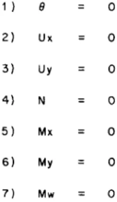
Boundary Conditions

a) Free End £ ⁼ 0, 1) M ⁼ 0, 2) ^{Q = -P}

b) Fixed End £ ^{= 1} , 3) Uy ⁼ 0, 4) ^-

^

For a particular value of , the quantities ^{on the left} hand side of equation (40) ^{constitute a vector called the}

"State Vector".

The State Vector

[SR1

w

U/R

1 /dUy'/dUy\

Vd£/R

a\d£

0

-P

10 0 0

0-00a

0

0-^0

a2

0 0 0 ^--6EI

(41)

In Matrix notation equation (41) ^{is written as}

[SR]

[x]

[COM]

Here

IXJ

equation (41) , and I

CONJ

of Integration A, B, C, ^D.

Similarly, ^{the State Vector at the fixed end L is} given by:

[SL]

"

a2 a2

0 ^-6EI

Or in Matrix notation:

[sL]

[y]

[CON]

Premultiplying ^{both sides of} equation (42) by ^{the inverse} matrix

|x|-1,

[CON]

[x]"1- [SR]

Substituting ^this expression ^{for the vector} [CONJ ^{in equa¬}

tion (43):

N

W-WM8»]

[TR]LR

[SR]

In equation (45) ^the "Transport Matrix"

[tr1r

m*

m

[*r

X being ^a diagonal matrix,

Inverse Matrix

[»r

10 0 0

0 a 0 0

2E1

0 -:

6EI

146)

By ^{the rules of Matrix} multiplication, ^the Transport ^Matrix

[tr]

Mi

0 1

"2EI 6EI

EI 2EI

0 0 1a

0 0 0 1

|L

(47)

Substituting ^this expression ^for [tr]r, ^Matrix equation (45) ^{is rewritten as:}

0

0

1

0

Equation (48) yields:

O2 g3

°

2EI 6EI

1 °- ^°2

"EI 2EI

UyR l/dUy\

aVd£yR

-P

(48)

(Uy)R

1_/dUy\

a\d£/fl

-Pa

Po3

3EI

_ p02 2EI

The results are consistent with the chosen sign Convention.

This method is now extended to the problem ^of bending ^and torsion of thin walled beams. In this case the State Vector has fifteen rows. These are:

The seven Deformations:

Ux, Ux', Uy, Uy', Uz, fl, ^and ö'

The seven Section Forces:

N, Mx, My, Qx, Qy, T, ^{ond Mw}

and the term Unity which takes care of the particular ^Solu¬

tions and their derivatives in the matrix Operations.

For the sake of convenience, ^{the above} quantities, namely the Deformations and Section Forces are multiplied by ^sui- table multipliers ^to get ^well conditioned transport ^matrices.