Off-diagonal correlators of conserved charges from lattice QCD and how to relate them to experiment

Off-diagonal correlators of conserved charges from lattice QCD and how to relate them to experiment

R. Bellwied

Department of Physics, University of Houston, Houston, Texas 77204, USA S. Borsányi

University of Wuppertal, Department of Physics, Wuppertal D-42119, Germany Z. Fodor

University of Wuppertal, Department of Physics, Wuppertal D-42119, Germany Eötvös University, Budapest 1117, Hungary, Jülich Supercomputing Centre, Jülich D-52425, Germany, and UCSD,

Physics Department, San Diego, California 92093, USA J. N. Guenther

University of Wuppertal, Department of Physics, Wuppertal D-42119, Germany and University of Regensburg, Department of Physics, Regensburg D-93053, Germany

J. Noronha-Hostler

Department of Physics, University of Illinois at Urbana-Champaign, Urbana, Illinois 61801, USA P. Parotto ^*

Department of Physics, University of Houston, Houston, Texas 77204, USA and University of Wuppertal, Department of Physics, Wuppertal D-42119, Germany

A. Pásztor

Eötvös University, Budapest 1117, Hungary C. Ratti and J. M. Stafford

Department of Physics, University of Houston, Houston, Texas 77204, USA

(Received 12 November 2019; accepted 22 January 2020; published 10 February 2020) Like fluctuations, nondiagonal correlators of conserved charges provide a tool for the study of chemical freeze-out in heavy ion collisions. They can be calculated in thermal equilibrium using lattice simulations, and be connected to moments of event-by-event net-particle multiplicity distributions. We calculate them from continuum-extrapolated lattice simulations atμB¼0, and present a finite-μBextrapolation, comparing two different methods. In order to relate the grand canonical observables to the experimentally available net- particle fluctuations and correlations, we perform a hadron resonance gas model analysis, which allows us to completely break down the contributions from different hadrons. We then construct suitable hadronic proxies for fluctuation ratios, and study their behavior at finite chemical potentials. We also study the effect of introducing acceptance cuts, and argue that the small dependence of certain ratios on the latter allows for a direct comparison with lattice QCD results, provided that the same cuts are applied to all hadronic species.

Finally, we perform a comparison for the constructed quantities for experimentally available measurements from the STAR Collaboration. Thus, we estimate the chemical freeze-out temperature to 165 MeV using a strangeness-related proxy. This is a rather high temperature for the use of the hadron resonance gas; thus, further lattice studies are necessary to provide first principle results at intermediateμB.

DOI:10.1103/PhysRevD.101.034506

*Corresponding author.

parotto@uni-wuppertal.de

Published by the American Physical Society under the terms of theCreative Commons Attribution 4.0 Internationallicense. Further distribution of this work must maintain attribution to the author(s) and the published article’s title, journal citation, and DOI. Funded by SCOAP³.

I. INTRODUCTION

The study of the phase diagram of quantum chromody- namics (QCD) has been the object of intense effort from both theory and experiment in the last decades. Relativistic heavy ion collision experiments both at the Relativistic Heavy Ion Collider (RHIC) and the Large Hadron Collider (LHC) have been able to create the quark gluon plasma (QGP) in the laboratory, and explore the low-to-moderate baryon density region of the QCD phase diagram.

At low baryon density, the transition from a hadron gas to a deconfined QGP was shown by lattice QCD calcu- lations to be a broad crossover[1]atT≃155MeV[1–4].

At large baryon densities, the nature of the phase transition is expected to change into first order, thus implying the presence of a critical end point. A strong experimental effort is currently in place through the second Beam Energy Scan (BES-II) program at the RHIC in 2019–2021, with the goal of discovering such a critical point.

The structure of the QCD phase diagram cannot cur- rently be theoretically calculated from first principles, as lattice calculations are hindered by the sign problem at finite density. Several methods have been utilized in order to expand the reach of lattice QCD to finite density, like full reweighting [5], Taylor expansion of the observables around μB¼0 [6–10], or their analytical continuation from imaginary chemical potential [5,11–14].

We remark here that there are alternative approaches to lattice QCD for the thermodynamical description. Specific truncations of the Dyson-Schwinger equations allow the calculation of the crossover line and also to extract baryonic fluctuations [15,16]. Another theoretical result on the baryon-strangeness correlator has been calculated using functional methods from the Polyakov-loop-extended quark meson model in[17,18].

The confined, low-temperature regime of the theory is well described by the hadron resonance gas (HRG) model, which is able to reproduce the vast majority of lattice QCD results in this regime[19–24]. Moreover, the HRG model has been extremely successful in reproducing experimental results for particle yields over several orders of magnitude [25–29]. These are usually referred to as thermal fits, since the goal of the procedure is the determination of the temperature and chemical potential at which the particle yields are frozen. This moment in the evolution of a heavy ion collision is called chemical freeze-out, and takes place when inelastic collisions within the hot hadronic medium cease. The underlying assumption is that the system produced in heavy ion collisions eventually reaches thermal equilibrium[30–32], and therefore a comparison between thermal models and experiment is possible[33].

Although the net number of individual particles may change after the chemical freeze-out through resonance decays, the net baryon number, strangeness and electric charge are conserved. Their event-by-event fluctuations are expected to correspond to a grand canonical ensemble. In

general, when dealing with fluctuations in QCD, and in particular in relation to heavy ion collisions, it is important to relate fluctuations of such conserved charges and the event-by-event fluctuations of observed (hadronic) species.

The former have been extensively studied with lattice simulations[34–43], and are essential to the study of the QCD phase diagram for multiple reasons. First, they are directly related to the Taylor coefficients in the expansion of the pressure to finite chemical potential and have been utilized to reconstruct the equation of state of QCD at finite density, both in the case of sole baryon number conserva- tion [41,44,45], and with the inclusion of all conserved charges [46]. Second, higher order fluctuations are expected to diverge as powers of the correlation length in the vicinity of the critical point, and have thus been proposed as natural signatures for its experimental search [47,48]. On the other hand, fluctuations of observable particles can be measured in experiments, and are very closely related to conserved charge fluctuations. With some caveats [49–52], comparisons between the two can be made, provided that certain effects are taken into account.

Previous studies found that, for certain particle species, fluctuations are more sensitive to the freeze-out parameters than yields[53]. In recent years, the STAR Collaboration has published results for the fluctuations of net proton[54], net charge[55], net kaon[56], and more recently netΛ[57]

and for correlators between different hadronic species [57,58]. From the analysis of net-proton and net-charge fluctuations in the HRG model, it was found that the obtained freeze-out temperatures are lower than the corre- sponding ones from fits of the yields [52]. More recent analyses[59,60]of the moments of net-kaon distributions showed that it is not possible to reproduce the experimental results for net-kaon fluctuations with the same freeze-out parameters obtained from the analysis of net proton and net charge. In particular, the obtained freeze-out temperature is consistently higher, with a separation that increases with the collision energy. In[59], predictions for the moments of net-Λdistributions were provided, calculated at the freeze- out of net kaons and net proton/net charge.

Correlations between different conserved charges in QCD provide yet another possibility for the comparison of theory and experiment. They will likely receive further contribution from measurements in the future, with new species being analyzed and increased statistics allowing for better deter- mination of moments of event-by-event distributions[58].

In this manuscript, we present continuum-extrapolated lattice QCD results for all second-order nondiagonal corre- lators of conserved charges. We then identify the contribu- tion of the single particle species to these correlators, distinguishing between measured and nonmeasured species.

Finally, we identify a set of observables, which can serve as proxies to measure the conserved charge correlators. The manuscript is organized as follows. In Sec.IIwe present the continuum extrapolated lattice results for second-order

nondiagonal correlators of conserved charges and discuss the extrapolation to finiteμBin Sec.III. In Sec.IVwe show the comparison with HRG model calculations, and describe the breakdown of the different contributions to the observ- ables shown in the previous section. In Sec.Vwe propose new observables which can serve as proxies to directly study the correlation of conserved charges. In Sec.VIwe analyze the behavior of the constructed proxies at finite chemical potential, and study the effect of acceptance cuts in the HRG calculations. We argue that the small dependence on experimental effects allows for a direct comparison with lattice QCD results. We also perform a comparison to experimental results for selected observables in Sec. VII.

Finally, in Sec. VIIIwe present our conclusions.

II. LATTICE QCD AND THE GRAND CANONICAL ENSEMBLE

The lattice formulation of quantum chromodynamics opens a nonperturbative approach to the underlying quantum field theory in equilibrium. Its partition function belongs to a grand canonical ensemble, parametrized by the baryochem- ical potentialμ_B, the strangeness chemical potentialμ_Sand the temperatureT. Additional parameters include the volume L³, which is assumed to be large enough to have negligible volume effects, and the quark masses. The latter control the pion and kaon masses, and are set to reproduce their physical values. At the level of accuracy of this study we can assume the degeneracy of the light quarksmu¼mdand neglect the effects coming from quantum electrodynamics.

There is a conserved charge corresponding to each flavor of QCD. The grand canonical partition function can be then written in terms of quark number chemical potentials (μ_u, μ_d,μ_s). The derivatives of the grand potential with respect to these chemical potentials are the susceptibilities of quark flavors, defined as

χ^u;d;s_i;j;k ¼ ∂^iþjþkðp=T⁴Þ

ð∂μˆ_uÞⁱð∂μˆ_dÞ^jð∂μˆ_sÞ^k; ð1Þ with μˆ_q¼μ_q=T. These derivatives are normalized to be dimensionless and finite in the complete temperature range.

For the purpose of phenomenology we introduce for theB (baryon number),Q(electric charge) andS(strangeness) a chemical potentialμB,μQandμS, respectively. The basis of μ_u, μ_d, μ_s can be transformed into a basis of μ_B, μ_Q, μ_S using the B, QandScharges of the individual quarks,

μu¼1 3μBþ2

3μQ; ð2Þ

μd¼1 3μB−1

3μQ; ð3Þ

μ_s¼1 3μ_B−1

3μ_Q−μ_S: ð4Þ

Susceptibilities are then defined as

χ^BQS_ijk ðT;μˆ_B;μˆ_Q;μˆ_SÞ ¼∂^iþjþkðpðT;μˆB;μˆQ;μˆSÞ=T⁴Þ

∂μˆⁱ_B∂μˆ^j_Q∂μˆ^k_S : ð5Þ It is straightforward to express the derivatives of p=T⁴ with respect toμ_B,μ_Qandμ_Sin terms of the coefficients in Eq.(1) [36,39,61]. For the cross-correlators we have

χ^BQ₁₁ ¼1

9½χ^u₂−χ^s₂−χ^us₁₁þχ^ud₁₁; ð6Þ χ^BS₁₁ ¼−1

3½χ^s₂þ2χ^us₁₁; ð7Þ χ^QS₁₁ ¼1

3½χ^s₂−χ^us₁₁: ð8Þ Such derivatives play an important role in experiment. In an ideal setup the mean of a conserved charge i can be expressed as the first derivative with respect to the chemical potential,

hN_ii ¼T∂logZðT; V;fμ_qgÞ

∂μi

; ð9Þ

while fluctuations and cross-correlators (say between chargesi andj) are second derivatives,

∂hNii

∂μj

¼T∂²logZðT; V;fμqgÞ

∂μj∂μi

¼1

TðhN_iN_ji−hN_iihN_jiÞ:

ð10Þ In these formulasN_i indicates the net number of charge carriers. For example, for the baryon numberB, it corre- sponds to the number of baryons minus the number of antibaryons.

The procedure to define the chemical potential on the lattice[62] and to extract the derivatives in Eq. (1) from simulations that run atμ_u¼μ_d¼μ_s¼0has been worked out long ago[6]and has been the basis of many studies ever since[7,61,63,64]. Since the derivatives with respect to the chemical potential require no renormalization, a continuum limit could be computed as soon as results on sufficiently fine lattices emerged [3,36]. Later the temperature range and the accuracy of these extrapolations were extended in[39,40].

In this work, we extend our previous results [39] to nondiagonal correlators and calculate a specific ratio that will be later compared to experiment.

These expectation values are naturally volume depen- dent. Their leading volume dependence can, however, be canceled by forming ratios. In[37,38,65]such ratios were formed between various moments of electric charge fluc- tuations, and also for baryon fluctuations. For the same ratios the STAR experiment has provided proxies as part of the Beam Energy Scan I program[54,55].

The gauge action is defined by the tree-level Symanzik improvement, and the fermion action is a one link staggered with four levels of stout smearing. The parameters of the discretization as well as the bare couplings and quark masses are given in[39].

The charm quark is also included in our simulations, in order to account for its partial pressure at temperatures above 200 MeV, where it is no longer negligible[66]. In the range of the expected chemical freeze-out temperature between 135 and 165 MeV the effect of the charm quark is not noticeable on the lighter flavors [39].

In this work we use the lattice sizes of32³×8,40³×10, 48³×12,64³×16as well as80³×20. Thus, the physical volumeL³is given in terms of the temperature asLT¼4 throughout this paper. The coarsest lattice was never in the

scaling region. The finest lattice lacks the precision of the others, and we only use it when the coarser lattices, e.g., 40³×10, are not well in the scaling region and if, for a particular observable, the80³×20has small enough error bars. If this was used, the data set is also shown in the plots.

We show here the continuum extrapolated cross-corre- lators at zero chemical potential. In Fig. 1 we show an example of continuum extrapolation for the three cross- correlators, with T ¼150MeV and the w0-based scale setting[67]. Figure2showsχ^BQ₁₁ðTÞ for the four different lattices, as well as the continuum extrapolation. Although our simulation contains a dynamical charm quark, we did not account for its baryon charge. Thus, the Stefan- Boltzmann limit of this quantity is 0. This limit is reached when the mass difference between the strange and light quarks becomes negligible in comparison to the temper- ature. The peak is seen at a higher temperature than Tc≈155MeV, while in the transition region there is an inflection point. BelowT_c this correlator is dominated by protons and charged hyperons. In Sec.IV we account in detail for various hadronic contributions in the con- fined phase.

-0.1 -0.05 0 0.05 0.1 0.15

0 0.004 0.008 0.012 0.016

1/N_t² T=150 MeV

χ^QS11 χ^BS11 χ^BQ11

FIG. 1. Examples for the continuum extrapolation. We show the three cross-correlators on the lattices (from right to left):32³× 8,40³×10,48³×12,64³×16 and 80³×20. The data points correspond to the w₀-based scale setting[67], one of the two interpolation methods to align all simulation results to the same temperature:T¼150 MeV in this example. The error bars in the continuum limit are obtained from the combination of the scale setting, the interpolation, the selection of the continuum extrapo- lation fit range, and whether a linear or 1/linear function is fitted.

0.000 0.005 0.010 0.015 0.020 0.025 0.030 0.035

135 140 145 150 155 160 165 170 175 180 185 190 χ^BQ11

T [MeV]

continuum extrapolaiton 40³x10 lattice 48³x12 lattice 64³x16 lattice 80³x20 lattice

FIG. 2. The baryon-electric charge cross correlator from the lattice at finite lattice spacing and its continuum limit.

-0.20 -0.15 -0.10 -0.05 0.00

135 140 145 150 155 160 165 170 175 180 185 190 χ^BS11

T [MeV]

continuum extrapolaiton 40³x10 lattice 48³x12 lattice 64³x16 lattice

FIG. 3. The baryon-strangeness cross correlator from the lattice at finite lattice spacing and its continuum limit.

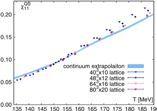
0.00 0.05 0.10 0.15 0.20

135 140 145 150 155 160 165 170 175 180 185 190 χ^QS11

T [MeV]

continuum extrapolaiton 40³x10 lattice 48³x12 lattice 64³x16 lattice 80³x20 lattice

FIG. 4. The electric charge-strangeness cross correlator from the lattice at finite lattice spacing and its continuum limit.

Theχ^BS₁₁ðTÞcorrelator is shown in Fig.3. Unlike theBQ correlator, we have now a monotonic function with a high temperature limit of−1=3, which is the baryon number of the strange quark. The transition has a remarkably small effect on this quantity. At low temperatures this correlator is basically the hyperon free energy.

The χ^QS₁₁ðTÞ correlator in Fig. 4 is also monotonic, converging to 1=3 at highT, which is the electric charge of the strange quark. At low temperatures this quantity is dominated by the charged kaons, which were the focus of recent experimental investigations[56].

The continuum-extrapolated results at μ_B¼0 for χ^BQ₁₁, χ^BS₁₁, χ^QS₁₁ and the ratio χ^BS₁₁=χ^S₂ we discuss below are provided in TableI of the Appendix.

III. RESULTS AT FINITE DENSITY

Since lattice QCD can be defined at finite values of theB, Q andSchemical potentials, and is capable of calculating derivatives of the free energy as a function of these chemical potentials one could expect that the extension of the simulations to finite density is a mere technical detail.

Unfortunately, at any finite real value of the quark chemical potentialμ_qthe fermionic contribution to the action becomes complex and most simulation algorithms break down.

There are several options to extract physics at finite densities, nevertheless. It seems natural to use algorithms that were designed to work on complex actions—both the complex Langevin equation[68]and the Lefschetz thimble approach[69]have shown promising results recently—yet their direct application to phenomenology requires further research.

Instead, we use here the parameter domain that is available for mainstream lattice simulations. In fact, besides zero chemical potential, simulations at imaginary μB are also possible, and have been exploited in the past to extrapolate the transition temperature[70–73], fluctuations of conserved charges[42,43]and the equation of state[41].

In all these works it was assumed that the thermodynamical observables are all analytical functions of μˆ²_B.

A conceptually very similar method, the Taylor method, provides the extrapolation in terms of calculating higher derivatives with respect toμˆ_B. The series is truncated at a certain order, which is typically limited by the statistics of the lattice simulation.

Since we relate the baryon-strangeness correlator to experimental observables later on we useχ^BS₁₁ as an example for the Taylor expansion,

χ^BS₁₁ðT;μÞ ¼ˆ χ^BS₁₁ðT;0Þ þμˆ_Bχ^BS₂₁ðT;0Þ þμˆ_Sχ^BS₁₂ðT;0Þ þμˆ²_B

2 χ^BS₃₁ðT;0Þ þμˆ_Bμˆ_Sχ^BS₂₂ðT;0Þ þμˆ²_S

2 χ^BS₁₃ðT;0Þ þOðˆμ⁴Þ; ð11Þ

where the terms proportional toμˆBandμˆSvanish since they contain odd derivatives, which are forbidden by the C-symmetry of QCD. (The charge chemical potential is omitted for simplicity).

In most phenomenological lattice studies the chemical potentials are selected such that the strangeness vanishes for each set ofðμB;μQ;μSÞ. More precisely, for eachTand ˆ

μB we select μˆQ and μˆS values such that χ^S₁ðT;fˆμ_igÞ ¼0;

χ^Q₁ðT;fμˆ_igÞ ¼0.4χ^B₁ðT;fˆμ_igÞ: ð12Þ The factor 0.4 is the typicalZ=A ratio for the projectiles in the heavy ion collision setup, and the value we use in the HRG model calculations below. In our lattice study, however, we use 0.5. This introduces a small effect com- pared to the statistical and systematic errors of the extrapo- lation, and results in substantial simplification of the formalism: μ_Q can be chosen to be 0. The would-be μ_Q value is about one tenth ofμSin the transition region[37,38].

We checked the impact of our simplification on the results we present here, with the Taylor expansion method. Utilizing our simulations data from ensembles atμB¼0, we calculate the correction to the ratio χ^BS₁₁=χ^S₂. By construction, this correction vanishes atμ_B ¼0, and we find that it grows to at most 1% atμ_B=T¼1, and at most 1.5% atμ_B=T¼2. These systematic errors are considerably smaller than the uncer- tainties we have on our results, as can be seen in Fig.5.

A. Taylor method

The Taylor coefficients for correlators can be easily obtained by considering the higher derivatives with respect toμB. For later reference we select the quantityχ^BS₁₁=χ^S₂for closer inspection,

χ^BS₁₁ χ^S₂

μB=T

¼χ^BS₁₁ χ^S₂ þμˆ²_B

2

χ^BS;ðNLOÞ₁₁ χ^S₂−χ^S;ðNLOÞ₂ χ^BS₁₁

ðχ^S₂Þ² ; ð13Þ up toOðˆμ⁴_BÞ corrections, with

χ^BS;ðNLOÞ₁₁ ¼χ^BS₁₃s²₁þ2χ^BS₂₂s1þχ^BS₃₁; ð14Þ χ^S;ðNLOÞ₂ ¼χ^BS₂₂ þ2χ^BS₁₃s1þχ^S₄s²₁; ð15Þ s1¼−χ^BS₁₁=χ^S₂: ð16Þ The derivatives on the right-hand side are all taken at μB¼μS¼0.

Whether we extract the required derivatives from a single simulation (one per temperature) at μ_B ¼μ_S¼0 or we determine the fourth order derivatives numerically by the (imaginary)μ_B-dependence of second-order derivatives is a result of a cost benefit analysis. The equivalence of these two choices has been shown on simulation data (of the

chemical potential dependence of the transition temper- ature) in[73].

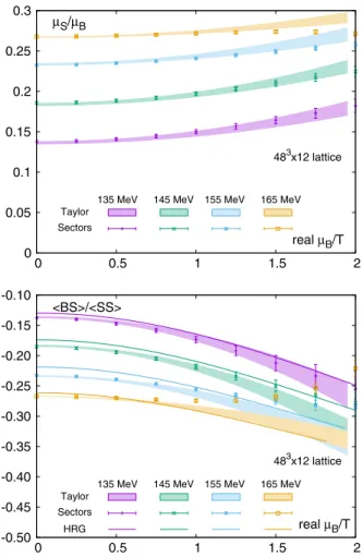
In [71] we calculated direct derivatives; however, we obtained smaller errors by using imaginaryμ_B simulations in[43]. Thus, we take the Taylor coefficients from the latter analysis, now extended to the new observable. The results for several fixed temperatures are shown in Fig.5. As a first observable we show theμS=μB ratio that realizes strange- ness neutrality. Then we show theχ^BS₁₁=χ^S₂ratio as a function of positive μˆ²_B.

In the plots we show results from a specific lattice 48³×12, which has the highest statistics, so that it pro- vides the best ground to compare different extrapolation strategies.

B. Sector method

In Fig.5we compare two extrapolation strategies; here we describe the second approach, the sector method.

We are building on our earlier work in[74], where we have written the pressure of QCD as a sum of the sectors Pðμˆ_B;μˆ_SÞ ¼P^BS₀₀ þP^BS₁₀ coshðˆμ_BÞ þP^BS₀₁ coshðμˆ_SÞ

þP^BS₁₁ coshðμˆB−μˆSÞ þP^BS₁₂ coshðμˆ_B−2μˆ_SÞ

þP^BS₁₃ coshðμˆ_B−3μˆ_SÞ: ð17Þ These sectors were also studied in [75,76]. Obviously, QCD receives contributions from sectors with higher quantum numbers as well. The sectors in Eq. (17) are the only ones receiving contributions from the ideal hadron resonance gas model in the Boltzmann approximation. (The dependence on the electric charge chemical potential is not considered now, since we selectedμ_Q ¼0.)

The partitioning of the QCD pressure in sectors is very natural in the space of imaginary chemical potentialsμˆ_B¼ iˆμ^I_B andμˆ_S¼iμˆ^I_S,

Pðμˆ^I_B;μˆ^I_SÞ ¼X

j;k

P^BS_jk cosðjμˆ^I_B−kˆμ^I_SÞ: ð18Þ It is expected that higher sectors are increasingly relevant as Tc is approached from below. A study using Wuppertal- Budapest simulation data has shown that below T≈ 165MeV the sectors jBj ¼0, 1, 2 give a reasonable description, e.g., by calculating χ^B₄ from the sector coef- ficients and comparing to direct results.

Thus, for this work we considered the next-to-leading order of the sector expansion, including the

LO∶P^BS₀₁; P^BS₁₁; P^BS₁₂; P^BS₁₃;

NLO∶P^BS₀₂; P^BS_1;−1; P^BS₂₁; P^BS₂₂: ð19Þ It is somewhat ambiguous how theNLOis to be defined.

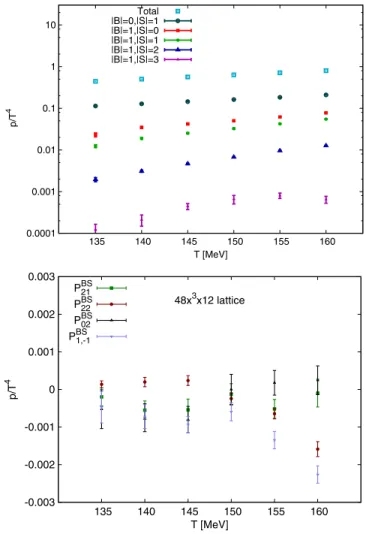
One option would be to include the next-higher jBj quantum number, making our approach second order in this expansion. We do include P^BS₂₁ and P^BS₂₂; however adding further higher strangeness sectors, e.g., P^BS₂₃, did not improve the agreement with our data, so it was not included. Moreover, we included the multistrange sector P^BS₀₂ and the exotic sectorP^BS_1;−1, which is the coefficient of the term proportional to coshðμˆ_Bþμˆ_SÞ. On the other hand, removing the sectors included in theNLOnever resulted in higher temperatures in a smallerχ²for the fit; e.g., atT¼ 160MeV removing the termsP^BS_0;2,P^BS_1;−1P^BS_2;1orP^BS_2;0from the fit (removing only one term at a time) resulted in a χ²=N_dof of 72.6=53, 181.1=53, 72.4=53, or 137.2=53, respectively, while including all gave72.3=52.

In Fig.6the results for the sectors in theLOandNLO are shown at different temperatures. The results for theLO sectors shown in the top panel (figure from Ref.[74]) are continuum extrapolated—except for the jBj ¼0, jSj ¼1

0 0.05 0.1 0.15 0.2 0.25 0.3

0 0.5 1 1.5 2

real μB/T μS/μB

135 MeV 145 MeV 155 MeV 165 MeV Taylor

Sectors

48³x12 lattice

-0.50 -0.45 -0.40 -0.35 -0.30 -0.25 -0.20 -0.15 -0.10

0 0.5 1 1.5 2

real μB/T

<BS>/<SS>

135 MeV 145 MeV 155 MeV 165 MeV Taylor

Sectors HRG

48³x12 lattice

FIG. 5. Comparison of two approaches to the finite density extrapolation of two observables. The Taylor result is truncated such that only the leading∼ˆμ²Bcontribution is considered. In the sector method, contributions up to jBj ¼2 are included. (The data were generated from a48³×12lattice; the plots show the intermediate result before continuum extrapolation.) We also show the hadron resonance gas model prediction.

sector. In the lower panel new results for the sectors in the NLO are shown, generated from a48³×12lattice.

The alert reader may ask why we do not include theP^BS₁₀ sector, accounting e.g., for protons. In fact, the sectors with jSj ¼0do not contribute to the observablesχ^BS₁₁,χ^S₂ orχ^S₁ either at 0, or at any real or imaginary chemical potential. In the analysis we included results forχ^S₁,χ^S₂,χ^BS₁₁ from various data sets at various imaginary chemical potentials: at μ_B ¼0, μ_S¼0 the data of Sec. II, the μ^I_B >0, μ_S¼0 data set of [43], the strangeness data set with μ^I_B>0 of [41], and finally the set (only including χ^S₁ and χ^S₂) with μ_B ¼0,μ^I_S>0from [74]. For the lower temperatures the model defined with the coefficients in Eq.(19)resulted in good fits (Qvalues ranging from 0 to 1)—the worst fit was at T¼165MeV with Q≈0.05. This is the temperature where the model is expected to break down.

Now we can compare the results to the Taylor expansion.

In Fig.5we show the sector results with error bars, while the bands refer to the Taylor method. At low temperatures we see good agreement even for large values of the chemical potential; near the transition, however, the two approaches deviate already in the experimentally relevant region. It is obvious that the sector method breaks down above Tc. Its systematic improvement to higher jBj quantum numbers requires much higher statistics (the same is true for the Taylor coefficients). Each further order enables the extrapolation to somewhat larger chemical potential, and in the case of thejBjsectors, to a somewhat larger temperature. Let us note that the Taylor method has limitations as well, slightly above T_c, because the sub- sequent orders are not getting smaller[43]. The reason for this behavior is the fact that, betweenT¼160MeV and T¼180MeV, there is a crossover transition in the imaginary domain of μˆB; then higher Taylor coefficients facilitate an extrapolation through that crossover.

In conclusion, we consider only the chemical potential range where our two methods agree in the extrapolation. At present, our lattice data allow a continuum extrapolation from the sector method only, which we do using40³×10, 48³×12 and 64³×16 lattices in the temperature range 135–165 MeV for a selection of fixed realμˆBvalues. The method for the continuum extrapolation is the same we also used in Sec.II. We show the result in Fig. 7.

The large error bars in comparison to theμB ¼0results and the limited range in μˆ_B indicate that the extraction of finite density physics from μ_B ¼0 or imaginary μ_B simulations is a highly nontrivial task. Still, both the Taylor and the sector methods can be systematically improved to cover more of the range of interest for the Beam Energy Scan II program. Given the high chemical freeze-out temperatures for jSj ¼1 particles—see Sec. VII—that emerge from STAR data ([56]and preliminary [57]), the use of continuum extrapolated lattice simulations to

0.0001 0.001 0.01 0.1 1 10

135 140 145 150 155 160

p/T4

T [MeV]

Total |B|=0,|S|=1 |B|=1,|S|=0 |B|=1,|S|=1 |B|=1,|S|=2 |B|=1,|S|=3

-0.003 -0.002 -0.001 0 0.001 0.002 0.003

135 140 145 150 155 160

48x³x12 lattice

p/T4

T [MeV]

P^BS₂₁ P^BS₂₂ P^BS₀₂ P^BS_1,-1

FIG. 6. The magnitude of the various sector coefficients in the temperature region relevant for freeze-out studies. In the first panel we show the standard sectors on a logarithmic scale as published in our earlier work[74]. In the second panel we show the nonstandard sectors in a linear scale that we use for theμB

extrapolation in this work. Note that results from the same lattice for thejBj-only sectors are shown in[77], and can be taken as a comparison.

-0.35 -0.3 -0.25 -0.2 -0.15 -0.1

135 140 145 150 155 160 165

T [MeV]

<BS>/<SS> μ_B/T=2.0 μ_B/T=1.5 μB/T=1.0 μB/T=0.5 μB/T=0.0

FIG. 7. Continuum extrapolation of the χ^BS₁₁=χ^S₂ ratio as a function of the temperature for selected fixed real μˆB values, obtained using the sector method.

calculate the grand canonical features of QCD is highly motivated.

IV. CORRELATORS IN THE HRG MODEL The HRG model is based on the idea that a gas of interacting hadrons in their ground state can be well described by a gas of noninteracting hadrons and resonances. The partition function of the model can thus be written as a sum of ideal gas contributions of all known hadronic resonancesR,

p T⁴¼ 1

T⁴ X

R

pR¼ 1 VT³

X

R

lnZ_RðT;⃗μÞ; ð20Þ

with lnZR¼ηR

Vd_R 2π²T³

Z _∞

0 dpp²log½1−ηRzRexpð−ϵR=TÞ;

ð21Þ where every quantity with a subscript R depends on the specific particle in the sum. The relativistic energy is ϵ_R¼ ffiffiffiffiffiffiffiffiffiffiffiffiffiffiffiffiffi

p²þm²_R

p , the fugacity is zR¼expðμ_R=TÞ, the chemical potential associated to R is μR¼μBBRþ μQQRþμSSR, and the conserved chargesBR,QR andSR

are the baryon number, electric charge and strangeness respectively. Moreover, d_R is the spin degeneracy, m_R is the mass, and the factorη_R¼ ð−1Þ^1þBRis 1 for (anti-)baryons and−1for mesons.

The temperature and the three chemical potentials are not independent, as the conditions in Eqs.(12)are imposed on the baryon, electric charge and strangeness densities. We use these constraints to set bothμ_QðT;μ_BÞandμ_SðT;μ_BÞin our HRG model calculations.

In this work we utilize the hadron list PDG2016+ from [74], which was constructed with all the hadronic states (with the exclusion of charm and bottom quarks) listed by the Particle Data Group (PDG), including the less-estab- lished states labeled by *, **[78]. The decay properties of the states in the list, when not available (or complete) from the PDG, were completed with a procedure explained in [79], and then utilized in[59,79].

In the HRG model theχ^BQS_ijk susceptibilities of Eq.(5)can be expressed as

χ^BQS_ijk ðT;μˆ_B;μˆ_Q;μˆ_SÞ ¼X

R

Bⁱ_RQ^j_RS^k_RI^R_ijkðT;μˆ_B;μˆ_Q;μˆ_SÞ; ð22Þ whereBR,QR,SR are the baryon number, electric charge and strangeness of the species R and the phase space integral at orderiþjþkreads (note that it is completely symmetric in all indices, hence iþjþk¼l),

I^R_lðT;μˆB;μˆQ;μˆSÞ ¼∂^lpR=T⁴

∂μˆ^l_R : ð23Þ

The HRG model has the advantage, when comparing to experiment, of allowing for the inclusion of acceptance cuts and resonance decay feed-down, which cannot be taken into account in lattice QCD calculations.

The acceptance cuts on transverse momentum and rapidity (or pseudorapidity) can be easily taken into account in the phase space integrations via the change(s) of variables,

1 2π²

Z _∞

0 dpp²→ 1 4π²

Z _yB

y^A dydpTpTcoshy

ffiffiffiffiffiffiffiffiffiffiffiffiffiffiffiffiffi p²_Tþm² q

→ 1 4π²

Z _ηB

η^A dη Z _pB

T

p^A_T dpTp²_Tcoshη; ð24Þ in the case of rapidity and pseudorapidity respectively, where in all cases the trivial angular integrals were carried out[52].

A. Correlators of measured particle species The rich information contained in the system created in a heavy ion collision about the correlations between con- served charges is eventually carried over to the final stages through hadronic species correlations and self-correlations.

It is convenient, in the framework of the HRG model, to consider the hadronic species which are stable under strong interactions, as these are the observable states accessible to experiment. However, due to experimental limitations, charged particles and lighter particles are easier to measure, and so we cannot access every relevant hadron related to conserved charges. Thus, historically protons have served as a proxy for baryon number, kaons have served as a proxy for strangeness, and net electric charge is measured through p, π, and K.

In our framework, we consider the following species, stable under strong interactions:π⁰,π,K,K⁰,K¯⁰,p,p¯, n,n¯,Λ,Λ¯,Σ^þ,Σ¯⁻,Σ⁻,Σ¯^þ,Ξ⁰, Ξ¯⁰,Ξ⁻,Ξ¯^þ,Ω⁻, Ω¯^þ. Of these, the commonly measured ones are the following:

π; K; pðpÞ;¯ ΛðΛÞ;¯ Ξ⁻ðΞ¯^þÞ;Ω⁻ðΩ¯^þÞ:

A few remarks are in order here. First of all, we refer to the listed species as commonly measured because, although some others are potentially measurable (especially the chargedΣbaryons), results for their yields or fluctuations are not routinely performed both at the RHIC and the LHC.

In the following, we keep our nomenclature of measured and “nonmeasured” in accordance to the separation we adopt here. Obviously, neutral pions can be measured with the process π⁰→γγ, but they are not included here as they do not carry any of the conserved charges of strong interactions. An additional note is necessary for K⁰_S: although the measurement of K⁰_S is extremely common in experiments, it is not of use for the treatment we carry on in this work. This is because, from K⁰_S only, it is not

possible to construct a net-particle quantity (it is its own antiparticle), and additionally part of the information on the mixing betweenK⁰ andK¯⁰ is lost because K⁰_L cannot be measured. For this reason, in the following we considerK⁰ andK¯⁰instead, and treat them as“not measured.”Finally, we note that, since the decayΣ⁰→Λþγhas a branching ratio of ∼100%, effectively what we indicate with Λ contains the entire Σ⁰ contribution as well; this well reproduces the experimental situation, where Λ and Σ⁰ are treated as the same state.

It is straightforward to adapt the HRG model so that it is expressed in terms of stable hadronic states only. The sum over the whole hadronic spectrum is converted into a sum over both the whole hadronic spectrum and the list of states which are stable under strong interactions,

X

R

B^l_RQ^m_RSⁿ_RI^Rp→ X

i∈stable

X

R

ðP_R→iÞ^pB^l_iQ^m_iSⁿ_iI^Rp; ð25Þ

withlþmþn¼p, and where the first sum only runs over the particles which are stable under strong interactions, and the sumP_R→i¼P

αN^α_R→in^R_i;αgives the average number of particleiproduced by each particleRafter the whole decay chain. The sum runs over particle Rdecay modes, where N^α_R→iis the branching ratio of the modeα, andn^R_i;α is the number of particles i produced by a particle R in the channelα.

In light of the above considerations, it is useful to define the contribution to the conserved charges from final state stable hadrons. In the following, we adopt the convention where the net number of particles of species A (i.e., the number of particlesAminusthe number of antiparticlesA¯) is A˜ ¼A−A¯.

With this definition, we can express conserved charges as

net-B∶p˜ þn˜þΛ˜ þΣ˜^þþΣ˜⁻þΞ˜⁰þΞ˜⁻þΩ˜⁻; net-Q∶π˜^þþK˜^þþp˜ þΣ˜^þ−Σ˜⁻−Ξ˜⁻−Ω˜⁻;

net-S∶K˜^þþK˜⁰−Λ˜ −Σ˜^þ−Σ˜⁻−2Ξ˜⁰−2Ξ˜⁻−3Ω˜⁻: ð26Þ Using this decomposition, we can write as an example the BQcorrelator

χ^BQ₁₁ðT;μˆ_B;μˆ_Q;μˆ_SÞ ¼X

R

ðP_R→net−BÞðP_R→net−QÞ

×I^R₂ðT;μˆB;μˆQ;μˆSÞ; ð27Þ whereP_R→net−B¼P_R→p˜þP_R→˜nþP_R→Λ˜þP_R→Σ˜^þþP_R→Σ˜⁻þ P_R→Ξ˜⁰þP_R→Ξ˜⁻þP_R→Ω˜⁻, and e.g.,PR→p˜ ¼PR→p−PR→p¯. Analogous expressions apply to net-Q and net-S.

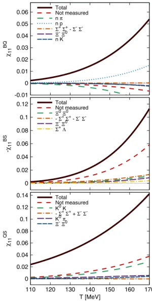
The result of this decomposition is that each of the correlators one can build between conserved charges is formed from the sum of many different particle-particle correlations. In particular, the sum of those correlators which entirely consist of observable species yields the measured part of a certain correlator, while its nonmeasured part consists of all other terms, which include at least one nonobservable species. In Fig.8the nondiagonal correla- tors are shown as a function of the temperature at vanishing chemical potential. The measured and nonmeasured con- tributions are shown with blue, dashed-dotted and red, dashed lines, respectively, while the full contribution is shown with a solid, thicker black line. Alongside the HRG

-0.03 -0.02 -0.01 0 0.01 0.02 0.03 0.04

χ11BQ

-0.05 0 0.05 0.1 0.15 0.2 0.25 0.3

- χ11BS

Total Measurable Not Measurable Lattice

-0.05 0 0.05 0.1 0.15 0.2 0.25 0.3

110 120 130 140 150 160 170 180 190 200 χ11QS

T [MeV]

FIG. 8. Second-order correlators of the conserved chargesB,Q, S. The total contribution, the measured and nonmeasured parts, evaluated in the HRG model, are shown in solid black, dotted- dashed blue and dashed red, respectively. The lattice results are shown as the magenta points.

model results, continuum extrapolated lattice results are shown as magenta points as introduced in Sec. II.

We notice that both the BQ and QS correlators are largely reproduced by the measured contribution (for the BQcorrelator, the measured portion even exceeds the full one, as the nonmeasured contribution is negative), while theBScorrelator is roughly split in half between measured and nonmeasured terms. This is because the former are unsurprisingly dominated by the net-proton and net-kaon contributions, respectively, which in this temperature regime form the bulk of particle production, together with the pions. The BScorrelator conversely receives its main contributions from strange baryons, which are almost equally split between measured and nonmeasured.

B. Breakdown of the measured and nonmeasured contributions

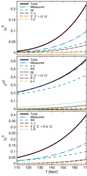
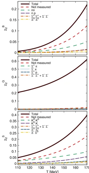
The decomposition in Eq.(26)allows one to break down the different contributions to any cross correlator, as well as the diagonal ones, entirely. In Figs.9and10, we show the breakdown of the measured portion of the single final state hadronic (self-) correlations to the nondiagonal and diago- nal correlators, respectively. Let us start from the non- diagonal case.

A few features can be readily noticed. First, in all cases only a handful of the most sizable contributions account for

0 0.01 0.02 0.03 0.04 0.05 0.06

χ11BQ

Total Measured ppp π Ξ^-Ξ^- + Ω^-Ω^- Λ πΛ K

0 0.02 0.04 0.06 0.08 0.1 0.12

-χ11BS

Total Measured ΛΛ

2 Ξ^- Ξ^- + 3 Ω^- Ω^- pKΛ K

Λ p

0 0.02 0.04 0.06 0.08 0.1 0.12 0.14

110 120 130 140 150 160 170

χ11QS

T [MeV]

Total Measured KK2 Ξ^- Ξ^- + 3 Ω^- Ω^- K π

Λπ Λ K

FIG. 9. Breakdown of the different final state hadronic con- tributions to the cross-correlators of the conserved chargesB,Q, Sat second order. The total contribution and the measured part are shown as solid black and dashed-dotted blue lines, respec- tively. The main single contributions from measured hadronic observables are shown with different colored dashed and dashed- dotted lines.

0 0.05 0.1 0.15 0.2

χ2B

Total Measured ppΛΛ Ξ^-Ξ^- + Ω^-Ω^- Λ p

0 0.1 0.2 0.3 0.4 0.5 0.6

χ2Q

Total Measured ππ KK pp Ξ^-Ξ^- + Ω^-Ω^- K π p π

0 0.05 0.1 0.15 0.2 0.25 0.3 0.35 0.4

110 120 130 140 150 160 170

χ2S

T [MeV]

Total Measured KKΛ Λ

4 Ξ^-Ξ^- + 9 Ω^-Ω^- Λ K

FIG. 10. Breakdown of the different final state hadronic contributions to the diagonal correlators of the conserved charges B,Q,Sat second order. The total contribution and the measured part are shown as solid black and dashed-dotted blue lines, respectively. The main single contributions from measured hadronic observables are shown with different colored dashed and dashed-dotted lines.

the measured portion of the corresponding observable. As stated above, theBQandQScorrelators are expected to be dominated by the contribution from net-proton and net- kaon self-correlations, respectively: indeed, in both cases the measured part almost entirely consists of these major contributions. Second, it is worth noticing how, with the only exception of the proton-pion correlator withinχ^BQ₁₁, all correlators between different species yield a very modest contribution. This is the case for the proton-kaon, kaon- pion, Lambda-pion and Lambda-kaon correlators in χ^BQ₁₁ and χ^QS₁₁, as well as theproton-kaon, Lambda-kaon and Lambda-proton correlators inχ^BS₁₁. In our setup, correlations between different particle species can only arise from the decay of heavier resonances. Whenever a resonanceRhas a nonzero probability to decay, after the whole decay cascade, both into stable speciesAandB, then a correlation arises betweenAandB. It can be seen from Eq.(27)that only when both probabilities in parentheses are nonzero can a nonzero correlation arise. For the same reason, correlations between different baryons arise, although no single decay mode with more that one baryon (or anti- baryon) is present in our decay list. In fact, if a state exists which has a finite probability to produce—after the whole decay cascade—both baryon A and baryon B, then a correlation between A and B is generated through Eq. (27). Finally, since both Ξ⁻ and Ω⁻ carry all three conserved charges, they contribute to all three correlators through their self-correlations, and their contribution is not negligible in all cases.

The case ofχ^BS₁₁ is slightly different, as the measured part is smaller than in the cases ofχ^QS₁₁ andχ^BQ₁₁ . This is due to the fact that there is no significant separation in mass between the lightest observable particle carrying both baryon number and strangeness—the Λ baryon—and the lightest of the nonmeasured ones—theΣ baryons. In fact, the contribu- tion from both chargedΣbaryons is comparable to the one from theΛ, which thus cannot play as big of a role as the proton and kaon in the other two correlators, as well as because of the previously mentioned fact that correlators of different species do not contribute significantly.

In the diagonal case, a similar picture appears. Theχ^Q₂ correlator is almost identical to its measured portion, dominated by the self-correlations of pions, kaons, and protons. The other two correlators have a similar situation to that ofχ^BS₁₁, with the measured part roughly amounting to half of the total. Again, the only non-negligible correlator between different species is the proton-pion correlator in χ^Q₂. We notice that in general, the leading single contribu- tion is not as close to the whole measured portion, as it was in the case of the cross-correlators. This aspect is important in the following, where we move to the analysis of ratios of correlators, and look for suitable proxies.

In Figs. 11 and 12 we show the breakdown of the nonmeasured portion of the final state hadronic (self-)

correlations, analogously to what we showed in Figs.9and 10for the measured portion. The situation in this case is slightly different from the previous one: it is generally more difficult to identify a leading contribution, with multiple terms yielding comparable results. In the case ofBQand QS, leading terms come with opposite signs, which further complicates the picture. The reasons for these features come from the fact that (i) the number of single contribu- tions that are not measured is much larger than that of the measured ones, hence it is less probable that few terms dramatically dominate; and (ii) in general, nonmeasured species are heavier than the measured ones, hence single contributions tend to be smaller. Obviously, exceptions to this are the neutron andK⁰. In fact, the diagonal correlators

-0.01 0 0.01 0.02 0.03 0.04 0.05 0.06

χ11BQ

Total Not measured n π n pΣ⁺ Σ⁺ - Σ^- Σ^- Ξ^- Ξ⁰ n K

0 0.02 0.04 0.06 0.08 0.1 0.12

-χ11BS

Total Not measured Ξ⁰ Ξ⁰ - Σ⁺ Σ⁺ - Σ^- Σ^- Ξ^- Ξ⁰ Σ⁺ Λ

0 0.02 0.04 0.06 0.08 0.1 0.12 0.14

110 120 130 140 150 160 170

χ11QS

T [MeV]

Total Not measured K⁰ K - Σ⁺ Σ⁺ + Σ^- Σ^- K⁰ π Ξ^- Ξ⁰

FIG. 11. Breakdown of the different final state hadronic contributions to the cross-correlators of the conserved charges B, Q, S at second order. The total contribution and the non- measured part are shown as solid black and dashed red lines, respectively. The main single contributions from nonmeasured hadronic observables are shown with different colored dashed and dashed-dotted lines.