Nucleon axial structure from lattice QCD

JHEP05(2020)126

Published for SISSA by Springer Received: January 10, 2020 Revised: March 13, 2020 Accepted: April 24, 2020 Published:May 26, 2020

Nucleon axial structure from lattice QCD

The RQCD collaboration

Gunnar S. Bali,^a,b Lorenzo Barca,^a Sara Collins,^a Michael Gruber,^a Marius L¨offler,^a Andreas Sch¨afer,^a Wolfgang S¨oldner,^a Philipp Wein,^a Simon Weish¨aupl^a and Thomas Wurm^a

aInstitut f¨ur Theoretische Physik, Universit¨at Regensburg, Universit¨atsstraße 31, D-93040 Regensburg, Germany

bDepartment of Theoretical Physics, Tata Institute of Fundamental Research, Homi Bhabha Road, Mumbai 400005, India

E-mail: gunnar.bali@ur.de,lorenzo1.barca@ur.de,sara.collins@ur.de, michael1.gruber@ur.de,marius.loeffler@ur.de,andreas.schaefer@ur.de, wolfgang.soeldner@ur.de,philipp.wein@ur.de,simon.weishaeupl@ur.de, thomas.wurm@ur.de

Abstract: We present a new analysis method that allows one to understand and model excited state contributions in observables that are dominated by a pion pole. We apply this method to extract axial and (induced) pseudoscalar nucleon isovector form factors, which satisfy the constraints due to the partial conservation of the axial current up to expected discretization effects. Effective field theory predicts that the leading contribution to the (induced) pseudoscalar form factor originates from an exchange of a virtual pion, and thus exhibits pion pole dominance. Using our new method, we can recover this behavior directly from lattice data. The numerical analysis is based on a large set of ensembles generated by the CLS effort, including physical pion masses, large volumes (with up to 96³×192 sites and Lmπ = 6.4), and lattice spacings down to 0.039 fm, which allows us to take all the relevant limits. We find that some observables are much more sensitive to the choice of parametrization of the form factors than others. On the one hand, the z-expansion leads to significantly smaller values for the axial dipole mass than the dipole ansatz (M_A^z-exp = 1.02(10) GeV versus M_A^dipole = 1.31(8) GeV). On the other hand, we find that the result for the induced pseudoscalar coupling at the muon capture point is almost independent of the choice of parametrization (g_P^{? z-exp} = 8.68(45) and g^?_P^dipole = 8.30(24)), and is in good agreement with both, chiral perturbation theory predictions and experimental measurement via ordinary muon capture. We also determine the axial coupling constantg_A. Keywords: Lattice QCD, Neutrino Physics, Nonperturbative Effects

ArXiv ePrint: 1911.13150

JHEP05(2020)126

Contents

1 Introduction 1

2 Correlation functions 3

2.1 Definitions 3

2.2 EFT-based analysis 5

2.3 Spectral decomposition 12

3 Data analysis 14

3.1 Lattice setup 14

3.2 Fits to the correlation functions 19

3.3 Excited state energies 26

4 Form factors 27

4.1 Approximate restoration of PCAC and PPD 27

4.2 Parametrization and extrapolation 28

4.2.1 Dipole ansatz 28

4.2.2 z-expansion 29

4.2.3 Consistency with PCAC in the continuum 30

4.2.4 Continuum, quark mass, and volume extrapolation 32

4.3 Results 34

4.4 Discussion 40

5 Summary 45

A Traces 48

B Fit ansatz for the subtracted currents 48

1 Introduction

The axial structure of the nucleon is relevant for the description of experiments that involve weak interactions. The most precisely known quantity in this context is the axial coupling constant g_A, which corresponds to the axial form factor at vanishing momentum trans- fer and can be determined experimentally from β decay (see refs. [1–3]; cf. also ref. [4]).

At finite momentum transfer Q², the axial and the induced pseudoscalar form factors are much less well known. They enter the description of exclusive pion electroproduction [5–8]

(e.g.,e⁻p→π⁻pν), (quasi-)elastic neutrino-nucleon scattering [9–12], radiative muon cap- ture [13–15], and ordinary muon capture [16–19]. Via weak muon capture in muonic hydrogen a combination of the Dirac, Pauli, axial, and induced pseudoscalar form factors

JHEP05(2020)126

can be measured, constraining the latter at the muon capture point [15,18–21]. The direct determination of the induced pseudoscalar coupling in refs. [18, 19] shows that, at small momentum transfer, the induced pseudoscalar form factor is indeed well approximated by a pion pole dominance (PPD) ansatz.

From the theoretical side, one can gain insight into the form factors through various techniques. At small momentum transfer, chiral perturbation theory (ChPT) yields valu- able low energy theorems [8,22–25] (motivating, e.g., the above mentioned PPD ansatz), while, at intermediate and large virtualities, the form factors can be determined (up to some systematic uncertainty of ∼15%) using light-cone sum rules [26,27]. Another interesting approach is the application of functional renormalization group methods [28].

In this work, we will use lattice QCD, which enables a determination of hadronic observables from first principles. Once all systematic uncertainties are under control, this method provides the cleanest and most direct access to hadron form factors. Many studies of nucleon couplings and form factors have been carried out in the past using a wide variety of lattice actions and analysis methods (see, e.g., refs. [29–63]). Recent studies of form factors at finite virtualities with data close to physical pion masses have faced two problems: first of all, it is difficult to reconcile the data with the partial conservation of the axial current (PCAC). Even though PCAC is approximately fulfilled on the correlation function level, the corresponding relation between the ground state form factors, which are extracted using a spectral decomposition, is broken to a much larger extent. Secondly, the PPD ansatz for the induced pseudoscalar form factor fails to describe the data at small momentum transfer and small pion masses, which is the domain where one would expect this ansatz to give the best approximation. In both cases an explanation in terms of finite lattice spacing effects is unlikely, since the violation of PCAC is largest at small virtualities and masses. For nice presentations of these problems see, e.g., refs. [55,58]. A prime suspect that may be responsible for both effects is a particularly large excited state contamination, albeit it was demonstrated in ref. [57] that the problem persist if one uses a traditional fit ansatz with up to three free excited states. In ref. [60] we have proposed a subtraction method that removes excited state contributions that violate the equations of motion for the nucleon. While this leads to a recovery of the PCAC relation on the form factor level, the PPD ansatz still remained strongly broken. While this is not impossible as such, the induced pseudoscalar charge at the muon capture point remained at variance with the experimental value [15,18–21].

A deeper insight into the excited state effects is possible using effective field theory (EFT). ChPT based analyses [64–66] (along the lines of refs. [67–70] using interpolating currents from ref. [71]) indicate that the subtraction method mentioned above does not remove all excited states and that the violation of the PPD ansatz is due to additional, large contributions from N π exited states that predominantly affect the induced pseu- doscalar and the pseudoscalar form factors. While an a posteriori subtraction of the effect performed in refs. [64,65] leads to satisfying results, such a procedure appears inadequate from the lattice QCD perspective as it introduces a dependence on ChPT input parame- ters and cannot be consistently combined with standard excited state fits. Moreover, when truncating the ChPT expansion for the interpolating currents at leading order (as, e.g., in

JHEP05(2020)126

refs. [64,65]) theN andN π overlap factors have the exact same dependence on the oper- ator smearing, which may not be justified in lattice simulations where spatially extended (smeared) nucleon interpolators with radii that are not very small compared to the inverse pion mass are employed.

The procedure advocated in this article makes use of the same effective field theory methods as refs. [64–66,72] in order to calculate the leading excited state contribution to the correlation function explicitly for all axial and pseudoscalar channels with less assumptions.

We will show that exploiting the EFT knowledge stabilizes excited state fits considerably and allows us to extract ground state form factors, which are found to obey both the PCAC relation on the form factor level and the PPD ansatz reasonably well. Recently an alternative analysis method has been proposed in ref. [73], which also allows an extraction of nucleon form factors that satisfy PCAC. We will discuss similarities and differences between our approach and this method in sections 3.3 and4.1.

This article is structured as follows. In section 2we will give a detailed description of the EFT calculation needed to determine the leading N π contribution to the correlation function and how it can be combined with the usual excited state analysis. The lattice setup and the employed ratios of correlation functions are detailed in section 3. Section 4 contains the results for the form factors (using both, dipole fits and the z-expansion) and includes an analysis of the PCAC relation as well as of the PPD ansatz. We also explore parametrizations that are consistent with PCAC in the continuum. In the latter case the continuum limit is under much better control. We summarize our findings in section 5.

2 Correlation functions

2.1 Definitions

In order to study hadron structure using lattice QCD one has to calculate two- and three- point correlation functions, where hadron states with matching quantum numbers are cre- ated by a suitable interpolating current ¯N at the source time t_src, and are destroyed by N at the sink time tsnk (here, we will always set tsrc = 0 and tsnk = t without loss of generality). In the case of three-point correlation functions one inserts a local current O at some insertion timeτ witht > τ >0 and, usually, one is interested in the ground state matrix element of this current insertion. The momenta can be fixed by appropriate Fourier transforms, in our case at the sink and the insertion, such that the initial state and final state momenta are p and p⁰, respectively:

C_2pt,P^p

+(t) =P₊^αβC_2pt,βα^p (t) =a³X

x

e^−ip·xP₊^αβhN^β(x, t) ¯N^α(0,0)i, (2.1) C_3pt,Γ^p0,p,O(t, τ) = Γ^αβC_3pt,βα^p0,p,O(t, τ)

=a⁶X

x,y

e^−ip0·x+i(p⁰−p)·yΓ^αβhN^β(x, t)O(y, τ) ¯N^α(0,0)i, (2.2) where C_2pt^p , C_3pt^p0,p,O, P+, and Γ are matrices in Dirac space with the corresponding spin indices α and β. The three-quark nucleon interpolating current is defined via the usual

JHEP05(2020)126

quark-diquark structure with the charge conjugation matrix C, N^α(x, t) = u(x, t)^TCγ5d(x, t)

u^α(x, t), (2.3)

where each quark is smeared separately in the spatial directions using Wuppertal smear- ing [74] on spatially APE-smoothed links [75]. Note that Minkowski scalar products and gamma matrix conventions are used throughout this work. At zero three-momentum P₊= (1+γ₀)/2 annihilates the leading negative parity contribution. For the analysis of the pseudoscalar and axialvector form factors we choose Γ to be P₊ⁱ =P₊γⁱγ5, i= 1,2,3. In order to relate the correlation functions to matrix elements, one inserts identity operators (corresponding to sums over all hadronic states) and uses the translational properties of the currents to carry out the Fourier transforms. When evaluating the result at large Eu- clidean times,t,τ, andt−τ, excited states are exponentially suppressed and the correlation functions can be approximated by the ground state contributions:

C_2pt,P^p

+(t)≈X

σ

P₊^αβh0|N^β|N_σ^pihN_σ^p|N¯^α|0ie^−Ept

2E_p , (2.4)

C_3pt,Γ^p0,p,O(t, τ)≈X

σ⁰,σ

Γ^αβh0|N^β|N_σ^p0⁰ihN_σ^p0⁰|O|N_σ^pihN_σ^p|N¯^α|0ie^{−Ep0(t−τ)}e^−Epτ 2E_p⁰2Ep

, (2.5)

where all currents are located at the origin and |N_σ^pi corresponds to a nucleon state with three-momentum p and spin-projection σ. The parity projected overlap matrix elements can be parametrized as

P_±^αβh0|N^β(0,0)|N_σ^pi=P_±^αβ q

Zp^±u^β_p,σ, (2.6)

whereu^βp,σ is a nucleon spinor and √

Z_p^±are momentum- and smearing-dependent overlap factors. For smeared currents√

Z_p⁺and√

Z_p⁻can differ from each other due to the explicit breaking of Lorentz invariance by the operator smearing, cf. refs. [76] and [77] for more details. Since in our analysis only positive parity projected overlap matrix elements occur, we define p

Z_p ≡ √

Z_p⁺. The form factor decomposition for the nucleon-nucleon matrix element of a generic current can be written as

hN_σ^p0⁰|O(0,0)|N_σ^pi= ¯u_p⁰_,σ⁰J[O]u_p,σ, (2.7) whereJ[O] is matrix valued and can be parametrized in terms of form factors, cf. eqs. (2.12) and (2.13) below. Using the spinor identity P

σup,σu¯p,σ=/p+m, wherem is the nucleon mass, one arrives at the ground state contribution

C_2pt^p (t)≈ Zp

2E_pe^−Ept(/p+m), (2.8)

C_3pt^p0,p,O(t, τ)≈

pZ_p⁰p Z_p

2E_p⁰2E_p e^{−Ep0(t−τ)}e^−Epτ(/p⁰+m)J[O](/p+m). (2.9) For the two-point function we can explicitly evaluate the trace with P₊ to find

C_2pt,P^p ₊(t)≈ Z_p 2Ep

e^−Epttr

P+(/p+m) =Zp

E_p+m Ep

e^−Ept. (2.10)

JHEP05(2020)126

For the three-point functions the trace with Γ depends on the current-specific decomposi- tion (2.7). In practice it turns out (in particular in case of the three-point functions) that, at Euclidean time distances t and τ with acceptable signal-to-noise ratio, not only the ground state contributes. In most cases this problem can be treated by taking into account generic excited state contributions in the fit functions (see section 2.3). However, there are situations in which the excited states constitute (at the available temporal distances) the dominant contribution. In the latter case the generic excited state parametrizations fail to describe the data appropriately and further physical insight into the excited state structure is needed, cf. section 2.2.

For the isovector pseudoscalar and axialvector currents used in this work,

P = ¯uγ₅u−dγ¯ ₅d , A_µ= ¯uγ_µγ₅u−dγ¯ _µγ₅d , (2.11) the explicit decompositions in terms of the pseudoscalar form factor, G_P(Q²), as well as the axial and induced pseudoscalar form factors, G_A(Q²) and G_P˜(Q²), are

J[P] =γ₅G_P(Q²), (2.12)

J[A_µ] =γ_µγ₅G_A(Q²) + qµ

2mγ₅G_P˜(Q²), (2.13) where q = p⁰ −p is the momentum transfer and Q² = −q² is the virtuality. The three form factors used above are not independent in the continuum theory, since the axial Ward identity yields ∂^µA_µ= 2i m`P known as partial conservation of the axialvector current (PCAC). Here m<sub>`</sub> is the light quark mass. On the lattice this relation can be broken by discretization effects. For the nucleon matrix elements it implies that

2i m_`hN_σ^p00|P|N_σ^pi=hN_σ^p00|∂^µA_µ|N_σ^pi+O(a²), (2.14) where we can safely ignore discretization effects linear in the lattice spacing a, since our analysis is fully order a improved, cf. section 3.1. Using the definitions (2.12) and (2.13) together with the equations of motion one can deduce the corresponding relation for the form factors (called PCACFF in ref. [60]):

m_`

mG_P(Q²) =G_A(Q²)− Q²

4m²G_P˜(Q²) +O(a²). (2.15) Eqs. (2.14) and (2.15) should both be satisfied, once the ground state matrix elements have been extracted reliably.

2.2 EFT-based analysis

Employing a theory where hadrons are the effective degrees of freedom (like baryon chiral perturbation theory) in order to elucidate the excited state structure in correlation func- tions is appealing, in particular if multi-hadron states with additional pions are the relevant excitations, see refs. [67–70,78]. In many cases, however, these contributions are relatively small and one can deal with them using standard methods like, e.g., source/sink-smearing and multi-exponential fits that allow for generic excited state contributions. As will be

JHEP05(2020)126

explained in detail in this section, the situation is different in the context of isovector axial and pseudoscalar form factors, where N π contributions can actually be a leading term from the EFT point of view due to pion pole dominance (PPD). Especially for small pion masses this effect outweighs the exponential suppression at the currently available source- sink distances due to the small energy gap.¹ In this situation multi-exponential fits with generic excited states become very unstable and usually fail to isolate the ground state contribution (see the discussions in refs. [55,57,58,60]).²

In refs. [65,66] nucleon three-point functions with axialvector and pseudoscalar current insertions have been analyzed using ChPT and compelling qualitative evidence has been presented that the violations of the PCAC and PPD relations are indeed caused by N π excited states. This is done as follows: first, one calculates the excited state contribution to the form factor using ChPT. The predicted, excited state contaminated form factor is found to agree quite well with recent data from the PACS collaboration [58], cf. refs. [66,72]. In a second step, one may attempt to correct the error by subtracting the calculated excited state contaminations a posteriori (see, e.g., refs. [64,65], where such a subtraction has been performed for the induced pseudoscalar form factor). While this method yields convincing qualitative results, there are some open questions and limitations that need to be addressed:

1. In general, the operator smearing can have a different effect on N and N π over- lap factors, which a leading order ChPT calculation does not allow for. There are heuristic arguments that this effect of the smearing should be negligible as long as the smearing radii rsm are much smaller than the Compton wavelength of the pion λπ ≈1.41 fm, cf. refs. [67,68,70,78]. This seems to contradict the observation that the operator smearing used in actual simulations has a strong impact on the signal of excited states. In refs. [38, 40] it has been found that smearing radii of roughly r_sm ∼0.5 fm maximize the ground state overlap. In the lattice analysis performed in this article, the optimized smearing radii are on some ensembles even larger (up to 0.8 fm, cf. table 2), and it is questionable whether a dependence on the smearing can be completely excluded for such smearing radii.³

2. So far, an a posteriori subtraction of the excited states has only been performed in combination with the ratio method on the lattice. It is unclear how one would avoid double counting, if one combines it with a standard excited state analysis, e.g., by using multi-exponential fits.

3. Estimating the systematic error tied to the ChPT based subtraction is challenging.

From a lattice QCD perspective the situation is in our opinion quite clear concerning point 2. If there is a large N π excited state contribution, then it should be taken into

1Note that, due to the exponential deterioration of the signal, one cannot expect the source-sink distances to become dramatically larger in future simulations.

2An alternative method has been proposed in ref. [73], which appears to resolve the ground state con- tribution in this situation. We will comment on this method in some detail in sections3.3and4.1.

3Note that our analysis in section3suggests that there is no strong suppression of the N π states due to the smearing and that the leading order ChPT approximation for the interpolating currents is actually quite good.

JHEP05(2020)126

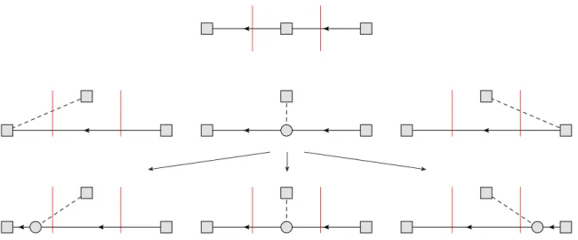
Figure 1. Feynman diagrams showing the most important (tree-level) contributions to the axial and pseudoscalar three-point functions. The squares correspond to explicitly inserted operators: the right and left ones correspond to smeared three-quark baryon interpolating currents at the source (at time 0) and the sink (at timet), respectively, while the ones in the middle depict a pseudoscalar or an axialvector operator insertion (at timeτ). The circles correspond to pion-nucleon interaction vertices, while the dashed and solid lines represent pion and nucleon propagators, respectively. The dotted red vertical lines indicate the sums over hadronic states one usually introduces to interpret correlation functions.

account explicitly in the multi-state fits to the correlation functions.⁴ In this approach point 1 can be addressed simultaneously by allowing for a smearing dependence of the N π coupling to the interpolating currents. Furthermore, we can avoid systematic uncertainties (point 3) by relaxing ChPT constraints. In the following, we will describe in detail how this can be achieved.

The first and second rows of figure 1 show the tree-level Feynman diagrams that contribute to the correlation functions. As discussed in ref. [65], these yield the most important contribution to the correlation function. The squares on the right and left depict the smeared source and sink currents, while the one in the middle corresponds to the inserted local quark bilinears (axialvector or pseudoscalar currents in our case).

The dashed and solid lines depict pion and nucleon propagators, while the circle stands for a pion-nucleon interaction vertex. The dotted red lines are for illustration only and indicate the identity operators (i.e., the sum over all hadronic states) that are usually inserted between source and current as well as between current and sink, cf. eq. (2.5). This elucidates that the diagram in the first row yields a contribution to the ground state, while the diagrams on the left- and right-hand sides in the second row give rise to a nucleon-pion excitation in the final and initial state, respectively. For the diagram in the middle of the

4One can also try to circumvent the problem entirely by either suppressing or subtracting the unwanted excited state contributions. In ref. [79] the pion pole contribution is suppressed by analyzing the matrix elements of currents with a Gaussian profile instead of local currents. Ref. [60] presents a method to subtract some of the excited state contributions.

JHEP05(2020)126

second row, however, the situation is not that simple, since the nucleon-pion interaction is not restricted to a specific time-slice. As a consequence, the diagram contributes to both the ground state and the excited states, as shown in the bottom row of figure 1.

This follows from an explicit calculation of the diagrams (see below). We emphasize that there is no one-to-one correspondence between the individual contributions in the spectral decomposition and the diagrams. For example, both the diagram in the first row and the diagram in the middle of the second row contribute to the ground state and, actually, an infinite number of diagrams will contribute to each state if one takes into account higher orders in ChPT (see ref. [65] for a list of one-loop diagrams). Finally, a single diagram can contribute to multiple states in the spectral decomposition, cf. the bottom row of figure 1.

We will exploit the fact that the pion pole contribution to the ground state automatically gives rise to an associated excited state.

Before addressing the details, let us note that the following calculation is in large parts already contained in refs. [65, 66], where also one-loop diagrams are taken into account.

Also the presentation in ref. [79] is based on similar considerations (cf. also ref. [80]).

However, we will present the result in a more general way (without using a particular spin projection or fixing initial and final state momenta to a predefined configuration) such that it can be used in a variety of simulation setups. The first ingredient we need in order to evaluate the diagrams in figure 1 are the corresponding Feynman rules. Here we follow the conventions of ref. [81], but adapt them to our choices for the currents (see eq. (2.11)) and convert them to position space. We work in two-flavor baryon ChPT here. However, since we only consider the nucleon sector and are only working at tree-level accuracy, a three-flavor calculation would give exactly the same result. Note that in this section all time variables are in Minkowski time and will be rotated to imaginary times only at the very end. The pion and nucleon propagators read

S_N(x) =i Z d⁴q

(2π)⁴e^−iq·x /q+m

q²−m²+i, (2.16)

S_π^ab(x) =δ^abSπ(x) =i Z d⁴q

(2π)⁴e^−iq·x δ^ab

q²−m²_π+i. (2.17)

For the vertices of the current insertions we have

A^µ =g_Aγ^µγ₅σ³, (2.18)

P = 0, (2.19)

A^µ =−2F_π∂^µδ^a3, (2.20)

P =−2iF_πBδ^a3, B≡ m²_π

2m_` , (2.21)

where we only take into account the leading contribution in the chiral counting⁵ and all derivatives are understood to act on the pion propagator. Here, F_π and g_A correspond to

5Note thatγ5 is counted as first order in baryon ChPT, while other elements of the Clifford algebra are counted as zeroth order, see, e.g., ref. [82]. This explains why the N N vertex of the pseudoscalar current vanishes at leading order.

JHEP05(2020)126

the pion decay constant and the axial coupling in the chiral limit, respectively, while B is the condensate parameter and σ^a are Pauli matrices. For the leading N π interaction vertex we have

=−i gA

2F_π∂γ/ 5σ^a. (2.22)

The vertices for local three-quark currents have been derived in ref. [71]. We adapt these to the smeared interpolating currents used here by allowing for momentum- and smearing- dependent couplings. With the nucleon isospinor ΨN, where Ψp= (1,0)^T and Ψn= (0,1)^T, the leading order vertices read

=p

Zp⁰Ψ¯N, =p

ZpΨN, (2.23)

=p Z˜_p,q i

2F_πΨ¯_Nγ₅σ^a, =p

Z˜_p⁰_,q i

2F_πγ₅σ^aΨ_N, (2.24) where one can actually assume Z_p =Z_p(p²) and Z_p,q = Z_p,q(p²,p·q,q²) up to lattice artifacts (obviously, the couplings will also depend on the masses, the smearing method and the smearing radii). We will use Z = Zp, Z⁰ = Z_p⁰, ˜Z = ˜Z_p⁰_,q, and ˜Z⁰ = ˜Zp,q as shorthand notations. In the following we always consider protons, i.e., ¯Ψ_pσ³Ψ_p = 1. We will not assume

pZ˜_p,q=p

Z_p⁰+ higher order, p

Z˜_p⁰_,q=p

Z_p+ higher order, (2.25) which should hold at least approximately for small smearing radii, as discussed above.

Instead, we will test the validity of this assumption by comparing it to our data, cf. figure5 in section3.2. We complete the setup with the definition of the following energies and four- momenta

E =p

p²+m², E⁰ =p

p⁰²+m², Eπ =p

(p⁰−p)²+m²_π, (2.26) p= E

p

!

, p⁰ = E⁰ p⁰

!

, q = E⁰−E p⁰−p

!

, r±= E_π

±(p⁰−p)

!

. (2.27)

We will now consider one example for each type of diagram in figure 1 with an axi- alvector current insertion, starting with the purely nucleonic diagram (in the first row of figure 1). Defining the four-vectors x = (t,x), y = (τ,y) and the energies E_i = q⁰_i, we obtain

√ Z⁰

√ Z

Z

d³x e^−ip0·x

Z

d³y e^−i(p−p0)·ySN(x−y)gAγ^µγ5SN(y) =

=−√ Z⁰√

Z Z dE₂

2π e^{−iE2(t−τ)} Z dE₁

2π e^−iE1τ(γ₀E₂−γ·p⁰+m)g_Aγ^µγ₅(γ₀E₁−γ·p+m) (E₂²−p⁰²−m²+i)(E₁²−p²−m²+i)

=

√ Z⁰√

Z

2E⁰2E e^{−iE0(t−τ)}e^−iEτ(/p⁰+m)g_Aγ^µγ₅(/p+m). (2.28) In the first step, one integrates over the positions which gives delta distributions in mo- mentum space, which in turn eliminate the integrals over the three-momenta from the

JHEP05(2020)126

propagators. Then, we close both integration contours in the lower half of the complex plane and use Cauchy’s residue theorem twice. Rotating to imaginary times (t→ −itand τ → −iτ) one obtains the axial part of eq. (2.9) to zeroth order accuracy in ChPT, exactly as expected.

Next, we consider the left diagram in the second row of figure 1, where the current insertion couples to a pion that directly connects to the sink, while the nucleon propagates directly from source to sink. We find

pZ˜⁰√ Z

Z

d³x e^−ip0·x

Z

d³y e^−i(p−p0)·y

i 2Fπ

γ₅

−2F_π ∂

∂yµ

S_π(x−y)S_N(x) =

=−p Z˜⁰√

Z Z dE₂

2π e^{−iE2(t−τ)} Z dE₁

2π e^−iE1t

E2

q

µ

E₂²−q²−m²_π+i

γ₅(γ₀E₁−γ·p+m) E₁²−p²−m²+i

= + pZ˜⁰√

Z

2E2E_π e^{−iEπ(t−τ)}e^−iEtr^µ₊γ₅(/p+m),

(2.29) where we have introduced the notation ^E_q²µ

, etc., to list the components of a 4-vector.

The pion carries the three-momentumq, while the nucleon propagates with momentump.

As in the first diagram, the integrals over the energies can be calculated independently.

The diagram yields anN π excitation in the final state with the energyE+Eπ. In general this will not be the excited state with the smallest possible energy. For the diagram where the pion propagates from the source to the insertion (cf. the right diagram in the second row of figure 1) one obtains, carrying out an analogous calculation,

−

√ Z⁰p

Z˜ 2E⁰2Eπ

e^−iE0te^−iEπτr^µ₋(/p⁰+m)γ5, (2.30) which yields an N π excitation in the initial state.

Finally, the diagram where the nucleon-pion interaction happens dynamically (the middle diagram in the second row of figure 1) gives

√ Z⁰

√ Z

Z

d³x e^−ip0·x

Z

d³y e^−i(p−p0)·y

Z d⁴z

×S_N(x−z)

−i g_A 2Fπ

γ_νγ₅ ∂

∂zν

−2F_π ∂

∂yµ

S_π(z−y)

S_N(z) =

=gA

√ Z⁰

√ Z

Z dE2

2π e^{−iE2(t−τ)} Z dE1

2π e^−iE1τ

×

E2−E1

q

µ E2−E1

q

ν

(E2−E1)²−q²−m²_π +i

(γ0E2−γ·p⁰+m)γνγ5(γ0E1−γ·p+m) (E₂²−p⁰²−m²+i)(E₁²−p²−m²+i) .

(2.31)

In this case, where the virtual pion has the three-momentumqand the energyE₂−E₁, the remaining integrations overE1 andE2 are not independent of each other. We will perform them consecutively starting with E1. Similarly to the procedure for the other diagrams, both integration contours can be closed in the lower half of the complex plane. There, the integrand has two single poles, which collapse to a double pole, ifE2 =E−Eπ. The latter case has to be treated separately. The result after the first integration is

g_A√ Z⁰√

Zi Z dE₂

2π f(E₂), (2.32)

JHEP05(2020)126

where, for E₂ 6=E−E_π,

f(E₂) =e^{−iE2(t−τ)}e^{−iEτ E2}_q^−E_{µ E2−E}

q

ν (γ0E2−γ·p⁰+m)γνγ5(/p+m)

2E((E2−E)²−E_π²+i)(E₂²−E⁰²+i) (2.33) +e^−iE2te^{−iEπτ −E}_q^πµ −Eπ

q

ν(γ₀E₂−γ·p⁰+m)γ_νγ₅(γ₀(E₂+E_π)−γ·p+m) 2Eπ(E₂²−E⁰²+i)((E2+Eπ)²−E²+i) . ForE₂=E−E_π, one can check thatf(E₂) is finite, which is the only relevant information since it means that there is no pole at this point when using the residue theorem for E2

later on. Thus, one finds thatf(E₂) has three poles in the lower half of the complex plane.

The first term in eq. (2.33) has two single poles, while the second term in eq. (2.33) has only one single pole. Its second, seeming pole is at E2 =E−Eπ, where eq. (2.33) is not evaluated. One obtains three contributions that correspond to the diagrams in the bottom row of figure 1:

−gA

√ Z⁰√

Z

2E⁰2E e^{−iE0(t−τ)}e^−iEτq^µq^ν(/p⁰+m)γ_νγ₅(/p+m) q²−m²_π

−g_A√ Z⁰√

Z 2E2Eπ

e^{−iEπ(t−τ)}e^−iEtr₊^µr₊^ν (/p+/r₊+m)γ_νγ₅(/p+m) (p+r+)²−m²

−gA

√ Z⁰√

Z

2E⁰2E_π e^−iE0te^−iEπτr^µ₋r^ν₋(/p⁰+m)γνγ5(/p⁰+/r₋+m) (p⁰+r−)²−m² ,

(2.34)

where we have written the result in terms of the four-vectors defined in eqs. (2.27). The first term yields a contribution to the ground state. It is responsible for the leading, pole dominant contribution to the induced pseudoscalar form factor. The second and the third term contribute to the same N π excitations in the final and initial states as those in eqs. (2.29) and (2.30), respectively.

This concludes our calculation of the tree-level diagrams shown in figure 1 for the axialvector current insertion. For the pseudoscalar current the calculation is analogous and we will not repeat it here. By matching the result obtained for the ground state with the usual form factor decompositions (using eq. (2.9) in combination with eqs. (2.12) and (2.13) after rotating to Euclidean times) one finds

G_A=g_A+ higher order, (2.35)

G_P˜ =g_A 4m²

Q²+m²_π + higher order, (2.36)

G_P =g_Am m_`

m²_π

Q²+m²_π + higher order. (2.37) We emphasize that we will not enforce these results for the ground state contribution. In eq. (2.35) this corresponds to augmenting the axial coupling in the chiral limit to the full axial form factor, which is justified at leading order accuracy. In the same spirit, we have already tacitly used the actual nucleon mass in the propagator instead of its chiral limit value, which is also correct to leading order accuracy in ChPT. It is consistent to perform the same replacementg_A7→G_Ain the complete calculation. (We will show that this choice

JHEP05(2020)126

is in much better agreement with the data at nonzeroQ², cf. section3.2and, in particular, figure5.) After doing so, eqs. (2.36) and (2.37) yield the PPD assumptions [83,84] for the (induced) pseudoscalar form factors, as expected.

It turns out to be convenient to define the ratios a=

pZ˜

√

Z , a⁰ =

pZ˜⁰

√

Z⁰ , (2.38)

wherea=a⁰ = 1 would correspond to the assumption that the smearing does not affect the overlap of the interpolating currents with theN π excited states (compared to the ground state). Note that in general a and a⁰ are functions of the momenta. Putting everything together and rotating to Euclidean time (t→ −itandτ → −iτ) we find

C_3pt^p0,p,Aµ = +

√ Z⁰√

Z

2E⁰2E e^{−E0(t−τ)}e^−Eτ(/p⁰+m)

G_Aγ^µγ₅+GP˜

q^µ 2mγ₅

(/p+m) (2.39)

−

√ Z⁰√

Z

2E2E_π e^{−(E+Eπ)(t−τ)}e^−Eτr₊^µ

b⁰γ5(/p+m) +GA

(/p+m)/r₊γ5(/p+m) (p+r₊)²−m²

+

√ Z⁰√

Z 2E⁰2Eπ

e^{−E0(t−τ)}e^{−(E0+Eπ)τ}r₋^µ

b(/p⁰+m)γ5−GA

(/p⁰+m)/r₋γ5(/p⁰+m) (p⁰+r−)²−m²

+. . . , C_3pt^p0,p,P = +

√ Z⁰√

Z

2E⁰2E e^{−E0(t−τ)}e^−Eτ(/p⁰+m)G_Pγ5(/p+m) (2.40)

−

√Z⁰√ Z 2E2Eπ

e^{−(E+Eπ)(t−τ)}e^−EτB

b⁰γ₅(/p+m) +G_A(/p+m)/r₊γ₅(/p+m) (p+r+)²−m²

−

√ Z⁰√

Z 2E⁰2Eπ

e^{−E0(t−τ)}e^{−(E0+Eπ)τ}B

b(/p⁰+m)γ₅−G_A(/p⁰+m)/r₋γ₅(/p⁰+m) (p⁰+r−)²−m²

+. . . , where

b=−a+G_A m²_π

(p⁰+r−)²−m², b⁰ =−a⁰+G_A m²_π

(p+r+)²−m² , (2.41) and the dots represent additional excited state contributions. These results can be used for all momentum configurations and with arbitrary spin projections. After taking the trace with the specific matrices P₊ⁱ that we use here, the result can be further simplified, see below. We emphasize that the leading, pole enhanced N π excited state contribution calculated here occurs either in the initial state or in the final state, but not in both simultaneously.

2.3 Spectral decomposition

In this section we will provide the explicit expressions for the correlation functions that are used in our analysis, including our parametrization of additional generic excited states.

For the latter we will assume that they occur with the same energies in both, two- and three-point functions. State-of-the-art lattice analyses of form factors take into account

JHEP05(2020)126

up to three excited states in the two-point and up to two excited states in the three- point functions, see, e.g., ref. [85]. Whether this is necessary depends on the available statistics and on the applied source/sink smearing. In our simulation a relatively large number of smearing steps was performed, leading to large smearing radii, cf. table 2. In this situation, we find it sufficient to add only one generic excited state to the two- and three-point correlators on top of the pion pole enhanced state that we have calculated in the last section. Including the additional generic excited state term, we obtain for the two-point function

C_2pt,P^p

+(t) =Zp

Ep+m Ep

e^−Ept 1 +Ape^−∆Ept

. (2.42)

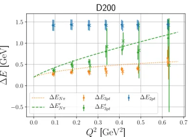
In the following we will abbreviate ∆E = ∆Ep and ∆E⁰ = ∆Ep⁰. Note that we do not assume any dispersion relation for the excited state energies, nor do we assume that these are single hadron states. Instead, we treat them as free fit parameters. We define the trace occurring in the ground state contribution to the three-point function as

B_Γ,O^p0,p = Tr

Γ(/p⁰+m)J[O](/p+m) . (2.43) The explicit results can be found in appendixA, together with the remaining traces needed to evaluate eqs. (2.39) and (2.40). For the three-point functions we obtain the parametriza- tion

C^p0,p,Aµ

3pt,P₊ⁱ =

√Z⁰√ Z

2E⁰2E e^{−E0(t−τ)}e^−Eτ (2.44)

×

B_P^p0,pi +,A^µ

1 +B₁₀e^{−∆E0(t−τ)}+B₀₁e^−∆Eτ +B₁₁e^{−∆E0(t−τ)}e^−∆Eτ +e^{−∆EN π0 (t−τ)}E⁰

Eπ

r^µ₊

c⁰pⁱ+d⁰qⁱ

+e^{−∆EN πτ} E Eπ

r₋^µ

c p⁰ⁱ+d qⁱ ,

C_3pt,P^p0,p,Pi +

=

√ Z⁰√

Z

2E⁰2E e^{−E0(t−τ)}e^−Eτ (2.45)

×

B_P^p0,pi +,P

1 +B₁₀e^{−∆E0(t−τ)}+B₀₁e^−∆Eτ+B₁₁e^{−∆E0(t−τ)}e^−∆Eτ +e^{−∆EN π0 (t−τ)}E⁰

Eπ

m²_π 2m`

c⁰pⁱ+d⁰qⁱ

−e^{−∆EN πτ} E Eπ

m²_π 2m`

c p⁰ⁱ+d qⁱ , where we have suppressed the dependence of the excited state parameters on the momenta, the spin-projection and the current insertion: Bij = Bij(p⁰,p,Γ,O). We have defined

∆E_{N π}=E_π + (E⁰−E), ∆E_{N π}⁰ =E_π−(E⁰−E) and c=−2b−4G_A mE_π+p⁰·r−

(p⁰+r−)²−m² , c⁰ =−2b⁰−4G_A mE_π+p·r₊

(p+r₊)²−m², (2.46) d=−G_A 4m(m+E⁰)

(p⁰+r−)²−m², d⁰ =G_A 4m(m+E)

(p+r₊)²−m² . (2.47) Equations (2.46) and (2.47) are only valid up to higher order corrections in ChPT. For instance, one could replaceG_A by (Q²+m²_π)G_P˜/(4m²) or by (Q²+m²_π)m_`G_P/(mm²_π) in

JHEP05(2020)126

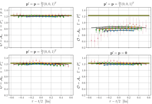
theN π excited state contributions (cf. eqs. (2.35), (2.36) and (2.37)) and the result would still be valid at leading order. From a plain vanilla ChPT power-counting point of view one could even replaceG_Abyg_A. Therefore, in anticipation of possible higher order corrections, we may relax the assumptions even further by usingc,c⁰,d, and d⁰ as free fit parameters, which reduces the ChPT input. This has the additional advantage, that it does not allow the excited state signal to have a direct influence on the result for the ground state form factors. Naturally, one has to pay for the increased number of fit parameters with a slightly larger statistical error for the ground state result — a small price considering that one gets rid of one source of systematic uncertainty. In section3.2 we will assess the validity of the ChPT predictions by comparing them to the results obtained from the fits. In particular we will be able to check whether the data is consistent with the parameter-free ChPT predic- tion fordand whether the direct coupling of the smeared three-quark interpolating currents to theN πstate differs from the leading order ChPT prediction calculated for local currents.

Note the elegance of the parametrization given in eqs. (2.44) and (2.45). Even after relaxing the conditions (2.46) and (2.47), it encodes the relative strength of theN πexcited state contribution in the different channels. The importance of this knowledge must not be underestimated. For instance, combining eq. (A.1) with eq. (2.44) one can see that any determination of the axial form factor using solely the A₁, A₂, and A₃ channels is not affected by these excited states at all.

Finally, let us note that for the kinematics we use in the numerical analysis, setting the final state momentum to zero, p⁰ = 0, such that p = −q (this setup is used in many lattice simulations), the parametrization becomes even simpler since one can replace c⁰pⁱ+d⁰qⁱ=e⁰qⁱ (withe⁰ =d⁰−c⁰) andc p⁰ⁱ+d qⁱ =dqⁱ. In this kinematic situation, theN π excited state energy corresponds toE_N(0)+E_π(−q) in the initial state, andE_N(p)+E_π(q) in the final state.

3 Data analysis

3.1 Lattice setup

In order to determine the axial and (induced) pseudoscalar form factors using the corre- lation functions described in section 2, we have analyzed a large set of lattice ensembles generated within the CLS effort [86].⁶ The ensembles have been generated using a tree- level Symanzik improved gauge action andN_f = 2 + 1 flavors of nonperturbatively ordera improved Wilson (clover) fermions. An efficient and stable hybrid Monte Carlo sampling is achieved by applying twisted-mass determinant reweighting [88], which avoids near-zero modes of the Wilson Dirac operator. The polynomial approximation of the strange quark determinant was corrected for by reweighting too, employing the method introduced in ref. [89]. The individual quarks in the nucleon interpolators at the source and the sink are Wuppertal-smeared [74], employing spatially APE-smoothed [75] gauge links. The

6The ensembles rqcd021, and rqcd030 have been generated using the BQCD code [87].

JHEP05(2020)126

β 3.40 3.46 3.55 3.70 3.85 a[fm] 0.086 0.076 0.064 0.050 0.039

Table 1. Lattice spacings a, corresponding to the five different inverse couplings β used in this study. The lattice spacings have been obtained by determining the Wilson flow time at the SU(3) symmetric point in lattice units t^∗₀/a² and equatingt^∗₀with the result µ^∗_ref= (8t^∗₀)^−1/2≈478 MeV of ref. [91].

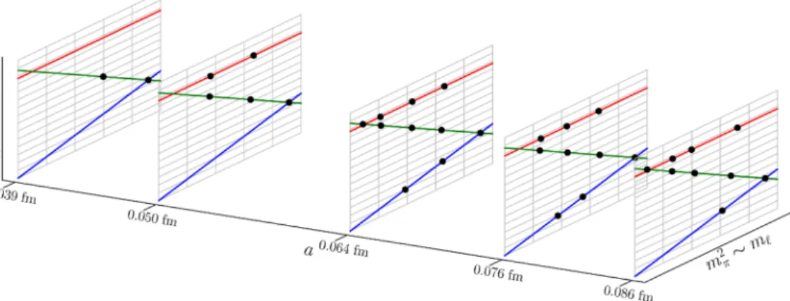
Figure 2. Schematic visualization of the analyzed CLS ensembles in the space spanned by the lattice spacing and quark masses. On the flavor symmetric plane (blue), where m_{`</sub> =m<sub>s</sub>, flavor multiplets of hadrons have degenerate masses (e.g., m<sup>2</sup><sub>K</sub> =m<sup>2</sup><sub>π</sub> and mN =mΣ=mΞ =mΛ). The green lines are defined to have physical average quadratic meson mass (2m<sup>2</sup><sub>K</sub>+m<sup>2</sup><sub>π</sub> = phys.). This corresponds to an approximately physical mean quark mass (2m<sub>`}+m_s≈phys.). The red lines are defined by 2m²_K−m²_π = phys. and indicate an almost physical strange quark mass (ms≈phys.).

Physical masses are reached at the intersections of green and red lines.

corresponding smearing radii r_sm are defined via r_sm² =

Ns/2−1

X

nx,ny,nz=−N_s/2

Ψ^†(na)n²a²Ψ(na),

Ns/2−1

X

nx,ny,nz=−N_s/2

Ψ^†(na)Ψ(na) = 1, (3.1) where Ψ is the normalized smearing function.

Some of the CLS ensembles (cf. table2for a full list of the ensembles used in this work) have been simulated employing very fine lattices down to a= 0.039 fm. For these lattices we avoid large autocorrelation times by using open boundary conditions in the time direc- tion [88,90]. The latter allow the topological charge to flow into and out of the simulation volume through the temporal boundaries and thus topological freezing is avoided. While employing open boundary conditions is crucial for fine lattice spacings, we use lattices with both open and periodic boundary conditions for the coarser spacings. In total we have five different lattice spacings ranging from a= 0.039 fm to a= 0.086 fm, see table1.

As illustrated in figure 2, the available ensembles have been generated along three different trajectories in the quark mass plane:⁷

7See also ref. [92]. In practice the ensembles do not always lie exactly on top of the green and red trajectories shown in figure2.