Fragmentation 3.0 Query Processing Architectures Fragmentation 3.0 Introduction

(1)

Christoph Lofi

Institut für Informationssysteme Technische Universität Braunschweig http://www.ifis.cs.tu-bs.de

Distributed Data Management

3.0 Query Processing

3.1 Basic Distributed Query Processing 3.2 Data Localization

3.3 Response Time Models

Distributed Data Management – Christoph Lofi – IfIS – TU Braunschweig 2

3.0 Introduction

•

There a 3 major architectures for DDBMS

–Share-Everything Architecture

•Nodes share main memory

•Suitably for tightly coupled high performance highly parallel DDBMS

•Weaknesses wrt. scalability and reliability –Shared-Disk Architecture

•Nodes have access to same secondary storage (usually SAN)

•Strengths wrt. complex data and transactions

•Common in enterprise level DDBMS –Share-Nothing Architecture

•Node share nothing and only communicate over network

•Common for web-age DDBMS and the cloud

•Strength wrt. scalability and elsaticity

Architectures

• Data has to be distributed across nodes

• Main concepts:

–Fragmentation: partition all data into smaller fragments / “chunks”

•How to fragment? How big should fragments be? What should fragments contain?

–Allocation: where should fragments be stored?

•Distribution and replication

•Where to put which fragment? Should fragments be replicated? If yes, how often and where?

Fragmentation

• In general, fragmentation and allocation are optimization problem which are closely depended on the actual application

–Focus on high availability?

–Focus on high degree of distribution?

–Focus on low communication costs and locality?

–Minimize or maximize geographic diversity?

–How complex is the data?

–Which queries are used how often?

• Many possibilities and decision!

Fragmentation

•

The task of DB query processing is to answer user

queries

–e.g. “How many students are at TU BS in 2009?”

•Answer: 14.100

•

However, some additional constraints must be satisfied

–Low response times –High query throughput –Efficient hardware usage –…

–Relational Databases 2!

3.0 Query Processing

(2)

• The generic workflow for centralized query processing involves multiple steps and components

3.0 Query Processing

Parser Query

Rewriter

Query Optimizer

Physical Optimizer

Query Execution

Query Result

Data Query Pre-Processing Meta Data

Catalog

• Query, Parser, and Naïve Query Plan

–Usually, the query is given by some higher-degree

declarative query language

•Most commonly, this is SQL

–The query is translated by parser into some internal representation

•Called naïve query plan

•This plan is usually described by an relational algebra operator tree

3.0 Query Processing

Parser Query

• Example:

–Database storing mythical creatures and heroes

•Creature(cid, cname, type); Hero(hid, hname)

•Fights(cid, hid, location, duration)

–“Return the name of all creatures which fought at the Gates of Acheron”

•SELECT cname FROM creature c, fights f WHERE c.cid=f.cid

AND location=“Gates Of Acheron”

3.0 Query Processing

• Example (cont.)

–Translate to relational algebra

•𝜋𝑐𝑛𝑎𝑚𝑒𝜎𝑙𝑜𝑐𝑎𝑡𝑖𝑜𝑛=^′𝐺𝑜𝐴^′∧𝑐𝑟𝑒𝑎𝑡𝑢𝑟𝑒.𝑐𝑖𝑑=𝑓𝑖𝑔ℎ𝑡𝑠.𝑐𝑖𝑑𝑐𝑟𝑒𝑎𝑡𝑢𝑟𝑒 × 𝑓𝑖𝑔ℎ𝑡𝑠

•In contrast to the SQL statement, the algebra statement already contains the required basic evaluation operators

3.0 Query Processing

• Example (cont.)

–Represent as operator tree

3.0 Query Processing

𝜋𝑐𝑛𝑎𝑚𝑒

𝜎_{𝑙𝑜𝑐𝑎𝑡𝑖𝑜𝑛=}′𝐺𝑜𝐴^′ ∧ 𝑐𝑟𝑒𝑎𝑡𝑢𝑟𝑒.𝑐𝑖𝑑=𝑓𝑖𝑔ℎ𝑡𝑠.𝑐𝑖𝑑

×

𝐶𝑟𝑒𝑎𝑡𝑢𝑟𝑒𝑠 𝐹𝑖𝑔ℎ𝑡𝑠

• After the naïve query plan is found, the query rewriter performs simple transformations

–Simple optimizations which are always beneficial regardless of the system state (Algebraic Query Rewriting)

• Mostly, cleanup operations are performed

• Elimination of redundant predicates

• Simplification of expressions

• Normalization

• Unnesting of subqueries and views

• etc.

–System state

• Size of tables

• Existence or type of indexes

• Speed of physical operations

• etc.

3.0 Query Processing

Query Rewriter

Meta Data Catalog

(3)

• The most effort in query preprocessing is spent on query optimization

–Algebraic Optimization

•Find a better relational algebra operation tree

•Heuristic query optimization

•Cost-based query optimization

•Statistical query optimization –Physical Optimization

•Find suitable algorithms for implementing the operations

3.0 Query Processing

Query Optimizer

Physical Optimizer

Meta Data Catalog

• Heuristic query optimization –Use simple heuristics which usually lead

to better performance

–Basic Credo: Not the optimal plan is needed, but the really crappy plans have to be avoided!

–Heuristics

•Break Selections

–Complex selection criteria should be broken into multiple parts

•Push Projection and Push Selection

–Cheap selections and projections should be performed as early as possible to reduce intermediate result size

•Force Joins

–In most cases, using a join is much cheaper than using a Cartesian product and a selection

3.0 Query Processing

• Example (cont.)

–Perform algebraic optimization heuristics

•Push selection & Projection

•Force Join

3.0 Query Processing

𝜋𝑐𝑛𝑎𝑚𝑒

𝜎𝑙𝑜𝑐𝑎𝑡𝑖𝑜𝑛=^′𝐺𝑜𝐴^′

⋈

𝐶𝑟𝑒𝑎𝑡𝑢𝑟𝑒𝑠

𝐹𝑖𝑔ℎ𝑡𝑠

𝜋𝑐𝑖𝑑, 𝑐𝑛𝑎𝑚𝑒 𝜋𝑐𝑖𝑑

•

Most non-distributed RDBMS rely strongly on cost-

based optimizations

–Aim for better optimized plan which respect system and data characteristics

•Especially, join order optimization is a challenging problem –Idea

•Establish a cost model for various operations

•Enumerate all query plans

•Pick best query plan

–Usually, dynamic programming techniques are used to keep computational effort manageable

3.0 Query Processing

• Algebraic optimization results in an optimized query plan which is still represented by

relational algebra

–How is this plan finally executed?

•> Physical Optimization

–There are multiple algorithms for implementing a given relational algebra operation

•Join: Block-Nested-Loop join? Hash-join? Merge-Join? etc.

•Select: Scan? Index-lookup? Ad-hoc index generation &

lookup? etc.

•…

3.0 Query Processing

• Physical optimization translates the query plan

into an execution plan

–Which algorithms will be used on which data and indexes?

•Physical Relational Algebra

–For each standard algebra operation, several physical implementations are offered

•Should pipelining (iterator model) be used? How?

–Physical and algebraic optimization are often tightly interleaved

•Most physical optimization also relies on cost-models

•Idea: perform cost-based optimization algorithm “in one sweep”

for algebraic, join order, and physical optimization

3.0 Query Processing

(4)

• Example (cont.)

3.0 Query Processing

Filter all but cname

Index Key Lookup:

fights.location=“GoA”

Index Nested Loop Join

Table 𝐶𝑟𝑒𝑎𝑡𝑢𝑟𝑒𝑠 Primary Index

Of Creatures

• In general, centralized non-distributed query processing is a well understood problem

–Current problems

•Designing effective and efficient cost models

•Eliciting meaningful statistics for use in cost models

•Allow for database self-tuning

3.0 Query Processing

• Distributed query processing (DQP) shares many properties of centralized query processing

–Basically, the same problem…

–But: objectives and constraints are different!

• Objectives for centralized query processing

– Minimize number of disk accesses!

– Minimize computational time

3.1 Basic DQP

• Objectives for distributed query processing are usually less clear…

–Minimize resource consumption?

–Minimize response time?

–Maximize throughput?

• Additionally, costs are more difficult to predict

–Hard to elicit meaningful statistics on network and

remote node properties

•Also, high variance in costs

3.1 Basic DQP

• Additional cost factors, constraints, and problems must be respected

–Extension of physical relational algebra

•Sending and receiving data –Data localization problems

•Which node holds the required data?

–Deal with replication and caching –Network models

–Response-time models

–Data and structural heterogeneity

•Think federated database…

3.1 Basic DQP

•

Often, static enumeration optimizations do are difficult in distributed setting

–More difficult than non-distributed optimization

•More and conflicting optimization goals

•Unpredictability of costs

•More costs factors and constraints

• Quality-of-Service agreements (QoS)

–Thus, most successful queries optimization techniques are adaptive

•Query is optimized on-the-fly using current, directly measured information of the system’s behavior and workload –Don’t target for the best plan,

but for a good plan

3.1 Basic DQP

(5)

•

Example distributed query processing:

–“Find the creatures involved in fights being decided in exactly one minute”

•𝜋_{𝑐𝑛𝑎𝑚𝑒}𝜎𝑑𝑢𝑟𝑎𝑡𝑖𝑜𝑛=1𝑚𝑖𝑛𝑐𝑟𝑒𝑎𝑡𝑢𝑟𝑒 ⋈ 𝑓𝑖𝑔ℎ𝑡𝑠 –Problem:

•Relations are fragmented and distributed across five nodes

•The creature relation uses primary horizontal partitioning by creature type

–One fragment of the relation is located at node 1, the other on node 2;

no replication

•The fights relation uses derived horizontal partitioning –One fragment on node 3, one on node 4; no replication

•Query originates from node 5

3.1 Basic DQP

N1

N2 N3

N4 N5

𝐶𝑟𝑒𝑎𝑡𝑢𝑟𝑒𝑠1

𝐶𝑟𝑒𝑎𝑡𝑢𝑟𝑒𝑠2 𝐹𝑖𝑔ℎ𝑡𝑠1

𝐹𝑖𝑔ℎ𝑡𝑠2 Query

• Cost model and relation statistics

–Accessing a tuple (tupacc) costs 1 unit –Transferring a tuple (tuptrans) costs 10 units –There are 400 creatures and 1000 fights

•20 fights are one minute

•All tuples are uniformly distributed –i.e. node 3 and 4 contain 10 short-fight-tuples each

–There are local indexes on attribute “duration”

•Direct tuple access possible on a local sites, no scanning –All nodes may directly communicate with each other

3.1 Basic DQP

N1

N2 N3

N4 N5

𝐶𝑟𝑒𝑎𝑡𝑢𝑟𝑒𝑠1

𝐶𝑟𝑒𝑎𝑡𝑢𝑟𝑒𝑠2 𝐹𝑖𝑔ℎ𝑡𝑠1

𝐹𝑖𝑔ℎ𝑡𝑠2 Query

𝜋𝑐𝑛𝑎𝑚𝑒𝜎𝑑𝑢𝑟𝑎𝑡𝑖𝑜𝑛=1𝑚𝑖𝑛𝑐𝑟𝑒𝑎𝑡𝑢𝑟𝑒 ⋈ 𝑓𝑖𝑔ℎ𝑡𝑠

200 tuples 200 tuples

500 tuples 10 matches 500 tuples

10 matches

• Two simple distributed query plans

–Version A: Transfer all data to node 5

3.1 Basic DQP

𝜋𝑐𝑛𝑎𝑚𝑒 (𝐶𝑟𝑒𝑎𝑡𝑢𝑟𝑒1∪ 𝐶𝑟𝑒𝑎𝑡𝑢𝑟𝑒2) ⋈ (𝜎𝑑𝑢𝑟𝑎𝑡𝑖𝑜𝑛=1𝑚𝑖𝑛𝐹𝑖𝑔ℎ𝑡𝑠1∪ 𝐹𝑖𝑔ℎ𝑡𝑠2) Node 5

Receive 𝐶𝑟𝑒𝑎𝑡𝑢𝑟𝑒1 Receive 𝐶𝑟𝑒𝑎𝑡𝑢𝑟𝑒1 Receive 𝐹𝑖𝑔ℎ𝑡𝑠1 Receive 𝐹𝑖𝑔ℎ𝑡𝑠2

Send 𝐶𝑟𝑒𝑎𝑡𝑢𝑟𝑒1

Node 1

Node 2 Node 4

Send 𝐹𝑖𝑔ℎ𝑡𝑠2

Node 3 Send 𝐹𝑖𝑔ℎ𝑡𝑠1

–Version B: ship intermediate results

3.1 Basic DQP

𝜋𝑐𝑛𝑎𝑚𝑒 (𝐶𝑟𝑒𝑎𝑡𝑢𝑟𝑒1∗∪ 𝐶𝑟𝑒𝑎𝑡𝑢𝑟𝑒2∗) Node 5

𝐶𝑟𝑒𝑎𝑡𝑢𝑟𝑒1∗

Receive 𝐹𝑖𝑔ℎ𝑡𝑠1∗ Send 𝐹𝑖𝑔ℎ𝑡𝑠1∗

Node 3 ^{𝐶𝑟𝑒𝑎𝑡𝑢𝑟𝑒}¹^{⋈𝐹𝑖𝑔ℎ𝑡𝑠}¹^∗ Node 1

𝜎𝑑𝑢𝑟𝑎𝑡𝑖𝑜𝑛=1𝑚𝑖𝑛𝐹𝑖𝑔ℎ𝑡𝑠1

Send 𝐶𝑟𝑒𝑎𝑡𝑢𝑟𝑒1∗

Node 4

𝐶𝑟𝑒𝑎𝑡𝑢𝑟𝑒2⋈𝐹𝑖𝑔ℎ𝑡𝑠₂∗

Node 2

𝜎𝑑𝑢𝑟𝑎𝑡𝑖𝑜𝑛=1𝑚𝑖𝑛𝐹𝑖𝑔ℎ𝑡𝑠2 Send 𝐶𝑟𝑒𝑎𝑡𝑢𝑟𝑒2∗

(6)

• Costs A: 23.000 Units

3.1 Basic DQP

𝜋𝑐𝑛𝑎𝑚𝑒 (𝐶𝑟𝑒𝑎𝑡𝑢𝑟𝑒1∪ 𝐶𝑟𝑒𝑎𝑡𝑢𝑟𝑒2) ⋈ (𝜎𝑑𝑢𝑟𝑎𝑡𝑖𝑜𝑛=1𝑚𝑖𝑛𝐹𝑖𝑔ℎ𝑡𝑠1∪ 𝐹𝑖𝑔ℎ𝑡𝑠2) Node 5

Receive 𝐶𝑟𝑒𝑎𝑡𝑢𝑟𝑒1 Receive 𝐶𝑟𝑒𝑎𝑡𝑢𝑟𝑒1 Receive 𝐹𝑖𝑔ℎ𝑡𝑠1 Receive 𝐹𝑖𝑔ℎ𝑡𝑠2

Node 1

Node 2 Node 4

Send 𝐹𝑖𝑔ℎ𝑡𝑠2

Node 3 Send 𝐹𝑖𝑔ℎ𝑡𝑠1 200*tuptrans

=2.000

200*tuptrans

=2.000

500*tuptrans

=5.000

500*tuptrans

=5.000 1.000*tupacc

=1.000 (selection w/o index) 400*20*tupacc

=8.000 (BNL join)

tupacc=1; tuptrans=10

• Cost B: 460 Units

3.1 Basic DQP

𝜋𝑐𝑛𝑎𝑚𝑒 (𝐶𝑟𝑒𝑎𝑡𝑢𝑟𝑒1∗∪ 𝐶𝑟𝑒𝑎𝑡𝑢𝑟𝑒2∗) Node 5

Node 3 ^{𝐶𝑟𝑒𝑎𝑡𝑢𝑟𝑒}¹^{⋈𝐹𝑖𝑔ℎ𝑡𝑠}¹^∗ Node 1

𝜎𝑑𝑢𝑟𝑎𝑡𝑖𝑜𝑛=1𝑚𝑖𝑛𝐹𝑖𝑔ℎ𝑡𝑠1

Send 𝐶𝑟𝑒𝑎𝑡𝑢𝑟𝑒1∗

Node 4

𝐶𝑟𝑒𝑎𝑡𝑢𝑟𝑒2⋈𝐹𝑖𝑔ℎ𝑡𝑠₂^∗

Node 2

𝜎𝑑𝑢𝑟𝑎𝑡𝑖𝑜𝑛=1𝑚𝑖𝑛𝐹𝑖𝑔ℎ𝑡𝑠2 Send 𝐶𝑟𝑒𝑎𝑡𝑢𝑟𝑒2∗

10*tupacc

=10 10*tuptrans

=100

10*tuptrans

=100

10*tupacc

=10 20*tupacc

=20 20*tupacc

=20 10*tuptrans

=100

10*tuptrans

=100 tupacc=1; tuptrans=10

• For performing any query optimization meta data is necessary

–Meta data is stored in the catalog

–The catalog of a DDBMS especially has to store information on data distribution

• Typical catalog contents

–Database schema

•Definitions of tables, views, UDFs & UDTs, constraints, keys,

etc.

3.1 Basic DQP

–Partitioning schema

•Information on how the schema is partitioned and how tables can be reconstructed

–Allocation schema

•Information on where which fragment can be found

•Thus, also contains information on replication of fragments –Network information

•Information on node connections

•Connection information (network model) –Additional physical information

•Information on indexes, data statistics (basic statistics, histograms, etc.), hardware resources (processing & storage ), etc.

3.1 Basic DQP

•

Central problem in DDBMS:

Where and how should the catalog be stored?

–Simple solution: store at a central node

–For slow networks, it beneficial to replicate the catalog across many / all nodes

•Assumption: catalog is small and does not change often –Also, caching is a viable solution

•Replicate only needed parts of a central catalog, anticipate potential inconsistencies

–In rare cases, the catalog may grow very large and may change often

•Catalog has to be fragmented and allocated

•New meta problem: where to find which catalog fragment?

3.1 Basic DQP

•

What should be optimized when and where?

–We assume that most applications use canned queries

•i.e. prepared and parameterized SQL statements

• Full compile time-optimization

–Similar to centralized DBs, the full query execution plan is computed at compile time

–Pro:

•Queries can be directly executed –Con:

•Complex to model

•Many information unknown or too expensive to gather (collect statistics on all nodes?)

•Statistics outdated

–Especially, machine load and network properties are very volatile

3.1 Basic DQP

(7)

• Fully dynamic optimization

–Every query is optimized individually at runtime –Heavily relies on heuristics, learning algorithms, and

luck –Pro

•Might produce very good plans

•Uses current network state

•Also usable for ad-hoc queries –Con

•Might be very unpredictable

•Complex algorithms and heuristics

3.1 Basic DQP

• Semi-dynamic and hierarchical approaches

–Most DDBMS optimizers use semi-dynamic or

hierarchical optimization techniques (or both) –Semi-dynamic

•Pre-optimize the query

•During query execution, test if execution follows the plan –e.g. if tuples/fragments are delivered in time, if network has

predicted properties, etc.

•If execution shows severe plan deviations, compute a new query plan for all missing parts

3.1 Basic DQP

• Hierarchical Approaches

–Plans are created in multiple stages –Global-Local Plans

•Global query optimizer creates a global query plan –i.e. focus on data transfer: which intermediate results are to be

computed by which node, how should intermediate results be shipped, etc.

•Local query optimizers create local query plans –Decide on query plan layout, algorithms, indexes, etc. to deliver the

requested intermediate result

3.1 Basic DQP

–Two-Step-Plans

•During compile time, only stable parts of the plan are computed

–Join order, join methods, access paths, etc.

•During query execution, all missing plan elements are added

–Node selection, transfer policies, …

•Both steps can be performed using traditional query optimization techniques

–Plan enumeration with dynamic programming

–Complexity is manageable as each optimization problem is much easier than a full optimization

–During runtime optimization, fresh statistics are available

3.1 Basic DQP

•

The first problem in distributed query processing is

data localization

–Problem: query transparency is needed

•User queries the global schema

•However, the relations of global schema are fragmented and distributed

– Assumption

•Fragmentation is given by partitioning rules –Selection predicates for horizontal partitioning –Attribute projection for vertical partitioning

•Each fragment is allocated only at one node –No replication

•Fragmentation rules and location of the fragments is stored in catalog

3.2 Data Localization

• Base Idea:

–Query Rewriter is modified such that each query to global schema is replaced by a query on the distributed schema

•i.e. each reference to a global relation is replaced by a localization program which reconstructs the table –If the localization program reconstructs the full

relation, this is called a generic query –Often, the full relation is not necessary and by

inspecting the query, simplifications can be performed

•Reduction techniques for the localization program

3.2 Data Localization

(8)

• Example:

–Relation 𝐶𝑟𝑒𝑎𝑡𝑢𝑟𝑒 = (𝑐𝑖𝑑, 𝑐𝑛𝑎𝑚𝑒, 𝑡𝑦𝑝𝑒) –Primary partitioning by id

•𝐶𝑟𝑡1= 𝜎𝑐𝑖𝑑≤100𝐶𝑟𝑒𝑎𝑡𝑢𝑟𝑒

•𝐶𝑟𝑡2= 𝜎100<𝑐𝑖𝑑<200𝐶𝑟𝑒𝑎𝑡𝑢𝑟𝑒

•𝐶𝑟𝑡3= 𝜎𝑐𝑖𝑑≥200𝐶𝑟𝑒𝑎𝑡𝑢𝑟𝑒

–Allocate each fragment to its own node

•𝐶𝑟𝑡1 to node 1, …

–A generic localization program for 𝐶𝑟𝑒𝑎𝑡𝑢𝑟𝑒 is given by

•𝐶𝑟𝑒𝑎𝑡𝑢𝑟𝑒 = 𝐶𝑟𝑡1∪ 𝐶𝑟𝑡2∪ 𝐶𝑟𝑡3

3.2 Data Localization

• Global queries can now easily be transformed to generic queries by replacing table references

–SELECT * FROM creatures WHERE cid = 9

•Send and receive operations are implicitly assumed

3.2 Data Localization

𝜎𝑐𝑖𝑑=9 𝐶𝑟𝑒𝑎𝑡𝑢𝑟𝑒𝑠 Global Query

∪ 𝐶𝑟𝑡1 𝐶𝑟𝑡2 𝐶𝑟𝑡3 Localization P. for Creatures

𝜎𝑐𝑖𝑑=9

∪ 𝐶𝑟𝑡1 𝐶𝑟𝑡2 𝐶𝑟𝑡3

Generic Query

• Often, when using generic queries, unnecessary fragments are transferred and accessed

–We know the partitioning rules, so it is clear that the requested tuple is in fragment 𝐶𝑟𝑡₁

–Use this knowledge to reduce the query

3.2 Data Localization

𝜎𝑐𝑖𝑑=9 𝐶𝑟𝑡1 Reduced Query

•

In general, the reduction rule for primary

horizontal partitioning can be stated as

–Given fragments of 𝑅 as 𝐹𝑅= 𝑅1, … , 𝑅𝑛 with 𝑅𝑗= 𝜎𝑃_𝑗(𝑅)

–Reduction Rule 1:

•All fragments 𝑹𝒋 for which 𝝈𝒑𝒔𝑹𝒋 = ∅ can be omitted from localization program

–𝒑𝒔 is the query selection predicate

–e.g. in previous example, 𝑐𝑖𝑑 = 9 contradicts 100 < 𝑐𝑖𝑑 < 200

•𝜎𝑝𝑠 𝑅𝑗 = ∅ ⇐ ∀𝑥 ∈ 𝑅: ¬(𝑝𝑠𝑥 ∧ 𝑝𝑗(𝑥))

•“The selection with the query predicate 𝑝𝑠 on the fragment 𝑅𝑗

will be empty if 𝑝_𝑠 contradicts the partitioning predicate 𝑝_𝑗 of 𝑅_𝑗”

–i.e. 𝑝𝑠 and 𝑝𝑗 are never true at the same time for all tuples in 𝑅𝑗

3.2 Data Localization

• Join Reductions

–Similar reductions can be performed with queries involving a join and relations partitioned along the join attributes

–Base Idea: Larger joins are replaced by multiple partial joins of fragments

• 𝑹𝟏∪ 𝑹𝟐 ⋈ 𝑺 ≡ 𝑹𝟏⋈ 𝑺 ∪ (𝑹𝟐⋈ 𝑺)

•Which might or might not be a good idea depending on the data or system

•Reduction: Eliminate all those unioned fragments from evaluation which will return an empty result

3.2 Data Localization

• i.e.: join according to the join graph

–Join graph usually not known (full join graph assumed)

•Discovering the non-empty partial joins will construct join graph

3.2 Data Localization

Fragments of R Fragments of S

R1R2R3R4 S1S2S3S4

(9)

•

We hope for

–…many partial joins which will definitely produce empty results and may be omitted

•This is not true if partitioning conditions are suboptimal –…many joins on small relations have lower resource

costs than one large join

•Also only true if “sensible” partitioning conditions used

•Not always true, depends on used join algorithm and data distributions; still a good heuristic

–…smaller joins may be executed in parallel

•Again, this is also not always a good thing

•May potentially decrease response time…

–Response time cost models!

•…but may also increase communication costs

3.2 Data Localization

• Example:

–𝐶𝑟𝑒𝑎𝑡𝑢𝑟𝑒 = (𝑐𝑖𝑑, 𝑐𝑛𝑎𝑚𝑒, 𝑡𝑦𝑝𝑒)

•𝐶𝑟𝑡2= 𝜎100<𝑐𝑖𝑑<200𝐶𝑟𝑒𝑎𝑡𝑢𝑟𝑒

•𝐶𝑟𝑡3= 𝜎𝑐𝑖𝑑≥200𝐶𝑟𝑒𝑎𝑡𝑢𝑟𝑒

–𝐹𝑖𝑔ℎ𝑡𝑠 = (𝑐𝑖𝑑, ℎ𝑖𝑑, 𝑙𝑜𝑐𝑎𝑡𝑖𝑜𝑛, 𝑑𝑢𝑟𝑎𝑡𝑖𝑜𝑛)

•𝐹𝑔1= 𝜎𝑐𝑖𝑑≤200𝐹𝑖𝑔ℎ𝑡𝑠

•𝐹𝑔2= 𝜎𝑐𝑖𝑑>200𝐹𝑖𝑔ℎ𝑡𝑠

–SELECT * FROM creature c, fight f WHERE c.cid=f.cid

3.2 Data Localization

⋈ 𝐶𝑟𝑒𝑎𝑡𝑢𝑟𝑒𝑠

Global Query

𝐹𝑖𝑔ℎ𝑡𝑠

⋈

𝐶𝑟𝑡1

Generic Query

∪

𝐶𝑟𝑡2 𝐶𝑟𝑡3 𝐹𝑔1

∪ 𝐹𝑔2

∪

𝐶𝑟𝑡1

Reduced Query

⋈ 𝐹𝑔1 𝐶𝑟𝑡2

⋈ 𝐶𝑟𝑡3

⋈ 𝐹𝑔2

• By splitting the joins, six fragment joins are created

• 3 of those fragment joins are empty

• e.g. 𝐶𝑟𝑡1⋈ 𝐹𝑔2= ∅

• 𝐶𝑟𝑡1contains tuples with cid≤100

• 𝐹𝑔2 contains tuples with cid>200

• Formally

–Join Fragmentation

• 𝑅1∪ 𝑅2 ⋈ 𝑆 ≡ 𝑅1⋈ 𝑆 ∪ (𝑅2⋈ 𝑆) –Reduction Rule 2:

𝑅_𝑖⋈ 𝑅_𝑗= ∅ ⇐ ∀𝑥 ∈ 𝑅_𝑖, 𝑦 ∈ 𝑅_𝑗: ¬(𝑝_𝑖 𝑥 ∧ 𝑝_𝑗(𝑦))

•“The join of the fragments 𝑅𝑗 and 𝑅𝑖 will be empty if their respective partition predicates (on the join attribute) contradict.”

–i.e. there is no tuple combination 𝑥 and 𝑦 such that both partitioning predicates are fulfilled at the same time

•Empty join fragments may be reduced

3.2 Data Localization

• Obviously, the easiest join reduction case follows from derived horizontal fragmentation

–For each fragment of the first relation, there is exactly one matching fragment of the second relation

•The reduced query will always be more beneficial than the generic query due to small number of fragment joins –Derived horizontal fragmentation is especially effective

to represent one-to-many relationships

•Many-to-many relationships are only possible if tuples are replicated

–No fragment disjointness!

3.2 Data Localization

• Example:

–𝐶𝑟𝑒𝑎𝑡𝑢𝑟𝑒 = (𝑐𝑖𝑑, 𝑐𝑛𝑎𝑚𝑒, 𝑡𝑦𝑝𝑒)

•…

–𝐹𝑖𝑔ℎ𝑡𝑠 = (𝑐𝑖𝑑, ℎ𝑖𝑑, 𝑙𝑜𝑐𝑎𝑡𝑖𝑜𝑛, 𝑑𝑢𝑟𝑎𝑡𝑖𝑜𝑛)

•𝐹𝑔1= 𝐹𝑖𝑔ℎ𝑡𝑠 ⋉ 𝐶𝑟𝑒𝑎𝑡𝑢𝑟𝑒

•…

–SELECT * FROM creature c, fight f WHERE c.cid=f.cid

3.2 Data Localization

∪

𝐶𝑟𝑡1

Reduced Query

⋈ 𝐹𝑔1 𝐶𝑟𝑡2

⋈ 𝐶𝑟𝑡3

⋈ 𝐹𝑔2 𝐹𝑔3

(10)

• Reduction for vertical fragmentation is very similar

–Localization program for 𝑅 is usually of the form

•𝑅 = 𝑅1⋈ 𝑅2

–When reducing generic vertically fragmented queries, avoid joining in fragments containing useless attributes –Example:

•𝐶𝑟𝑒𝑎𝑡𝑢𝑟𝑒 = (𝑐𝑖𝑑, 𝑐𝑛𝑎𝑚𝑒, 𝑡𝑦𝑝𝑒) is fragmented to 𝐶𝑟𝑒𝑎𝑡𝑢𝑟𝑒1= (𝑐𝑖𝑑, 𝑐𝑛𝑎𝑚𝑒) and 𝐶𝑟𝑒𝑎𝑡𝑢𝑟𝑒2= (𝑐𝑖𝑑, 𝑡𝑦𝑝𝑒)

•For the query SELECT cname FROM creature WHERE cid=9, no access to 𝐶𝑟𝑒𝑎𝑡𝑢𝑟𝑒2 is necessary

3.2 Data Localization

• Reducing Queries w. Hybrid Fragmentation

–Localization program for 𝑅 combines joins and

unions

•e.g. 𝑅 = (𝑅1∪ 𝑅2) ⋈ 𝑅3

–General guidelines are

•Remove empty relations generated by contradicting selections on horizontal fragments

–Relations containing useless tuples

•Remove useless relations generated by vertical fragments –Relations containing unused attributes

•Break and distribute joins, eliminate empty fragment joins –Fragment joins with guaranteed empty results

3.2 Data Localization

• Previously, we computed reduced queries from global queries

• However, where should the query be executed?

–Assumption: only two nodes involved

•i.e. client-server setting

•Server stores data, query originates on client –Query shipping

•Common approach for centralized DBMS

•Send query to the server node

•Server computes the query result and ships result back

3.2 Data Localization

–Data Shipping

•Query remains at the client

•Server ships all required data to the client

•Client computes result

3.2 Data Localization

Server Client

σ

B

⋈ receive

Query Shipping Data Shipping

Client

⋈

Server

A B

σ A

σ σ

send

receive receive

send send

• Hybrid Shipping

–Partially send query to server –Execute some query parts at the server, send intermediate results to client

–Execute remaining query at the client

3.2 Data Localization

Hybrid Shipping

59

Client

⋈

Server

A B

receive receive

send send

σ σ

• Of course, these simple models can be extended to multiple nodes

–Query optimizer has to decide which parts of the query have to be shipped to which node

•Cost model!

–In heavily replicated scenarios, clever hybrid shipping can effectively be used for load balancing

•Move expensive computations to lightly loaded nodes

•Avoid expensive communications

3.2 Data Localization

(11)

•

“Classic” DB cost models focus on

total resource consumption of a query

–Leads to good results for heavy computational load and slow network connections

•If query saves resources, many queries can be executed in parallel on different machines

–However, queries can also be optimized for short response times

•“Waste” some resources to get query results earlier

•Take advantage of lightly loaded machines and fast connections

•Utilize intra-query parallelism

–Parallelize one query instead of multiple queries

3.3 Response Time Models

• Response time models are needed!

–“When does the first result tuple arrive?”

–“When have all tuples arrived?”

• Example

–Assume relations or fragments A, B, C, and D –All relations/fragments are available on all nodes

•Full replication

–Compute 𝐴 ⋈ 𝐵 ⋈ 𝐶 ⋈ 𝐷 –Assumptions

•Each join costs 20 time units (TU)

•Transferring an intermediate result costs 10 TU

•Accessing relations is free

•Each node has one computation thread

3.3 Response Time Models

• Two plans:

–Plan 1: Execute all operations on one node

•Total costs: 60

–Plan 2: Join on different nodes, ship results

•Total costs: 80

3.3 Response Time Models

Node 1

A

⋈ ⋈

⋈

B C D

Node 1

A

⋈ ⋈

B C D

Send Send

Node 2 Node 3

Receive Receive

⋈ Plan 1

Plan 2

• With respect to total costs, plan 1 is better

• Example (cont.)

–But: Plan 2 is better wrt. to response time as operations can be carried out in parallel

3.3 Response Time Models

Time Plan 2

Plan 1 𝐴 ⋈ 𝐵 𝐶 ⋈ 𝐷

𝐴𝐵 ⋈ 𝐶𝐷 𝐶 ⋈ 𝐷 𝑇𝑋

𝑇𝑋

𝐴𝐵 ⋈ 𝐶𝐷

𝐴 ⋈ 𝐵

0 10 20 30 40 50 60

• Response Time

–Two types of response times

•First Tuple & Full Result Response Time

• Computing response times

–Sequential execution parts

•Full response time is sum of all computation times of all used operations

–Multiple parallel threads

•Maximal costs of all parallel sequences

3.3 Response Time Models

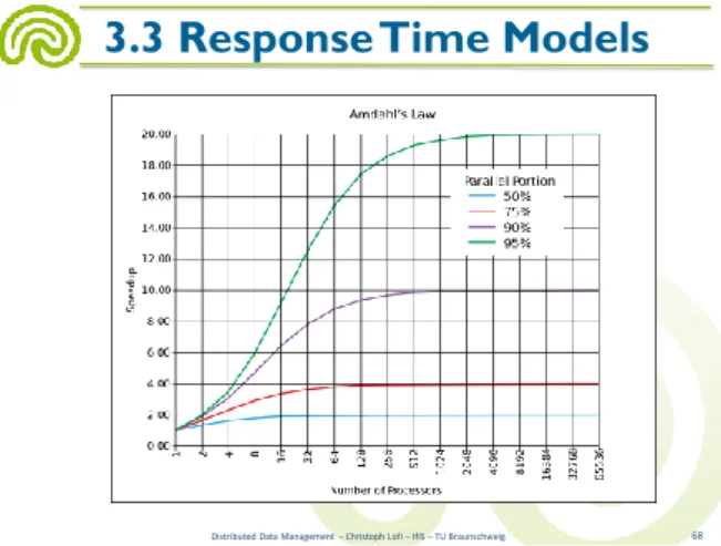
• Considerations:

–How much speedup is possible due to parallelism?

•Or: “Does kill-it-with-iron” work for parallel problems?

–Performance speed-up of algorithms is limited by Amdahl’s Law

•Gene Amdahl, 1968

•Algorithms are composed of parallel and sequential parts

•Sequential code fragments severely limit potential speedup of parallelism!

3.3 Response Time Models

(12)

–Possible maximal speed-up:

•𝑚𝑎𝑥𝑠𝑝𝑒𝑒𝑑𝑢𝑝 ≤_{1+𝑠∗ 𝑝−1}^𝑝

•𝑝 is number of parallel threads

•𝑠 is percentage of single-threaded code – e.g. if 10% of an algorithm is sequential, the

maximum speed up regardless of parallelism is 10x –For maximal efficient parallel systems, all sequential

bottlenecks have to be identified and eliminated!

3.3 Response Time Models

• Good First Tuple Response benefits from queries executed in a pipelined fashion

–Not pipelined:

•Each operation is fully completed and a intermediate result is created

•Next operation reads intermediate result and is then fully completed

–Reading and writing of intermediate results costs resources!

–Pipelined

•Operations do not create intermediate results

•Each finished tuple is fed directly into the next operation

•Tuples “flow” through the operations

3.3 Response Time Models

• Usually, the tuple flow is controlled by iterator interfaces implemented by each operation

–“Next tuple” command

–If execution speed of operations in the pipeline differ, tuples are either cached or the pipeline blocks

• Some operations are more suitable than others for pipelining

–Good: scan, select, project, union, … –Tricky: join, intersect, …

–Very Hard: sort

3.3 Response Time Models

•

Simple pipeline example:

–Tablescan, Selection, Projection

•1000 tuples are scanned, selectivity is 0.1 –Costs:

•Accessing one tuple during tablescan: 2 TU (time unit)

•Selecting (testing) one tuple: 1 TU

•Projecting one tuple: 1 TU

3.3 Response Time Models

FInal Projection

IR1 Table Scan

IR2 Selection

Table Scan Selection Projection

Pipeline

Final time event

2 First tuple in IR1 2000 All tuples in IR1 2001 First tuple in IR2 3000 All tuples in IR2 3001 First tuple in Final 3100 All tuples in Final

time event 2 First tuple finished

tablescan 3 First tuple finished

selection (if selected…) 4 First tuple in Final 3098 Last tuple finished

tablescan 3099 Last tuple finished

selection 3100 All tuples in Final Pipelined

Non-Pipelined

•

Consider following example:

–Joining two table subsets

•Non-pipelined BNL join

•Both pipelines work in parallel –Costs:

•1.000 tuples are scanned in each pipeline, selectivity 0.1

•Joining 100 ⋈100 tuples: 10,000 TU (1 TU per tuple combination) –Response time (non-pipelined BNL)

•The first tuple can arrive at the end of any pipeline after 4 TU –Stored in intermediate result

•All tuples have arrived at the end of the pipelines after 3,100 TU

•Final result will be available after 13,100 TU –No benefit from pipelining wrt. response time –First tuple arrives at 3100 ≪ 𝑡 ≤ 13100

3.3 Response Time Models

Table Scan Selection Projection

BNL Join

Pipeline

(13)

• The suboptimal result of the previous example is due to the unpipelined join

–Most traditional join algorithms are unsuitable for pipelining

•Pipelining is not usually necessary feature in a strict single thread environment

–Join is fed by two input pipelines –Only one pipeline can be executed at a time –Thus, at least one intermediate result has to be created –Join may be performed single / semi-pipelined

•In parallel / distributed DBs, fully pipelined joins are beneficial

3.3 Response Time Models

• Single-Pipelined-Hash-Join –One of the “classic” join algorithms –Base idea 𝑨 ⋈ 𝑩

•One input relation is read from an intermediate result (B), the other is pipelined though the join operation (A)

•All tuples of B are stored in a hash table –Hash function is used on the join attribute

–i.e. all tuples showing the same value for the join attribute are in one bucket

»Careful: hash collisions! Tuple with different joint attribute value might end up in the same bucket!

•Every incoming tuple a (via pipeline) of A is hashed by join attributed

•Compare a to each tuple in the respective B bucket –Return those tuples which show matching join attributes

3.3 Response Time Models

• Double-Pipelined-Hash-Join –Dynamically build a hashtable for A

and B each

•Memory intensive!

–Process tuples on arrival

•Cache tuples if necessary

•Balance between A and B tuples for better performance

•Rely on statistics for a good A:B ratio

–If a new A tuple a arrives

•Insert a into the A-table

•Check in the B table if there are join partners for a

•If yes, return all matching AB tuples –If a new B tuple arrives, process it

analogously

3.3 Response Time Models

Hash Tuple 17 A1, A2

31 A3

Hash Tuple

29 B1

A B

A Hash B Hash

Input Feeds AB Output Feed

𝑨 ⋈ 𝑩

31 B2

3.3 Response Time Models

Hash Tuple 17 A1, A2 31 A3

Hash Tuple 29 B1 31 B2

A B

A Hash B Hash

Input Feeds AB Output Feed

𝑨 ⋈ 𝑩

31 B2

• B(31,B2) arrives

• Insert into B Hash

• Find matching A tuples

• Find A3

• Assume that A3 matches B2…

• Put AB(A3, B2) into output feed

•

In pipelines, tuples just “flow” through the operations

–No problem with that in one processing unit…

–But how do tuples flow to other nodes?

•

Sending each tuple individually may be very

ineffective

–Communication costs:

•Setting up transfer & opening communication channel

•Composing message

•Transmitting message: header information & payload –Most protocols impose a minimum message size & larger headers –Tuplesize ≪ Minimal Message Size

•Receiving & decoding message

•Closing channel

3.3 Response Time Models

• Idea: Minimize Communication Overhead by Tuple Blocking

–Do not send single tuples, but larger blocks containing multiple tuples

•“Burst-Transmission”

•Pipeline-Iterators have to be able to cache packets

•Block size should be at least the packet size of the underlying network protocol

–Often, larger packets are more beneficial –….more cost factors for the model

3.3 Response Time Models

(14)

• Additional constraints and cost factors compared to “classic” query optimization

–Network costs, network model, shipping policies –Fragmentation & allocation schemes

–Different optimization goals

•Response time vs. resource consumption

• Basic techniques try to prune unnecessary accesses

–Generic query reductions

Distributed Query Processing

• This lecture only covers very basic techniques

–In general, distributed query processing is a very

complex problem

–Many and new optimization algorithms are researched

•Adaptive and learning optimization

•Eddies for dynamic join processing

•Fully dynamic optimization

•…

• Recommended literature

–Donald Kossmann: “The state of the Art in Distributed Query Processing”, ACM Computing Surveys, Dec. 2000

Distributed Query Processing

• Distributed Transaction Management

–Transaction Synchronization

–Distributed Two-Phase Commits –Byzantine Agreements