Upwelling and isolation in oxygen-depleted anticyclonic modewater eddies and implications for nitrate cycling

1

Upwelling and isolation in oxygen-depleted anticyclonic modewater eddies and implications for nitrate cycling

Johannes Karstensen¹, Florian Schütte¹, Alice Pietri², Gerd Krahmann¹, Björn Fiedler¹, Damian Grundle¹, Helena Hauss¹, Arne Körtzinger^1,3, Carolin R. Löscher¹, Pierre Testor², Nuno Viera⁴, Martin Visbeck^1,3

5

1GEOMAR, Helmholtz Zentrum für Ozeanforschung Kiel, Düsternbrooker Weg 20, 24105 Kiel, Germany

2LOCEAN, UMPC; Paris, France

3Kiel University, Kiel Germany

4Instituto Nacional de Desenvolvimento das Pescas (INDP), Cova de Inglesa, Mindelo, São Vicente, Cabo Verde Correspondence to: Johannes Karstensen (jkarstensen@geomar.de)

10

Abstract. The physical (temperature, salinity, velocity) and biogeochemical (oxygen, nitrate) structure of an oxygen depleted coherent, baroclinic, anticyclonic mode-water eddy (ACME) is investigated using high-resolution autonomous glider and ship data. A distinct core with a diameter of about 70 km is found in the eddy, extending from about 60 to 200 m depth and. The core is occupied by fresh and cold water with low oxygen and high nitrate concentrations, and bordered by local maxima in buoyancy 15

frequency. Velocity and property gradient sections show vertical layering at the flanks and underneath the eddy characteristic for vertical propagation (to several hundred-meters depth) of near inertial internal waves (NIW) and confirmed by direct current measurements. A narrow region exists at the outer edge of the eddy where NIW can propagate downward. NIW phase speed and mean flow are of similar magnitude and critical layer formation is expected to occur. An asymmetry in the NIW pattern is 20

seen that possible relates to the large-scale Ekman transport interacting with ACME dynamics.

NIW/mean flow induced mixing occurs close to the euphotic zone/mixed layer and upward nutrient flux is expected and supported by the observations. Combing high resolution nitrate (NO3-) data with the apparent oxygen utilization (AOU) reveals AOU:NO3- ratios of 16 which are much higher than in the surrounding waters (8.1). A maximum NO3- deficit of 4 to 6 µmol kg^-1 is estimated for the low oxygen 25

core. Denitrification would be a possible explanation. This study provides evidence that the recycling of NO3-, extracted from the eddy core and replenished into the core via the particle export, may quantitatively be more important. In this case, the particulate phase is of keys importance in decoupling the nitrogen from the oxygen cycling.

Introduction 30

Eddies are associated with a wide spectrum of dynamical processes from the mesoscale (order of several 10 to 100 km) to the submesoscale (order of 10 meters to less than 1 km). The interaction of these processes creates transport patterns in and around eddies that provoke intense biogeochemical and biological feedback (Levy et al. 2012, Chelton et al. 2011a). At the ocean surface, the eddy rotation generates a sea level anomaly (SLA) pattern that allow for their remote detection (Chelton et al. 2011a).

35

2

But also in other surface parameters, such as seas surface temperature (SST) or chlorophyll-a fluoresence, eddies show anomalies that allow deriving their statistics (Chelton et al. 2011b; Gaube et al. 2015). Utilizing satellite data large/global scale analysis of eddy-generated anomalies has been conducted (Chaigneau et al. 2009, Chelton et al. 2011a, Gaube et al. 2015). More recently the vertical structure of mesoscale eddies have been studied on regional (Chaigneau et al. 2011) and global scale 5

(Zhang et al. 2013) combining eddy surface detection with concurrent, but opportunistic, in-situ profile data (e.g. Argo floats). These studies differentiate, based on the SLA being either positive or negative, cyclonically rotating and anti-cyclonically rotating eddies.

However, when vertical stratification is considered, a third group of mesoscale eddies emerges that combine the downward displacement of isopycnals towards the eddy centre, as observed in “normal”

10

anticyclonic eddies (AE), with the upward displacement of isopycnals, characterizing cyclonic eddies (CE). Such “hybrid eddies” are called anticyclonic mode-water eddies (ACME) or intra-thermocline eddies (McWilliams 1985, D’Asaro 1988, Kostianoy and Belkin 1989, Thomas 2008), because the depth interval between upward and downward displaced isopycnals creates a volume of rather homogenous properties, sometimes called “mode” water. A recent study (Schütte et al. 2015) 15

investigated the occurrence of these three different types of mesoscale eddies (CE, AE, and ACME) in the eastern tropical North Atlantic, combining in-situ profile data with satellite SLA and SST data. The authors found that ACME in the tropical eastern North Atlantic are characterized by a cold SST anomaly (in contrast to AEs that show a warm SST anomaly), which allowed a statistical assessment of ACME in the tropical eastern North Atlantic based on satellite data alonse. Schütte et al. (2015) 20

estimated that about 9% of all eddies (20% of all anticyclones) in the eastern tropical North Atlantic are ACME.

More than a decade ago a dedicated observational program was carried out to survey eddies in western North Atlantic (Sargasso Sea) in order to better understand the physical-biogeochemical interactions.

The surveys revealed that ACME showed particularly intense deep chlorophyll-a layers that aligned 25

with a maximum concentrations of diatoms and maximum productivity (McGillicuddy et al. 2007). The high productivity was linked to a conceptual model that explains the intense vertical fluxes of nutrients within ACME with an Ekman divergence generated from the horizontal gradient in wind stress across an ACME (McGuillicuddy et al. 2007; going back to a work from Dewar and Flierl, 1987). The concept itself was questioned (Mahadevan et al. 2008) and high-resolution ocean model simulations, comparing 30

runs with or without eddy-wind interaction, reproduced only a marginal impact on ocean productivity (but a strong impact on physics; Eden and Dietze 2009). However, from a tracer release experiment within an ACME the magnitude of the vertical flux was found to be of the magnitude as expected from simple eddy-wind induced Ekman pumping estimates (order of meters per day; Ledwell et al. 2008).

3

A measure for the importance of local rotational effect relative to the Earth rotation is given by the Rossby number defined as 𝑅𝑜=_!^!, and where 𝜁=^!"_!"−^!"_!" is the vertical vorticity (𝑈,𝑉 are zonal and meridional velocity) and 𝑓 the planetary vorticity. Planetary flows have small Ro say up to ~0.2, while local rotational effects gain importance with Ro approaching 1. Mesoscale eddies often have Ro close to 1 indicating that, for example, the geostrophic approximation does not hold locally. Anticyclonic 5

rotating eddies (AE and ACME) have negative relative vorticity (𝜁<0) and modify 𝑓 into an effective planetary vorticity (𝑓!""=𝑓+^!_!) (Kunze 1985, Lee and Niller 1998). This local reduction in 𝑓 has for example implications for the propagation of internal waves that occur at frequencies in the range of the local buoyancy frequency (N) and 𝑓. For AEs, the local reduction of 𝑓 leads to a trapping of internal waves of near inertial frequencies (NIW) and downward energy propagation inside of AEs (Kunze 10

1985, Gregg et al. 1986, Lee and Niller 1998, Koszalka et al. 2010, Joyce et al. 2013, Alford et al.

2016). Depending on the vertical distribution of N the downward NIW propagation can generate an amplification of the wave energy and eventually part of that energy is dissipated by critical layer absorption which in turn results in intense vertical mixing (Kunze 1985, Kunze et al. 1995, Whitt and Thomas 2013).

15

The anticyclonic rotation of ACME also reduces f but, in contrast to AE, a local N maximum at their upper boundary characterizes the ACME. This N maximum creates a “cap” and complicates NIW vertical propagation. Lee and Niller (1998) considered an ACME stratification in a model study on near inertial internal wave propagation, mimicking the stratification of a “California subsurface warm core eddy”, and found the accumulation of energy below the eddy. A recent study (Sheen et al. 2015) 20

reported on hydrography, dissipation measurements, and current observations across an ACME observed at 2000 m depth in the Antarctic Circumpolar Current. The study found enhanced diapycnal mixing at the periphery of this particular ACME. Applying a ray tracing method to a stability profile from outside and from inside of the eddy Sheen et al. showed that, depending on their propagation direction relative to the background shear, the modelled internal waves either encounter a critical layer 25

above and below the eddy or are reflected at the eddy core.

A number of studies analysed NIW interaction with Mediterranean Outflow lenses in the North Atlantic (“Meddies”, Armi and Zenk 1984), which are deep ACME (mode below 1000m). Krahmann et al.

(2008) reported observations of enhanced NIW energy at the rim of a Meddie. For Meddies signatures of layering at the eddy periphery have often been observed and related to the interaction of NIW with 30

the baroclinic shear of the rotating lens, ultimately driving dissipation (Hua et al. 2013). The dissipation is often associated with Kelvin-Helmholtz instabilities (e.g. Kunze et al. 1995) but other mixing processes, such as double-diffusion may play a role too. In particular layering, produced by internal wave shear and strain, has been also reported to enhance double diffusive fluxes (St Laurent and

4

Schmitt 1999), at least in regions that are already characterized by salt finger-favourable stratification (Kunze 1995).

Levy et al. (2012) summarized the submesoscale upwelling at fronts in general, not specifically for mesoscale eddies, and the impact on oceanic productivity. Vertical property flux of nutrients into the euphotic zone plays a key role in the productivity scenarios and can be either by advection or by 5

mixing. Regardless of the mechanism for vertical transport, mesoscale eddies have been found to be

“retention regions” (d’Ovidio et al. 2013) and the upwelling of properties into the mixed layer, either inside or at the periphery of mesoscale eddies, is trapped in the eddy where it can be utilized efficiently.

Recently, ACME with very low oxygen concentrations in their cores where observed in the tropical eastern North Atlantic (Karstensen et al. 2015). The generation of the low oxygen concentrations was 10

linked to high productivity in the euphotic zone of the eddy and the subsequent remineralisation of the sinking organic matter, a process that requires a vertical fluxes of nutrients to supply the productivity in the euphotic zone. However, the eddy core were found to be highly isolated against surrounding waters and weak transport and mixing activity in and around the core was expected. As such it is surprising that the isolated core can exist in parallel to the enhanced vertical flux, and that suggested that the 15

processes responsible for the separation must act on small spatial scales. In this paper we further investigate the transport processes associated with a low oxygen ACME making use of high-resolution underwater glider and ship data. This paper is part of a series of publications that report on different genomic, biological and biogeochemical aspects of low oxygen ACME in the eastern tropical North Atlantic (Löscher et al. 2015, Hauss et al. 2016, Fiedler et al. 2016, Schütte et al. 2016).

20

2 Data and Methods

Targeted eddy surveys are logistically challenging. Eddy locations can be identified using real-time satellite SLA data. To further differentiate a positive SLA (indicative for anticyclonic rotation) into either an AE or an ACME the SST anomaly across the eddy was inspected, because ACME in the eastern tropical North Atlantic show a cold SST anomaly (Schütte et al. 2015, Schütte et al. 2016). For 25

further evidence, but purely opportunistic, Argo profile data were inspected to detect anomalously low temperature/salinity signatures, indicative of low oxygen ACME in the region (Karstensen et al. 2015, Schütte et al 2016). In late December 2013 a candidate eddy was identified through this mechanisms and in late January 2014 a pre-survey was initiated, making use of autonomous gliders. After confirmation that the candidate eddy was indeed a low oxygen ACME, two ship surveys (ISL, M105;

30

Fiedler et al. 2016) and further glider surveys followed.

5 2.1 Glider survey

Data from the glider IFM13 (1st deployment) and Glider IFM12 (2nd deployment) were used in this study (Fig. 1). IFM12 surveyed temperature, salinity, and oxygen to a depth of 500 m while IFM13 surveyed the same properties down to 700 m. Both glider measured chlorophyll-a fluorescence and turbidity to 200 m depth. In addition to the standard sensors IFM13 was also equipped with a nitrate 5

sensor that sampled to 700 m depth. IFM13 surveyed one full eddy section from April 3-7, 2014 (Fig. 1). For IFM12 we combined data from February 3-5 and from February 7-10, 2014 because, due to technical problems, data were not recorded in between these periods. All glider data was internally recorded as a time series along the flight path, while for the analysis the data was interpolated onto a regular pressure grid of 1 dbar resolution. For the purposes of this study we consider the originally 10

slanted profiles as vertical profiles.

2.2 Glider Sensor Calibrations

Both gliders were equipped with a pumped CTD and no evidence for further time lag correction of the conductivity sensor was found. Oxygen was recorded with AADI Aanderaa optodes (model 3830). The optodes were calibrated in reference to SeaBird SBE43 sensors mounted on a regular ship-based CTD, 15

which in turn were calibrated using Winkler titration of water samples (see Hahn et al. 2014). The calibration process also removes a large part of the effects of the slow optode response time via a reverse exponential filter (time constants were 21 and 23 seconds for IFM12 and IFM13, respectively).

As there remained some spurious difference between down and up profiles we averaged up- and downcast profiles to further minimize the slow sensor response problem in high gradient regions, 20

particular the mixed layer base.

The nitrate measurements on IFM13 were collected using a Satlantic Deep SUNA sensor. The SUNA emits light pulses and measures spectra in UV range of the electromagnetic spectrum. It derives the nitrate concentration from the concentration-dependent absorption over a 1 cm long path through the sampled seawater. During the descents of the glider the sensor was programmed to collect bursts of 5 25

measurements every 20 seconds or about every 4 m in the upper 200 m and every 100 seconds or about every 20 m below 200 m. The sensor had been factory calibrated 8 months prior to the deployment. The spectral measurements of the SUNA were post-processed using Satlantic’s SUNACom software, which implements a temperature and salinity dependent correction to the absorption (Sakamoto et al., 2009).

The SUNA sensors’ light source is subject to aging which results in an offset nitrate concentration 30

(Johnson et al., 2013).

To determine the resulting offset, nitrate concentrations measured on bottle samples by the standard wet-chemical method were compared against the SUNA-based concentrations. The glider recorded profiles close to the CVOO mooring observatory (see Fiedler et al. 2016) at the beginning and end of

6

the mission. These we compared to the mean concentrations of ship samples taken in the vicinity of the CVOO location (Fiedler et al. 2016). In addition we compared glider measurements within the ACME to nitrate samples from two surveys performed during the eddy experiment (see Löscher et al. 2015, Fiedler et al. 2016). The comparison showed on average no offset (0.0 ± 0.2 µmol kg^-1). However, near the surface the bottle measurements indicated nitrate concentrations below 0.2 µmol kg^-1 at CVOO, 5

while the SUNA delivered values of about 1.8 µmol kg^-1 possibly related to technical problems near the surface. We thus estimate the accuracy of the measurements to be better than 2.5 µmol kg^-1 with a precision of each value of about 0.5 µmol kg^-1.

All temperature and salinity data is reported in reference to TEOS-10 (IOC et al. 2010) and as such we report absolute salinity (SA) and conservative temperature (Θ). Calculations of relevant properties (e.g.

10

buoyancy frequency, spiciness, oxygen saturation) were done using the TEOS-10 MATLAB toolbox (McDougall and Barker, 2011). We came across one problem related to the TEOS-10 thermodynamic framework when applied to nonlinear, coherent vortices. Because the vortices transfer properties nearly unaltered over large distances the application of a regional (observing location) correction for the determination of the absolute salinity (McDougall et al. 2012) seems questionable. In the case of the 15

surveyed eddy the impact was tested by applying the ion composition correction from 17°W (eddy origin) and compared that with the correction at the observational position, more than 700 km to the west, and found a salinity difference of little less than 0.001 g kg^-1.

2.3 Ship survey

In between the two glider surveys, a ship survey of the respective eddy was conducted on the 18th and 20

19th March 2014 (Fig. 1) with R/V METEOR (expedition M105), about 6 weeks after IFM12 and 3 weeks before IFM13. We make use of the water currents data recorded with a vessel mounted 75kHz Teledyne RDI ADCP device. The data was recorded in 8 m depth cells and standard processing routines where applied to remove the ship speed and correcting the transducer alignment in the ship’s hull. The final data was averaged in 15 min intervals. Only data recorded during steaming (defined as ship speed 25

larger than 6 kn) is used for evaluating the currents structure of the eddy. It should be mentioned that the inner core of the eddy shows a gap in velocity records, which is caused by very low backscatter particle distribution (size about 1 to 2 cm) (see Hauss et al. 2016 for a more detailed analysis of the backscatter signal including net zooplankton catches).

In order to provide a frame to compare ship currents and glider section data, we interpolated data from 8 30

deep (>600 m) CTD stations performed during the eddy survey, and estimated oxygen and density distributions across the eddy section. More information about other data acquired during M105 in the eddy is given elsewhere (Löscher et al. 2015, Hauss et al. 2016, Fiedler et al. 2016).

7 3 Results and Discussion

3.1 Vertical Eddy Structure

In order to compare the vertical structure of the eddy from the three different surveys, all sections were referenced to “kilometre distance from the eddy core” as the spatial coordinate, while the “centre” was selected based on visual inspection. Comparing the oxygen concentrations from the three surveys 5

reveals a core of low oxygen in the centre of the eddy (Fig. 2). The core extends over a depth range from about 60 to 200 m depth in all three surveys and its upper and lower boundaries are aligned with the curvature of isopycnals. Considering the whole section across the eddy it can be seen that towards the centre of the eddy the isopycnals show an upward bending in an upper layer (typically associated with cyclonic rotating eddies) and a downward bending below (associated with anticyclonic rotating 10

eddies) which is characteristic for ACME.

During the first survey (IFM12), lowest oxygen concentrations of about 8 µmol kg^-1 were observed in two vertically separated cores at about 80 m and 120 m depth, while in between the cores oxygen concentrations increased to about 15 µmol kg^-1. About 6 weeks later, during METEOR M105, lowest concentrations of about 5 µmol kg^-1 were observed, centred at about 100 m depth and without a clear 15

double minimum anymore. During the last survey (IFM13), another three weeks later, the minimum concentrations were < 3 µmol kg^-1 and now showed a single minimum at 120 m. It is unknown how much of the intensification of the minimum (by about 5 µmol kg^-1 in 2 months) is attributed to sampling the core during the individual surveys at different distances from the core. The broadening and deepening however, seems to be a real signal. Underneath the eddy core, and best seen in the 20

40 µmol kg^-1 oxygen contour below 350 m, a slight increase in oxygen over time is found probably related to lateral exchange and the general increase in oxygen towards the west (ventilated gyre region).

The horizontal and vertical extent of the low oxygen core in the two glider surveys is rather similar (Fig. 2), perhaps a little larger during the second survey. The gridded oxygen contour from the ship survey, based on eight stations, suggest a narrower core. However, these differences in the core 25

characteristic may also be related to the survey having been made a few kilometres further away from (or closer to) the eddy centre. The similarity in the vertical structure suggests that the general eddy structure and the observed phenomena are stable across the three surveys, as expected for a coherent eddy (McWilliams 1985). A composite of the outermost (“last”) closed geostrophic contour of the eddy (Fig. 1, right), analysed from a selected set of SLA data (see Schütte et al. 2016 for details), revealed a 30

diameter of about 60 km, which is in accordance with the dimensions of the vertical structures observed from the glider and the ship (Fig. 2 and 3).

Defining the low oxygen core by oxygen concentrations below the canonical value of 40 µmol kg^-1, we find that the core is composed of a fresh (and cold; not shown) water mass (Fig. 3a) that matches the

8

characteristics of South Atlantic Central Water (SACW; Fiedler et al. 2016), which is typical for the low oxygen eddies in the eastern tropical North Atlantic (Karstensen et al. 2015, Schütte et al. 2015, 2016). These properties indicate that the ACME was formed in the coastal area off Mauritania (see Fiedler et al. 2016, Fig. 1, left) and that the eddy core did not experience significant exchange with the surrounding waters. The core water mass characteristic is well expressed in the spiciness (McDougall 5

and Krzysik 2015) section that shows the contrasting impact of Θ and SA on isopycnals (Fig. 3b). The core is well separated in spiciness from the surrounding waters, while the core itself shows only weak vertical structure in spiciness and a nearly horizontal orientation of isopycnals.

The low oxygen core of the ACME is well separated from the surrounding water through a maximum in the squared buoyancy frequency (N²; Fig. 3c) and as such in stability. The most stable conditions are 10

found along the upper boundary of the core (N² > 10⋅10^-5 s^-2) aligned with the mixed layer base. Here, vertical gradients in Θ (SA) of 5 K (0.7 gr kg^-1) over vertical distances of 15 m are observed. At the lower side of the ACME the stability maximum is less strong (N² about 3⋅10^-5 s^-2) but separating the eddy surrounding water well from the low N² of the core (the “mode”). The stability also shows, as seen in SA, slanted vertical bands of alternating stability patterns at the rim and below the eddy.

15

The pattern are also evident in the stability ratio 𝑅_!= ^!!!!

!^! !!!, (here shown as a Turner angle; Tu;

McDougall and Barker 2011) (Fig. 3d). The 𝑅_! is the ratio of the vertical contribution from Θ, weighted by the thermal expansion coefficient (𝛼^!), over that from SA, weighted by the haline contraction coefficient (𝛽^!), to the static stability (Fig. 3d). For convenience 𝑅_! is converted to Tu using the four-quadrant arctangent. For Tu between -45 to -90° the stratification is susceptibility to salt 20

finger type double diffusion, while Tu 45° to 90° indicate susceptibility for diffusive convection.

Regions were most likely double diffusion occurs are found for Tu close to ±90°. In the core of the eddy (Fig. 3d) the Tu indicate that diffusive convection is possible (Tu values close to +45°), however, no gradients exists and no fluxes are expected here. In contrast, below the core in the alternating and vertically slanted Tu patterns, values within ±45° to ±90° can be seen. The structures do not align with 25

the tilting of the isopycnals but cross isopycnals. Moreover, salinity (and temperature) gradients are seen in these depth ranges as well (see Fig. 3a) and salt finger fluxes is possible. A Tu between –75° to –85° at 120 m, 160 m, 210 m depth (salt finger susceptible) and Tu between 80° and 89° at 210 m, 320 m, 410 m depth (diffusive convection susceptible).

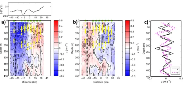
The ADCP zonal (Fig. 4a) and meridional (Fig. 4b) currents show a baroclinic, anticyclonic rotating 30

flow, with a maximum swirl velocity of about 0.45 m s^-1 at about 100 m depth. The maximum rotation speed (approximately represented by the zonal section) decreases nearly linear to about 380 m depth where 0.1 m s^-1 is reached. Alternating currents with about 80 to 100 m wavelength can be seen close to the eddy edges and more clearly seen after subtracting 120 m boxcar filtered profiles (Fig. 4 c). The

9

local (at 19°N) inertial period is 36.7 h while the ADCP section was surveyed in 14 h (including station time) and only a moderate aliasing effects is expected in the sections. In contrast, the glider took more than 5 days (4 inertial periods) to complete the section (Fig. 3) and a mixture of time/space variability is mapped.

Considering the translation speed of the eddy of 3 to 5 km day^-1 (see Fiedler et al. 2016) the nonlinearity 5

parameter 𝛼, relating maximum swirl velocity to the translation speed, is much larger than 1 (about 6.5 to 11 in the depth level of the low oxygen core) and indicates a high coherence of the eddy. At the depth of the maximum swirl velocity, and considering the eddy radius of 30 km, a full rotation would take about 5 days but for the deeper levels more.

3.2 Eddy core isolation and vertical fluxes 10

The concept proposed for the formation of the low oxygen zone is based on an isolation of the eddy core, in combination with high productivity and subsequent respiration of sinking organic material – in analogy to the formation of dead-zones in coastal and limnic systems (Karstensen et al. 2015). The water mass observed in the ACME defines a strong anomaly against the surrounding waters and is very similar to water masses at the eastern boundary, where the ACME was formed (Fiedler et al. 2016). The 15

constancy of hydrographic properties over a period of about 7 month have been shown for this ACME (Fiedler et al. 2016) and suggests that no significant exchange between eddy core and surrounding water through either lateral or diapycnal processes occurred.

The high nonlinearity parameter for the eddy (𝛼≫1) indicates its coherence and explains why the eddy was so remarkably stable when comparing observations of the eddy 2 month apart (Fig. 2).

20

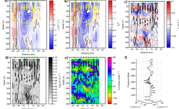
However, the high 𝛼 does not explain the isolation of the core against mixing. Mixing in the thermocline is closely related to breaking of internal waves (Gregg et al. 1986, Gregg 1989), maybe with local enhancement by double diffusive mixing in cases where vertical gradients are intense (St Laurent and Schmitt 1999). To determine the possible interaction of the low oxygen eddy with the internal wave field we first calculate the relative vorticity 𝜁 of the eddy (Fig. 5a) and then investigated 25

the impact on the local 𝑓. The anticyclonic (negative) 𝜁 in the core of the low oxygen eddy is about

−0.8∙𝑓 (Ro = –0.8) and changes sign at the boundary of the core, where large Ro remain (Ro ~0.4) suggesting that eddy rotational effect are important. The 𝑓!"" in the ACME (Fig. 5b) is lowered to values of 0.6 in the core (Kunze et al 1995), while underneath the core, and below the lower N² maximum, still values of 0.8 are found. Such low 𝑓!"" force NIW to propagate downward also called 30

“inertial chimney” (Lee and Niller 1998). In contrast to a typical AE stratification (Kunze 1985, Kunze et al. 1995, Joyce et al. 2013) the low oxygen ACME has an intense N² maximum (10^-4 s^-2) defining its upper boundary and that also aligns with the mixed layer base (Fig. 3c). Model studies (Lee and Niiler 1998) and ray tracing analysis (Sheen et al. 2015) show for ACME that most of the NIW energy

10

accumulates below the eddy. As a consequence, mixing inside the core is low and is well separated from mixing outside the core. This separation of mixing regimes we interpret as why the low oxygen eddy core has been so constant in its water mass properties.

Having now the isolation explained as a consequence of eddy rotation and stratification and their joint impact on the propagation of internal waves, it is tempting to investigate whether the vertical flux of 5

nutrients into the euphotic layer of the eddy may also fit to this concept. The productivity associated with the ACME requires intense episodic or prolonged moderate upward fluxes of nutrients into the euphotic zone. From global assessments of productivity in mesoscale eddies based on satellite data (Chelton et al. 2011b; Gaube et al. 2015) the upwelling is identified in the centre of the eddies. Note, that these studies do not explicitly consider ACME. Schütte et al. (2016) showed that low oxygen 10

ACME do have productivity maxima (indicated by enhanced ocean color based Chlorophyll-a estimated) at the rim of the eddies, not at the centre. This may suggest that the vertical flux is also concentrated to the rim. Inspecting the glider section data (Fig. 3) does not show indications for upwelling in the centre, isopycnals in the core are flat and the core has only a weak (and vertical) stratification. The mixed layer base is characterized by the very stable stratification and large gradients 15

(e.g. 0.3 K m^-1 in temperature). The ship’s thermosalinograph temperature data (Fig. 3a upper) show the eddy to be colder than the surroundings but also indicate that a local maximum in temperature is observed in the centre of the eddy, while local minima (0.2 K difference) at ±15 km distance from the centre. Considering the first glider oxygen section (IFM12, Fig. 2a), the upper of the two separate minima is found very close to the depth of the mixed layer base and indicate that any exchange across 20

the mixed layer by mixing processes must be very small.

Following up on the NIW discussion, we now consider the region outside the core and in the vicinity of the eddy. It is a reasonable assumption that a large fraction of the NIW energy originates from wind stress fluctuations (D’Asaro 1985). The NIW propagation in the upper layer of the eddy (above the core) is primarily along the intense N contours/mixed layer base (Fig. 3c) and towards the eddy rim 25

(shown in Sheen et al. 2015). At the eddy rim, but outside of the maximum N contour, the NIW can propagate downward (see Fig. 4 b,d) because 𝑓!""<1 (Fig. 5b). In this zone we observed the impact of the vertical propagation in the vertical shear profile directly via the modulation of the maximum swirl velocity (approximately Fig. 3a, at ~ –32 km distance).

In order to extract the velocity signal related to the NIW (𝑈^!), we subtracted the filtered (120 m boxcar 30

filter) velocity profile data (𝑈_!) from the observed profiles (𝑈; Fig. 5c):

𝑈=𝑈_!+𝑈^!

Magnitude and angle between the zonal and meridional NIW components of 𝑈^! show a vertically stacked pattern within the 𝑓!"" region, suggesting the trapping of the NIW underneath the eddy (Lee

11

and Niiler 1998). The phase angle and its cyclonic rotation with depth indicate a downward propagation of the waves (Joyce et al. 2013). Another region where rotation and a maximum in amplitude is seen is the outer rim of the eddy in the region where 𝑓!"" approaches 1, in the depth range between 50 and 120 m (~ –30 km). The NIWs have an amplitude of more than 0.1 m s^-1 and a vertical scale of about 70 to 90 m (Fig. 4d), similar to observations at mid latitude fronts (Kunze and Sanford 1984). The 5

inertial radius for a wave with amplitude of 0. 1 m s^-1 is about 2 km. The NIW wave pattern underneath the eddy core aligns well with the pattern observed in the glider sections (Fig 2 and 3).

A Richardson gradient number 𝑅𝑖_!=𝑁^!/( ^!"_!" ^!+ ^!"_!" ^!) cannot directly be estimated along the sections because no concurrent velocity and stratification section data exists. Considering single profile data the shear in velocity is about 0.1 m s^-1 over 50 to 70 m depth (Fig. 3d) equals a variance of 10

0.2−0.4∙10^!! s^-2 that is implied along the wave propagation path. Outside of the mixed layer base N² maximum, a corresponding 𝑅𝑖_!<10 can be expected to occur (see Fig. 2c), a value that may indicate generation of instabilities (Joyce et al. 2013).

Only vertical propagation of internal waves does not generate mixing, but the waves have to either break (Kelvin-Helmholtz instabilities) or produce enough shear to generate critical layer absorption.

15

When considering the maximum velocities (0.1m s^-1) associated with the NIW they account for about 25% of maximum swirl velocity. However, a region close to, but outside of, the maximum swirl velocity (about ~ –32 km, 50 to 120m depth) is identified where 𝑓_!"!<1 and the NIW velocity (𝑈^!) is of similar magnitude as the flow (𝑈) and thus susceptible for critical layer formation. Here the mean flow could gain energy from the NIW but also vertical mixing. It has been shown that trapping of NIW 20

inside an AE (Gulf Stream warm core ring, Joyce et al. 2013) generated most instabilities and mixing close to surface and where most horizontal shear in the baroclinic current is found. In case of the ACME discussed here, this is close to the mixed layer base and at 90 m depth (Fig. 4a) and potentially opening a pathway for properties from below into the mixed layer (and vice versa). Some evidence for such a flux can be seen in the nitrate section (Fig. 6 b) that show a local maximum maybe associated 25

with an upward filament at about 100 m depth/distance of about –32 km.

An asymmetry in the dynamical structure is seen for example in the 𝑓!"" section (Fig. 5b). All sections run from south (most negative distance) to north and it is the southern part that is more coherent and energetic and this is also the flank were the NIW signal is strongest. It is possible that the interaction of the eddy with the north-easterly trade winds play a role here because the eddy frontal flow is in the 30

direction of the wind. Thomas (2005) showed the generation of a vertical flux at the mixed layer base that entrains water from underneath.

Below the eddy the SA gradients (Fig. 3a) do align well with the wave crests and that may indicate the impact of intense strain, and an thus a periodic intensification of SA gradients which in turn could

12

enhance the susceptibility to double diffusive mixing in regions where susceptibility of double diffusion is already indicated by the Tu distribution (Fig. 3d).

3.3 A nutrient budget for the eddy

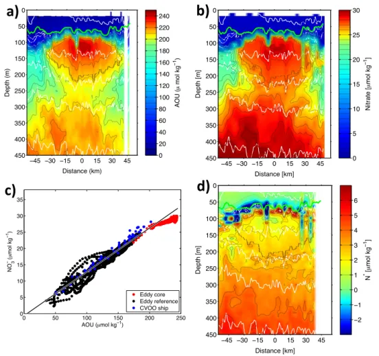
In order to interpret the low oxygen concentrations in terms of biogeochemical processes, we calculated the apparent oxygen utilization (AOU, Fig. 6a), which is defined as the difference between measured 5

oxygen concentration and the oxygen concentration of a water parcel of the given θ and SA that is in equilibrium with air (Garcia and Gordon, 1992; 1993). AOU is an approximation for the total oxygen removal since a water parcel left the surface ocean. The low oxygen concentrations in the core of the eddy are equivalent to an AOU of about 240 µmol kg^-1 (Fig 6a). Along with high AOU we also find very high NO₃^- concentrations with a maximum of about 30 µmol kg^-1 (Fig 6b). The corresponding 10

AOU:NO₃^- ratio outside the core is 8.1 and thus close to the classical 8.625 Redfield ratio (138/16;

Redfield et al. 1938). However, in the core an AOU: NO3- ratio of >16 is found. This high ratio indicates that less NO3- is released during respiration (AOU increase) than expected for a process following a Refieldian stoichiometry. By considering a linear fit to outside the core (Fig. 6c) the respective NO3- deficit can be estimated to up to 4-6 µmol kg^-1 for the highest AOU (NO3-) 15

observations. By integrating NO3- and NO3--deficit over the core of the low oxygen eddy (defined here as the volume occupied by water with oxygen concentrations < 40 µmol kg^-1) we obtain a average AOU: NO3- ratio of about 20:1.

One way to interpret this deficit is by NO₃^- loss through denitrification processes. Loescher et al. (2015) and Grundle et al. (in revision) both found evidence for the onset of denitrification in the core of the 20

ACME discussed here. Oxygen concentrations in the core are very low (about 3 µmol kg^-1) and denitrification is possible. Evidence for denitrification in the core of the ACME was, however, demonstrated as being important for N2O cycling at the nanomolar range (Grundle et al. in revision), and not necessarily for overall NO3- losses which are measured in the micromolar range. Estimates of N* from the ACME show that even in the core of the ACME NO3-- losses were not detectable at the 25

micromolar range (Fig. 6d). Thus, while denitrification may have played a minor role in causing the higher than expected AOU:NO3- ratio which we have calculated, it is unlikely that it contributed largely to the loss of 5% of all NO3- from the eddy as estimated based on the observed AOU:NO3- ratios.

Alternatively, but perhaps not exclusively, the NO3- recycling within the ACME could be the reason for the NO3- deficit. A high AOU: NO3- ratio could be explained through a decoupling of NO3- and oxygen 30

recycling pathways in the eddy. In this scenario NO3- molecules are used more than one time for the remineralization/respiration process and therefore the AOU increase without a balanced NO3-

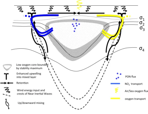
remineralization. Such a decoupling can be conceptualized as follows (Fig. 7): consider an upward flux of dissolved NO3- and oxygen in a given ratio with an amount of water that originates from the low

13

oxygen core. The upward flux partitions when reaching the mixed layer, one part disperses in the open waters outside of the eddy, the other part is keep in the eddy by retention (D'Ovidio et al. 2013). The upwelled NO3- is utilized by autotrophs for primary production and thereby incorporated into particles (PON) while the corresponding oxygen production is ventilated to the atmosphere. The PON sinks out of the mixed layer/euphotic zone and into the core of the eddy were remineralization of organic matter 5

releases quickly some of the same NO3- back into the core. In contrast, the upwelling of oxygen- deficient waters will drive an oxygen flux from the atmosphere into the ocean in order to reach chemical equilibrium. But because the stoichiometric equivalent of oxygen is lost to the atmosphere and therefore not transported back into the core by gravitational settling of particles, as is the case for nitrate (via PON), the respiration associated with the remineralization of the recycled nitrate will results in a 10

net increase in AOU. A potential problem with this concept is that the NO3-/oxygen from the eddy core is primarily outward, so it must be more an erosion rather then a flux, because a flux would also transport from outside into the core and thus slowly altering the core properties (which is not observed).

It could be an erosion process that maintains an stability maximum along with the exchange and maybe related to interleaving (Beal 2007). Further work is needed to understand this process in full.

15

4 Summary and Conclusion

Here we present a first analysis of high-resolution multidisciplinary glider and ship survey data of a low oxygen anticyclonic mode-water eddy (ACME) in the eastern tropical North Atlantic. The eddy has a diameter of about 70 to 80 km and maximum swirl velocity of 0.4 m s^-1 (at about 90 m depth) and can be considered typical for the region (Schütte et al. 2015, 2015; Karstensen et al. 2015). The eddy 20

originated from the Mauritanian upwelling region (Schütte et al. 2016; Fiedler et al. 2016) and had a distinct, anomalously fresh (and cold), water mass in its core that was located immediately below the mixed layer base (about 70 to 80 m) and a depth of 200 to 250 m. The core showed minimum oxygen concentrations of 8 µmol kg^-1 during the first glider survey (February 2014) and 3 µmol kg^-1 during the second glider survey, 9 weeks later. Enhanced productivity was estimated for the eddy (Fiedler et al.

25

2016), implying a vertical flux of nutrient rich waters to the euphotic zone/mixed layer. A concept for the isolation of the core but enhanced vertical flux of nutrients in parallel was derived (Fig. 7). The velocity observations indicate that the eddy had a very distinct impact on the propagation of near inertial internal waves as expected (Kunze 1985, Kunze et al. 1995, Sheen et al. 2015). The combination of a negative vorticity anomaly of an anticyclonic rotating eddy and a maximum in 30

stratification that encloses the ACME’s low oxygen core on the one side traps the NIW to the eddy vicinity but also prevent NIW to enter the core. A velocity shear variance maximum is found below the eddy that is interpreted as an NIW energy maximum, as seen from model simulations of NIW propagation around ACME (Lee and Niiler 1998). Outside the low oxygen core, at the upper bound of the stability maximum, we expect enhanced mixing to occur, as shown for ACME in the deep ocean 35

14

(Sheen et al. 2015). Moreover, for AE it has been reported that in the depth range were the NIW interact with the maximum baroclinic flow (in our case at about 90 m) enhanced mixing can occur (Joyce et al.

2013) possibly by critical layer formation. Our analysis suffers from not having concurrent hydrography and currents data, and limited options for estimating balances (e.g. Richardson numbers) exists.

However, if we transfer the findings by Joyce et al. (2013) to our eddy the enhanced mixing would be at 5

the mixed layer base, but outside the eddy. An asymmetry in the dynamical structure of the eddy is observed (not so much in hydrography though) with a more intense front in the southern part of the section and which is directly under the impact of the Ekman flow generated by the Norteast Trade winds. A NIW induced mixing would create an upward flux of nutrients, also supported by the NO₃^- distribution. Once NO3-is in the mixed layer the eddy retention (D’Ovidio et al. 2013) will trap a 10

fraction of the upwelling waters. The AOU:NO3- ratio of the eddy core is altered high (16) when compared with the classical Redfield ratio (8.625) or the background ratio (8.1). We estimated the NO3-

deficit for the eddy which is about 1:20 when referenced to the total NO3- content. Denitrification is one possible process but the significant nitrate loss of the core seems unrealistic. What is more likely is a local recycling of N but not oxygen and connected to the transfer of upwelled NO3- from the core via 15

sinking of PON. The isolation of the eddy core in combination with high productivity is a prerequisite for the formation of the low oxygen core and as such analogue to the formation of a “dead-zones”, known to occur in coastal and limnic systems (Karstensen et al. 2015). The isolated core is the rare case of an isolated volume of water in the open ocean and which allow to study fundamental biogeochemical cycling processes in the absence of significant physical transport processes. A number of surprising 20

biogeochemical cycling processes and ecosystem responses have been reported from the studies on eastern tropical North Atlantic low-oxygen eddies (Löscher et al. 2015, Hauss et al. 2016, Fiedler et al.

2016; Fischer et al. 2016, Grundle et al. in revision, Schütte et al. 2016). The NIW concept for the vertical flux outside the core but likewise the isolation of the ACME core that we presented here is based on internal wave processes that are not routinely resolved by numerical models. A strategy for 25

parameterizing of these processes is however required considering the estimate by Schütte et al. (2016) who showed that the enhanced respiration in low oxygen eddies contribute about 20% to net respiration that creates the shallow oxygen minimum of the eastern tropical Atlantic.

Acknowledgment

We thank the authorities of Cape Verde for the permission to work in their territorial waters. We 30

acknowledge the support of the captains and crews of R/V Islandia (glider survey support) and R/V Meteor. We thank Tim Fischer (GEOMAR) for processing the ADCP data and Marcus Dengler for fruitful discussions. Financial support for this study was provided by a grant from the Cluster of Excellence “The Future Ocean” to J. Karstensen, A. Körtzinger, C.R. Löscher, and H. Hauss. Glider data analysis where supported by the DFG Collaborative Research Centre754 (www.sfb754.de). B.

35

15

Fiedler was funded by the Germany Ministry for Education and Research (BMBF) project SOPRAN (grant no. 03F0662A). F. Schütte and P. Testor were supported by the trilateral project AWA supported by BMBF (grant no. 01DG12073E). Analysis was supported by European Union's Horizon 2020 research and innovation programme under grant agreement No 633211 (AtlantOS).

5

References

Alford, M.H., J.A. MacKinnon, H.L. Simmons, J.D. Nash, Near-Inertial Internal Gravity Waves in the Ocean, Annual Review of Marine Science 8, 95-123, 2016

Armi, L., and W. Zenk, Large lenses of highly saline Mediterranean water. J. Phys. Oceanogr., 14, 1560–1576, doi:10.1175/1520-0485(1984)014,1560:LLOHSM.2.0.CO;2., 1984

10

Beal, L.M., Is Interleaving in the Agulhas Current Driven by Near-Inertial Velocity Perturbations?. J.

Phys. Oceanogr., 37, 932–945. doi: http://dx.doi.org/10.1175/JPO3040.1, 2007.

Booker, J.R. and Francis P. Bretherton, The critical layer for internal gravity waves in a shear flow.

Journal of Fluid Mechanics, 27, pp 513-539 doi:10.1017/S0022112067000515, 1967.

Chaigneau, A., Eldin, G. and Dewitte, B.: Eddy activity in the four major upwelling systems from 15

satellite altimetry (1992–2007), Prog. Oceanogr., 83(1-4), 117–123, doi:10.1016/j.pocean.2009.07.012, 2009

Chaigneau, A., Le Texier, M., Eldin, G., Grados, C., and Pizarro, O.: Vertical structure of mesoscale eddies in the eastern South Pacific Ocean: A composite analysis from altimetry and Argo profiling floats, Journal of Geophysical Research: Oceans, 116, C11025, 2011.

20

Chelton, D. B., Schlax, M. G. and Samelson, R. M.: Global observations of nonlinear mesoscale eddies, Prog. Oceanogr., 91(2), 167–216, doi:10.1016/j.pocean.2011.01.002, 2011a

Chelton, D., P. Gaube, M. Schlax, J. Early, and R. Samelson, The influence of nonlinear mesoscale eddies on near-surface oceanic chlorophyll. Science, 334, 328–332, doi:10.1126/ science.1208897, 2011b

25

Dewar, W.K. and G. R. Flierl, Some Effects of the Wind on Rings. J. Phys. Oceanogr., 17, 1653–1667.

doi: http://dx.doi.org/10.1175/1520-0485, 1987.

D’Asaro, E., The energy flux from the wind to near-inertial motions in the mixed layer, J. Phys.

Oceanogr., 15, 943–959, 1985.

D’Asaro, E.A., Generation of submesoscale vorticies: a new mechanism. J. Geophys. Res. 93, 6685–

30

6693, 1988.

D'Ovidio F., De Monte S., Della Penna A., Cotté C. and Guinet C., Ecological implications of oceanic eddy retention in the open ocean: a Lagrangian approach. J. Phys. A: Math. Theor. 46: 254023 (doi:10.1088/1751-8113/46/25/254023), 2013.

16

Eden, C., and H. Dietze, Effects of mesoscale eddy/wind interactions on biological new production and eddy kinetic energy, J. Geophys. Res., 114, C05023, doi:10.1029/2008JC005129., 2009.

Fiedler, B., Grundle, D., Schütte, F., Karstensen, J., Löscher, C. R., Hauss, H., Wagner, H., Loginova, A., Kiko, R., Silva, P., and Körtzinger, A.: Oxygen Utilization and Downward Carbon Flux in an Oxygen-Depleted Eddy in the Eastern Tropical North Atlantic, Biogeosciences Discuss., 5

doi:10.5194/bg-2016-23, in review, 2016.

Fischer, G., Karstensen, J., Romero, O., Baumann, K.-H., Donner, B., Hefter, J., Mollenhauer, G., Iversen, M., Fiedler, B., Monteiro, I. and Körtzinger, A.: Bathypelagic particle flux signatures from a suboxic eddy in the oligotrophic tropical North Atlantic: production, sedimentation and preservation, Biogeosciences Discuss., 12(21), 18253–18313, doi:10.5194/bgd-12-18253-2015, 10

2015.

Garcia, H.E., and L.I. Gordon, Oxygen solubility in seawater: Better fitting equations. Limnology and Oceanography, 37, 1307-1312, 1992.

Garcia, H.E., and L.I. Gordon, Erratum: Oxygen solubility in seawater: better fitting equations.

Limnology and Oceanography, 38, 656, 1993.

15

Gaube, P., D.B. Chelton, R. M. Samelson, M.G. Schlax, and L.W. O’Neill, Satellite Observations of Mesoscale Eddy-Induced Ekman Pumping. J. Phys. Oceanogr., 45, 104–132. doi:

http://dx.doi.org/10.1175/JPO-D-14-0032.1, 2015.

Gregg, M.C., E.A. D'Asaro, T.J. Shay, and N. Larson, Observations of Persistent Mixing and Near- Inertial Internal Waves. J. Phys. Oceanogr., 16, 856–885. doi: http://dx.doi.org/10.1175/1520- 20

0485(1986)016<0856:OOPMAN>2.0.CO;2, 1986.

Gregg, M. C., Scaling turbulent dissipation in the thermocline, J. Geophys. Res., 94(C7), 9686–9698, doi:10.1029/JC094iC07p09686, 1989.

Hahn, J., Brandt, P., Greatbatch, R., Krahmann, G., and Körtzinger, A., Oxygen variance and meridional oxygen supply in the Tropical North East Atlantic oxygen minimum zone, Climate 25

Dynamics, 43, 2999–3024, 2014.

Hauss, H., Christiansen, S., Schütte, F., Kiko, R., Edvam Lima, M., Rodrigues, E., Karstensen, J., Löscher, C. R., Körtzinger, A. and Fiedler, B.: Dead zone or oasis in the open ocean? Zooplankton distribution and migration in low-oxygen modewater eddies, Biogeosciences Discuss., 12(21), 18315–18344, doi:10.5194/bgd-12-18315-2015, 2016.

30

Hua, B. L., C. Menesguen, S. L. Gentil, R. Schopp, B. Marsset, and H. Aiki, Layering and turbulence surrounding an anticyclonic oceanic vortex: in situ observations and quasi-geostrophic numerical simulations, J. Fluid Mech., 731, 418-442, 2013.

IOC, SCOR and IAPSO, The international thermodynamic equation of seawater – 2010: Calculation and use of thermodynamic properties. Intergovernmental Oceanographic Commission, Manuals 35

and Guides No. 56, UNESCO (English), 196 pp., 2010.

17

Johnson, K. S., L. J. Coletti, H, W. Jannasch, C.M. Sakamoto, D. Swift, S. C. Riser, Long-term nitrate measurements in the ocean using the In Situ Ultraviolet Spectrophotometer: sensor integration into the Apex profiling float. Journal of Atmospheric and Oceanic Technology, 30, 1854-1866, 2013.

Joyce, T. M., J. M. Toole, P. Klein, and L. N. Thomas, A near-inertial mode observed within a Gulf Stream warm-core ring, J. Geophys. Res. Oceans, 118, 1797–1806, doi:10.1002/jgrc.20141, 2013.

5

Karstensen, J., Fiedler, B., Schütte, F., Brandt, P., Körtzinger, A., Fischer, G., Zantopp, R., Hahn, J., Visbeck, M., and Wallace, D.: Open ocean dead zones in the tropical North Atlantic Ocean, Biogeosciences, 12, 2597-2605, 2015.

Kostianoy, A., Belkin, I., A survey of observations on intrathermocline eddies in the world ocean. In Mesoscale/Synoptic Coherent Structures in Geophysical Turbulence, Nihoul, J., Jamart, B. (eds.) 10

Vol. 50, 821–841 (Elsevier, New York). 1989.

Koszalka, I. M., Ceballos, L. and Bracco, A., Vertical mixing and coherent anticyclones in the ocean:

the role of stratification Nonlinear Processes in Geophysics, 17 (1). pp. 37-47. DOI 10.5194/npg- 17-37-2010, 2010.

Krahmann, G., P. Brandt, D. Klaeschen, and T. Reston, Mid-depth internal wave energy off the Iberian 15

Peninsula estimated from seismic reflection data, J. Geophys. Res., 113, C12016, doi:10.1029/2007JC004678, 2008.

Kunze, E., Near-inertial wave propagation in geostrophic shear, J. Phys. Oceanogr., 15, 544–565, 1985.

Kunze, E., R. W. Schmidt, and J. M. Toole, The energy balance in a warm core ring’s near-inertial critical layer. J. Phys. Ocean- ogr., 25, 942–957, 1995.

20

Ledwell J.R., D.J. McGillicuddy Jr., L.A. Anderson, Nutrient flux into an intense deep chlorophyll layer in a mode-water eddy, Deep-Sea Research, 55, 1139–1160, 2008.

Lee, D., and P. Niiler, The inertial chimney: The near-inertial energy drainage from the ocean surface to the deep layer. J. Geophys. Res., 103 (C4), 7579–7591, 1998.

Lévy, M., Ferrari, R., Franks, P. J. S., Martin, A. P., and Rivière, P.: Bringing physics to life at the 25

submesoscale, Geophys. Res. Lett., 39, L14602, doi:10.1029/2012GL052756, 2012.

Löscher, C. R., Fischer, M. A., Neulinger, S. C., Fiedler, B., Philippi, M., Schütte, F., Singh, A., Hauss, H., Karstensen, J., Körtzinger, A., Künzel, S. and Schmitz, R. A.: Hidden biosphere in an oxygen- deficient Atlantic open ocean eddy: future implications of ocean deoxygenation on primary production in the eastern tropical North Atlantic, Biogeosciences, 12, 7467-7482, doi:10.5194/bg- 30

12-7467-2015, 2015.

Mahadevan, A., Thomas, L. N., Tandon, A., Comment on Eddy/Wind Interactions Stimulate Extraordinary Mid-Ocean Plankton Blooms. Science 320, 448, 2008.

McDougall, T.J. and P.M. Barker, Getting started with TEOS-10 and the Gibbs Seawater (GSW) Oceanographic Toolbox, 28 pp., SCOR/IAPSO WG127, ISBN 978-0-646-55621-5, 2011.

35

McDougall, T.J., and O.A. Krzysik, Spiciness. Journal of Marine Research, 73, 141-152, 2015.

18

McDougall, T. J., Jackett, D. R., Millero, F. J., Pawlowicz, R., and Barker, P. M.: A global algorithm for estimating Absolute Salinity, Ocean Sci., 8, 1123-1134, doi:10.5194/os-8-1123-2012, 2012.

McGillicuddy, D. J., Anderson, L. A., Bates, N. R., Bibby, T., Buesseler, K. O., Carlson, C. A., Davis, C. S., Ewart, C., Falkowski, P. G., Goldthwait, S. A., Hansell, D. A., Jenkins, W. J., Johnson, R., Kosnyrev, V. K., Ledwell, J. R., Li, Q. P., Siegel, D. A. and Steinberg, D. K.: Eddy/Wind 5

Interactions Stimulate Extraordinary Mid-Ocean Plankton Blooms, Science, 316 (5827), 1021–

1026, doi:10.1126/science.1136256, 2007.

McWilliams, J.C., Submesoscale, coherent vortices in the ocean, Rev. Geophys., 23(2), 165–182, doi:10.1029/RG023i002p00165. 1985.

Redfield, A. C., Ketchum, B. H. and Richards, F. A.: The influence of organisms on the composition of 10

seawater, in The Sea. Interscience, edited by M. N. Hill, pp. 26–77, 1963.

Sakamoto, C.M., Johnson, K.S. and Coletti, L.J., An improved algorithm for the computation of nitrate concentrations in seawater using an in situ ultraviolet spectrophotometer. Limnol. Oceanogr.

Methods 7, 132-143, 2009.

Schütte, F., Karstensen, J., Krahmann, G., Hauss, H., Fiedler, B., Brandt, P., Visbeck, M., and 15

Körtzinger, A.: Characterization of “dead-zone” eddies in the tropical Northeast Atlantic Ocean, Biogeosciences Discuss. , doi:10.5194/bg-2016-33, in review , 2016.

Schütte, F., Brandt, P. and Karstensen, J.: Occurrence and characteristics of mesoscale eddies in the tropical northeast Atlantic Ocean, Ocean Sci. Discuss., 12(6), 3043–3097, doi:10.5194/osd-12- 3043-2015, 2015.

20

Sheen, K. L., J. A. Brearley, A. C. Naveira Garabato, D. A. Smeed, L. St Laurent, M. P. Meredith, A.

M. Thurnherr, and S. N. Waterman, Modification of turbulent dissipation rates by a deep Southern Ocean eddy, Geophys. Res. Lett., 42, 3450–3457, doi:10.1002/2015GL063216, 2015.

St. Laurent, L., and R.W. Schmitt, 1999: The Contribution of Salt Fingers to Vertical Mixing in the North Atlantic Tracer Release Experiment. J. Phys. Oceanogr., 29, 1404–1424. doi:

25

http://dx.doi.org/10.1175/1520-0485(1999)029<1404:TCOSFT>2.0.CO;2, 1999

Thomas, L. N., 2005: Destruction of potential vorticity by winds. J. Phys. Oceanogr., 35, 2457– 2466.

Thomas, L. N., Formation of intrathermocline eddies at ocean fronts by wind-driven destruction of potential vorticity, Dynam. Atmos. Oceans, 45, 252-273, 2008.

Whitt, D. B., and L. N. Thomas, Near-inertial waves in strongly baroclinic currents, Journal Physical 30

Oceanography, doi:10.1175/JPO-D-12-0132.1, 2013

Zhang, Z., Zhang, Y., Wang, W., and Huang, R. X.: Universal structure of mesoscale eddies in the ocean, Geophysical Research Letters, 40, 3677-3681, 2013.

19 Figures

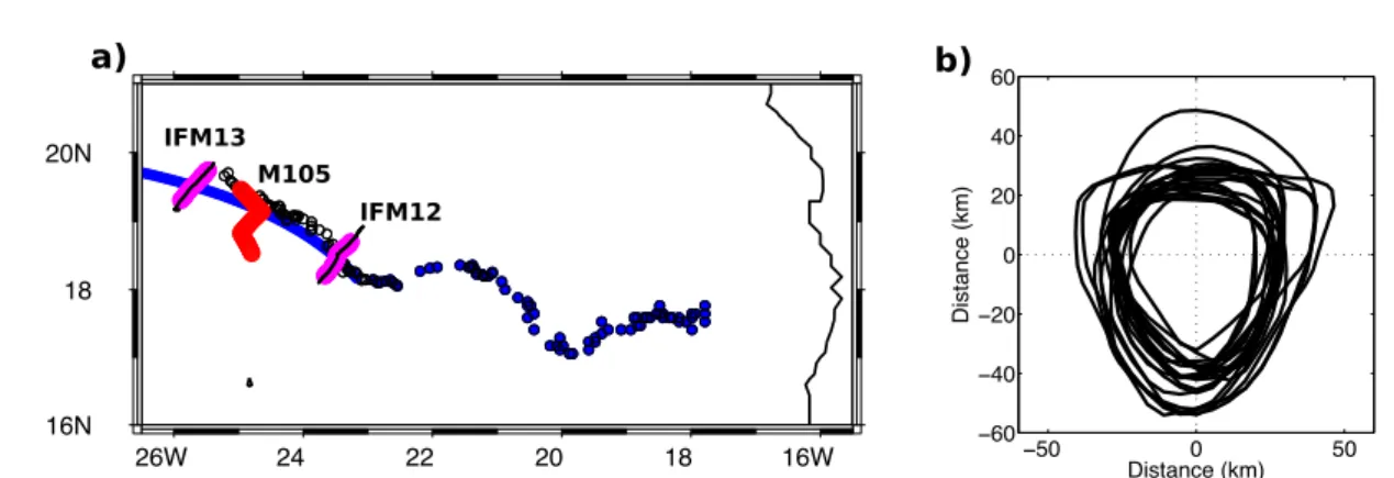
Figure 1 (a) Location of the two glider surveys (black dots and magenta dots; IFM12, IFM13) and the ship survey (red dots;

5

M105) in geographical context with our best estimate of the eddy centre trajectory from sea level anomaly data (see e.g. Fiedler et al. 2016). The smoothed trajectory west of about 23°W is derived from visible inspection, elsewhere it is based on an automatic tracking algorithms (see Schütte et al. 2015, 2016). (b) The eddy diameter from sea level anomaly data during the IMF12 survey projected on the eddy centre.

10

−50 0 50

−60

−40

−20 0 20 40 60

Distance (km)

Distance (km)

26W 24 22 20 18 16W

16N 18 20 N

a) b)

IFM13

IFM12 M105

20

5 Figure 2: Oxygen distribution from the three surveys (locations of the surveys see Fig. 1) over a similar distance (-55 to 55 km relative to a subjectively selected eddy centre) a) IFM12, b) M105, and c) IFM13. The 15 µmol kg^-1 (40 µmol kg^-1) oxygen contour is indicated as bold (stippled) line, selected density anomaly contours are shown as white lines (∆σ = 0.2 kg m^-3). The green line indicates the mixed layer depth. The oxygen contour in b) was gridded based on the 8 stations (locations indicated by green stars) and mapped to a linear section in latitude, longitude. The yellow dots indicate positions of local stability maxima.

10

Distance (km)

Depth (m)

−45 −30 −15 0 15 30 45 0

50 100 150 200 250 300 350 400 450

Oxygen (µmol kg−1)

0 25 50 100 150 200

Distance (km)

Depth (m)

−40 −20 0 20 40

0 50 100 150 200 250 300 350 400 450

Oxygen (µmol kg−1)

0 25 50 100 150 200

Distance (km)

Depth (m)

−45 −30 −15 0 15 30 45 0

50 100 150 200 250 300 350 400 450

Oxygen (µmol kg−1)

0 25 50 100 150

a) b)

c)

21

Figure 3: a) SA, b) spiciness, c) buoyancy frequency/stability (N²), d) Turner angle (only segment |45| to |90| is shown). All section are from IFM12. The thick black broken line indicates the 40 µmol kg^-1 oxygen concentration (see Fig. 2). Colour coding and selected contours see individual colour bar. Selected density anomaly contours are shown as white lines (∆σ = 0.2 kg m^-3). The green line indicates the mixed layer depth.

5

Distance (km)

Depth (m)

−45 −30 −15 0 15 30 45 0

50 100 150 200 250 300 350 400 450

N2 (10−5 s−1)

0 1 2 3 4 5 6 7 8 9 10 11 12

Distance (km)

Depth (m)

−45 −30 −15 0 15 30 45 0

50 100 150 200 250 300 350 400 450

Spiciness (kg m−3)

1 1.5 2 2.5 3 3.5 4 4.5 5

Distance (km)

Depth (m)

−45 −30 −15 0 15 30 45 0

50 100 150 200 250 300 350 400 450

Absolute Salinity (gr kg−1)

35.2 35.4 35.6 35.8 36 36.2 36.4 36.6

a)

b)

c) d)

Distance [km]

Depth [m]

−45 −30 −15 0 15 30 45 0

50 100 150 200 250 300 350 400 450

Turner angle

−90

−45 0 45 90