Nitrogen cycling in shallow low-oxygen coastal waters off Peru from nitrite and nitrate nitrogen and oxygen isotopes

(1)

www.biogeosciences.net/13/1453/2016/

doi:10.5194/bg-13-1453-2016

Nitrogen cycling in shallow low-oxygen coastal waters off Peru from nitrite and nitrate nitrogen and oxygen isotopes

Happy Hu^1,*, Annie Bourbonnais^1,*, Jennifer Larkum¹, Hermann W. Bange², and Mark A. Altabet¹

1School for Marine Science and Technology, University of Massachusetts Dartmouth, 706 South Rodney French Blvd, New Bedford, MA 02744-1221, USA

2GEOMAR Helmholtz Centre for Ocean Research Kiel, Düsternbrooker Weg 20, 24105 Kiel, Germany

*These authors contributed equally to this work.

Correspondence to: Annie Bourbonnais (abourbonnais@umassd.edu)

Received: 17 April 2015 – Published in Biogeosciences Discuss.: 18 May 2015 Revised: 14 January 2016 – Accepted: 7 February 2016 – Published: 9 March 2016

Abstract. O₂deficient zones (ODZs) of the world’s oceans are important locations for microbial dissimilatory nitrate (NO⁻₃)reduction and subsequent loss of combined nitrogen (N) to biogenic N₂ gas. ODZs are generally coupled to regions of high productivity leading to high rates of N-loss as found in the coastal upwelling region off Peru. Stable N and O isotope ratios can be used as natural tracers of ODZ N- cycling because of distinct kinetic isotope effects associated with microbially mediated N-cycle transformations. Here we present NO⁻₃ and nitrite (NO⁻₂)stable isotope data from the nearshore upwelling region off Callao, Peru. Subsurface oxygen was generally depleted below about 30 m depth with concentrations less than 10 µM, while NO⁻₂ concentrations were high, ranging from 6 to 10 µM, and NO⁻₃ was in places strongly depleted to near 0 µM. We observed for the first time a positive linear relationship between NO⁻₂δ¹⁵N andδ¹⁸O at our coastal stations, analogous to that of NO⁻₃ N and O isotopes during NO⁻₃ uptake and dissimilatory reduction. This relationship is likely the result of rapid NO⁻₂ turnover due to higher organic matter flux in these coastal upwelling waters. No such relationship was observed at offshore stations where slower turnover of NO⁻₂ facilitates dominance of isotope exchange with water. We also evaluate the overall isotope fractionation effect for N-loss in this system using several approaches that vary in their underlying assumptions.

While there are differences in apparent fractionation factor (ε) for N-loss as calculated from theδ¹⁵N of NO⁻₃, dissolved inorganic N, or biogenic N2, values forεare generally much lower than previously reported, reaching as low as 6.5 ‰. A possible explanation is the influence of sedimentary N-loss at

our inshore stations which incurs highly suppressed isotope fractionation.

1 Introduction

Chemically combined nitrogen (N), e.g., nitrate (NO⁻₃), is an important phytoplankton nutrient limiting primary productivity and carbon export throughout much of the ocean (e.g.

Gruber, 2008). The marine nitrogen cycle involves a series of microbial processes, which transfer N between a num- ber of chemical forms. These include N₂fixation, nitrifica- tion (ammonium (NH⁺₄)and nitrite (NO⁻₂)oxidation), and loss of combined N to N₂via denitrification and anaerobic ammonium oxidation (anammox). Of particular importance is the global balance between sources of combined N (N₂ fixation) and N-loss processes which ultimately control the combined N content of the ocean and thus its productivity and strength of the biological carbon pump. N-loss typically occurs under nearly anoxic conditions where the first step, dissimilatory NO⁻₃ reduction to NO⁻₂, active at oxygen (O₂) concentrations less than∼25 µM (Kalvelage et al., 2011), is used by heterotrophic microbes in lieu of O2for respira- tion. Canonically, the denitrification pathway of successive reduction of NO⁻₃, NO⁻₂, nitric oxide (NO), and nitrous oxide (N2O) to N2 was considered as the dominant pathway for N-loss. However, since the early 2000s, anammox (NO⁻₂ +NH⁺₄ → N₂) was found to be widespread in the ocean (Kuypers et al., 2003, 2005; Hamersley et al., 2007; Dals- gaard et al., 2012; Kalvelage et al., 2013). While it is still a

(2)

matter of debate whether denitrification or anammox is the dominant pathways for N-loss in Oxygen Minimum Zones (ODZs) (e.g., Lam et al., 2009; Ward et al., 2009), both N- loss processes have been shown to strongly vary spatially and temporally and are linked to organic matter export and composition (Kalvelage et al., 2013; Babbin et al., 2014). It follows that there is still considerable uncertainty as to the controls on N-loss as well as the role for other linking processes such as DNRA (NO⁻₃ to NH⁺₄)and NO⁻₂ oxidation in the absence of O₂.

Marine N-loss to N2 occurs predominately in reducing sediments and the O2deficient water columns found in the Arabian Sea and Eastern Tropical North and South Pacific ODZs (Lam and Kuypers, 2011 and references therein; Ul- loa et al., 2012). NO⁻₂ is an important intermediate during N-loss and generally accumulates at concentrations up to

∼10 µM in these regions (Codispoti et al., 1986; Casciotti et al., 2013). The depletion of NO⁻₃ is typically quantified as a dissolved inorganic N (DIN=NO⁻₃+NO⁻₂+NH⁺₄)deficit relative to phosphate (PO⁻³₄ )assuming Redfield stoichiometry and the accumulation of biogenic N2(when measured) is detected as anomalies in N2/Ar relative to saturation with atmosphere (Richards and Benson, 1961; Chang et al., 2010;

Bourbonnais et al., 2015).

NO⁻₃ and NO⁻₂ N and O isotopes represent a useful tool to study N cycle transformations as they respond to in situ processes and integrate over their charac- teristic time and space scales. Biologically mediated reactions are generally faster for lighter isotopes. For instance, both NO⁻₃ uptake and dissimilatory NO⁻₃ reduction produce a strong enrichment in both ¹⁵N (δ¹⁵N=[(¹⁵N/¹⁴Nsample) /(¹⁵N/¹⁴Nstandard)−1]×1000) and ¹⁸O (δ¹⁸O=[(¹⁸O/¹⁶Osample) /(¹⁸O/¹⁶Ostandard)− 1]×1000) in the residual NO⁻₃ (Cline and Kaplan, 1975;

Brandes et al., 1998; Voss et al., 2001; Granger et al., 2004, 2008; Sigman et al., 2005).

Canonical values for the N isotope effect (ε≈ δ¹⁵N_substrate−δ¹⁵N_product, without significant substrate depletion) associated with microbial NO⁻₃ reduction during water column denitrification range from 20 to 30 ‰ (Bran- des et al., 1998; Voss et al., 2001; Granger et al., 2008). In contrast, the expression of the isotope effect of sedimentary denitrification is highly suppressed as compared to the water-column (generally < 3 ‰) mostly due to near complete consumption of the porewater NO⁻₃ and diffusion limitation (Brandes and Devol, 1997; Lehmann et al., 2007; Alkhatib et al., 2012). The δ¹⁵N and δ¹⁸O of NO⁻₃ are affected in fundamentally different ways during NO⁻₃ consumption and production processes. The ratio of the ¹⁵N and ¹⁸O fractionation factors (¹⁸ε:¹⁵ε) during NO⁻₃ consumption during denitrification or assimilation by phytoplankton in surface waters is close to 1 : 1 (Casciotti et al., 2002; Granger et al., 2004, 2008). While the δ¹⁵N of the newly nitrified NO⁻₃ depends on theδ¹⁵N of the precursor molecule being

nitrified, the O atom is mostly derived from water (with a δ¹⁸O of∼0 ‰) with significant isotopic fractionation associated with O incorporation during NO⁻₂ and NH⁺₄ oxidation (Casciotti, 2002; Buchwald and Casciotti, 2010; Casciotti et al., 2010). Therefore, any deviation from this 1:1 ratio in the field has been interpreted as evidence that NO⁻₃ regeneration is co-occurring with NO⁻₃ consumption (Sigman et al., 2005;

Casciotti and McIlvin, 2007; Bourbonnais et al., 2009).

NO⁻₂ oxidation is associated with an inverse N isotope effect (Casciotti, 2009), atypical of biogeochemical reactions, and can cause both lower and higher ratios for¹⁸ε:¹⁵εcompared to pure NO⁻₃ assimilation or denitrification, depending on the initial isotopic compositions of the NO⁻₂ and NO⁻₃ and the¹⁸O added back (Casciotti et al., 2013).

Additional information on N-cycling processes can be obtained from the isotopic composition of NO⁻₂. For example, because of its inverse N isotope effect, NO⁻₂oxidation results in a lower NO⁻₂δ¹⁵N than initially produced by NH⁺₄ oxidation and NO⁻₃ reduction (Casciotti, 2009; Brunner et al., 2013). Logically, NO⁻₂ reduction would be expected to produce a positive relationship betweenδ¹⁵N-NO⁻₂ andδ¹⁸O- NO⁻₂ though there are no quantitative observations in the lit- erature. Analogous to NO⁻₃ reduction, it also involves en- zymatic breakage of the N-O bond. However, O-isotope exchange of NO⁻₂ with water (as a function of pH and temperature) would reduce the slope of a NO⁻₂ δ¹⁸O vs.δ¹⁵N relationship toward zero. NO⁻₂ turnover time can therefore be assessed from this observed relationship and in situ pH and temperature (Buchwald and Casciotti, 2013).

It is still under discussion whether the global ocean N budget is in balance. Current estimates from direct observations and models for N₂fixation, considered the primary marine N source, range from 110–330 Tg N yr⁻¹(Brandes and Devol, 2002; Gruber, 2004; Deutsch et al., 2007; Eugster and Gru- ber, 2012; Großkopf et al., 2012). Estimates for major marine N-sinks, i.e., denitrification and anammox in the water- column of oxygen deficient zones and sediments account for 145–450 Tg N yr⁻¹(Gruber, 2004; Codispoti, 2007; DeVries et al., 2012; Eugster and Gruber, 2012). Large uncertainties are associated with this budget, mainly in constraining the proportion of sedimentary denitrification which is typically estimated from ocean’s N isotope balance and the expressed isotope effects for water-column vs. sedimentary NO⁻₃ reduction during denitrification (e.g. Brandes and Devol, 2002;

Altabet, 2007; DeVries et al., 2012). Liu (1979) was first to suggest a lowerεfor denitrification in the Peru ODZ as compared to the subsequently accepted canonical range for NO⁻₃ reduction of 20 to 30 ‰ (Brandes et al., 1998; Voss et al., 2001; Granger et al., 2008). Ryabenko et al. (2012) provided a more widely distributed set of data in support. Most re- cently, a detailed study in a region of extreme N-loss associated with a Peru coastal mode-water eddy confirmed anε value for N-loss of∼14 ‰ (Bourbonnais et al., 2015). Ap-

(3)

plying such a lowered value to global budgets would bring the global N budget closer to balance.

Ryabenko et al. (2012) also suggested thatεvalues were even lower in the shelf region of the Peru ODZ. To investi- gate further, we present here N and O isotope data for NO⁻₂ and NO⁻₃ from shallow coastal waters near Callao, off the coast of Peru. These waters are highly productive as a consequence of active upwelling that is also responsible for shoal- ing of the oxycline. We determine the relationship between NO⁻₂δ¹⁵N andδ¹⁸O and its implication for NO⁻₂ cycling in these shallow waters as compared to offshore stations. We finally derive isotope effects for N-loss and infer the likely influence of sedimentary N-loss, which incurs a highly suppressed isotope effect, at our relatively shallow sites.

2 Material and methods 2.1 Sampling

The R/V Meteor 91 research cruise (M91) to the eastern trop- ical South Pacific Ocean off Peru in December 2012 was part of the SOPRAN program and the German SFB 754 project. It included an along shore transect of seven inner shelf stations located between 12 to 14^◦S that were chosen for this study (Fig. 1). These stations had a maximum depth of 150 m except for station 68 (250 m depth). We additionally sampled deep offshore stations during the M90 cruise in November 2012. Samples for NO⁻₃ and NO⁻₂ isotopic composition and N₂/Ar ratio were collected using Niskin bottles mounted on a CTD/Rosette system, which was equipped with pressure, temperature, conductivity, and oxygen sensors. O₂ concentrations were determined using a Seabird sensor, calibrated using the Winkler method (precision of 0.45 µmol L⁻¹)with a lower detection limit of 2 µmol L⁻¹. Nutrients concentrations were measured on board using standard methods as described in Stramma et al. (2013).

2.2 NO⁻₂ and NO⁻₃ isotope analysis

NO⁻₂ samples were stored in 125 mL HDPE bottles preloaded with 2.25 mL 6 M NaOH to prevent microbial ac- tivity as well as alteration of δ¹⁸O-NO⁻₂ by isotope exchange with water (Casciotti et al., 2007). Bottles were kept frozen after sample collection, though we have subsequently determined in the laboratory that seawater samples preserved in this way can be kept at room temperature for at least a year without alteration of NO⁻₂δ¹⁵N or δ¹⁸O (unpublished data). Samples were analyzed by continuous He flow isotope-ratio mass spectrometry (CF-IRMS;

see below) after chemical conversion to N₂O using acetic acid buffered sodium azide (McIlvin and Altabet, 2005).

Because of high sample pH, the reagent was modified for NO⁻₂ isotope analysis by increasing the acetic acid concentration to 7.84 M. In-house (i.e., MAA1, δ¹⁵N= −60.6 ‰;

MAA2, δ¹⁵N=3.9 ‰; Zh1, δ¹⁵N= −16.4 %) and other laboratory calibration standards (N23, δ¹⁵N=3.7 ‰ and δ¹⁸O=11.4 ‰; N7373,δ¹⁵N= −79.6 ‰ andδ¹⁸O=4.5 ‰;

and N10219;δ¹⁵N=2.8 ‰ andδ¹⁸O=88.5‰; see Casciotti and McIlvin, 2007) were used for NO⁻₂δ¹⁵N andδ¹⁸O analysis.

NO⁻₃ samples were stored in 125 mL HDPE bottles preloaded with 1 mL of 2.5 mM sulfamic acid in 25 % HCl to both act as a preservative and to remove NO⁻₂ (Granger and Sigman, 2009). Samples were also kept at room temperature and we have found that they can be stored in this way for many years without alteration of NO⁻₃ δ¹⁵N or δ¹⁸O.

Cadmium reduction was used to convert NO⁻₃ to NO⁻₂ prior to conversion to N₂O using the “azide method” (McIlvin and Altabet, 2005) and IRMS analysis. Standards for NO⁻₃ isotope analysis were N3 (δ¹⁵N=4.7 ‰ andδ¹⁸O=25.6 ‰), USGS34 (δ¹⁵N= −1.8 ‰ and δ¹⁸O= −27.9 ‰), and USGS35 (δ¹⁵N=2.7 ‰ and δ¹⁸O=57.5 ‰) (Casciotti et al., 2007). The lowest concentration of NO⁻₂ or NO⁻₃ analyzed for isotopic composition was 0.5 µM, thusδ¹⁵N-NO⁻₃ andδ¹⁵N-NO⁻₂ could not be measured below 37 m at station 63.

A GV Instruments IsoPrime Isotope Ratio Mass Spec- trometer (IRMS) coupled to an on-line He continuous-flow purge and/or trap preparation system was used for isotope analysis (Sigman et al., 2001; Casciotti et al., 2002; McIl- vin and Altabet, 2005). N2O produced by the azide reaction was purged with He from the septum sealed 20 mL vials and trapped, cryofocused and purified prior to transfer to the IRMS. Total run time was 700 s sample⁻¹(McIlvin and Altabet, 2005). Isotopic values are referenced against atmospheric N₂forδ¹⁵N and VSMOW forδ¹⁸O. Reproducibility was 0.2 and 0.5 ‰, respectively.

2.3 N₂/Ar IRMS analysis and calculation of biogenic N₂andδ¹⁵N biogenic N₂

The accumulation of biogenic N₂ from denitrification and anammox can be measured directly from precise N₂/Ar measurements (see above; Richards and Benson, 1961;

Chang et al., 2010; Bourbonnais et al., 2015). As described in Charoenpong et al. (2014), N2/Ar samples were collected from Niskin bottles using 125 mL serum bottles, and all samples were treated with HgCl2 as a preservative and filled without headspace. When cavitation bubbles formed from cooling of warm, near-surface samples, these bubbles were collapsed and reabsorbed by warming samples in the laboratory in a 30–35^◦C water bath before analysis. N₂/Ar was measured using an automated dissolved gas extraction system coupled to a multicollector IRMS (Charoenpong et al., 2014). Excess N₂was calculated first from anomalies relative to N₂/Ar expected at saturation with atmosphere at in situ temperature and salinity. Locally produced biogenic N₂ was obtained by subtracting excess N₂at the corresponding density surface for waters outside of the ODZ (O₂> 10 µM)

(4)

30.0

25.0

20.0

15.0

10.0

5.0 12.0^oS

12.5^oS

13.0^oS

13.5^oS

14.0^oS

78.0ôW 77.5ôW 77.0ôW 76.5ôW 76.0ôW stn 62

stn 63 stn 64

stn 65

stn 66

stn 67

stn 68 Chlorophyll a Dec10 to 26, 2012

22.0

20.4

18.8

17.2

15.6

14.0

78.0ôW 77.5ôW 77.0ôW 76.5ôW 76.0ôW stn 62

stn 63 stn 64

stn 65

stn 66

stn 67

stn 68 Night Time Temperature Dec. 2012

A

Dec. 10 to 26, 2012

B

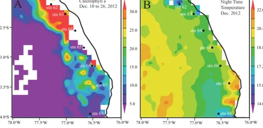
Figure 1. Station map with satellite data from http://disc.sci.gsfc.nasa.gov/giovanni/. (a) sea surface chlorophyllaconcentrations (mg m⁻³), (b) nighttime sea surface temperature (^◦C).

not affected by N-loss (Chang et al., 2010; Bourbonnais et al., 2015).δ¹⁵N biogenic N2was calculated from theδ¹⁵N- N2anomaly as in Bourbonnais et al. (2015). Reproducibility was better than 0.7 µM for excess N₂and 0.03 ‰ forδ¹⁵N- N₂.δ¹⁵N of biogenic N₂was calculated by mass balance as in Bourbonnais et al. (2015).

2.4 Isotope effect (ε)calculations

Isotope effects are estimated using the Rayleigh equations describing the change in isotope ratio as a function of fraction of remaining substrate. The following equations are used for a closed system (Mariotti et al., 1981):

δ¹⁵N−NO⁻₃ =δ¹⁵N−NO⁻₃(f =1)−ε×ln[f1]or (1) δ¹⁵N−DIN=δ¹⁵N−DIN(f=1)−ε×ln[f2], (2) wheref1is the fraction of remaining NO⁻₃ andf2is the fraction of remaining DIN (NO⁻₃+NO⁻₂concentrations).δ¹⁵N- DIN is the average δ¹⁵N for NO⁻₃ and NO⁻₂ weighted by their concentrations. The fraction of remaining DIN is a better estimation of the overall effective isotope effect for N-loss (Bourbonnais et al., 2015), while using NO⁻₃ as the basis to calculateεspecifically targets NO⁻₃ reduction. See below for details off value calculation.

The overall isotope effect for N-loss can also be estimated from theδ¹⁵N of biogenic N₂produced:

δ¹⁵N−biogenic N₂=δ¹⁵N-DIN(f =1)

+ε×f₂/[1−f₂] ×ln[f₂], (3) whereas the closed system equations assume no addition or loss of substrate or product, corresponding steady-state open system equations can account for such effects (Altabet,

2005):

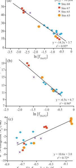
δ¹⁵N−NO⁻₃ =δ¹⁵N−NO⁻₃(f =1)+ε[1−f1]or (4) δ¹⁵N−DIN=δ¹⁵N−DIN(f =1)+ε× [1−f₂] (5) δ¹⁵N−biogenic N₂=δ¹⁵N−DIN(f =1)−ε×f₂. (6) For all equations, the slope representsεand they intercept is the initialδ¹⁵N prior to N-loss. For calculations using Eqs. (3) and (6) we only usedδ¹⁵N values associated with biogenic N₂greater than 7.5 µM because of increasing noise below this level due to the large atmospheric dissolved N₂ background (typically up to∼500 µM).

Since the closed system equations assume no loss or re- supply of substrate or production in a water parcel, they are appropriate where there is little mixing and/or advection is dominant over mixing. The open system equations take into account supply from or loss to surrounding water parcels, e.g.

mixing dominance. Both cases represent extreme situations.

In the next section, we will estimate and compareε using both sets of equations.

To do so, we need to estimate the fraction of NO⁻₃ or DIN remaining (f). The assumption of Redfield stoichiometry (as in Eq. 9) in source waters is typically made:

f_1p= [NO⁻₃]/Np_expectedor (7)

f2p=([NO⁻₃] + [NO⁻₂])/Np_expected (8) Np_expected=15.8·([PO³⁻₄ ] −0.3) (9) N_observed= [NO⁻₃] + [NO⁻₂] + [NH⁺₄], (10) where Np_expected is the concentration expected assuming Redfield stoichiometry. Equation (9) was derived in Chang et al. (2010) from stations to the west of the ETSP ODZ (143–

146^◦W) and takes into account preformed nutrient concentrations. In our study, NH⁺₄ generally did not significantly accumulate, except at station 63, and was thus not included.

(5)

This has been the traditional approach to quantify N-loss in ODZs (N deficit, Np_def), by comparing observed DIN concentrations (N_observed)to Np_expected:

Np_def=Np_expected−N_observed. (11)

However, the assumption of Redfield stoichiometry may not be appropriate in this shallow environment due to prefer- ential release of PO³⁻₄ following iron and manganese oxyhy- droxide dissolution in anoxic sediments (e.g., Noffke et al., 2012). An alternative method of calculatingf makes use of our biogenic N₂measurements to estimate expected N prior to N-loss (N_expected–bio N₂)andf values based on it:

Nexpected−bio N2= [NO⁻₃] + [NO⁻₂] +2× [Biogenic N2] (12) f1bioN₂= [NO⁻₃]/N_expected−bioN₂or (13) f2bioN₂= [NO⁻₃ +NO⁻₂]/N_expected−bio N₂. (14) A third way to estimatefis to use NO⁻₃ or DIN concentrations divided by observed maximum NO⁻₃ or DIN concentrations for the source of the upwelled waters (see red rectangles in Fig. 2).

3 Results

3.1 Hydrographic characterization

During the study period, there was active coastal upwelling especially at station 63 as seen by relatively low satellite sea surface temperatures, higher chlorophyll a concentrations, and a shallow oxycline (Fig. 1). A common relationship and narrow range for T andS were found, compara- ble to T / S signatures for offshore ODZ waters between

∼100 and 200 m depths (Bourbonnais et al. 2015), indicat- ing a common source of water upwelling at these inner shelf stations (Fig. 2). This is expected in these shallow waters, where upwelling of the Peru coastal current with low O₂and high nutrients plays a dominant role (Penven et al., 2005).

O₂ increased only in warmer near-surface waters as a consequence of atmospheric exchange. There was a change in surface water temperature from 15 to 20^◦C (Fig. 1b) with distance along the coast (from 12.0 to 14.0^◦S, about 222 km) that indicates corresponding changes in upwelling intensity.

Stronger local wind forcing likely brought up colder deep water near station 63.

3.2 Dissolved O₂and nutrient concentrations

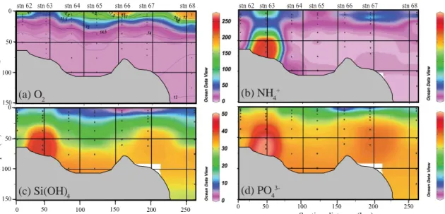
As a consequence of active upwelling sourced from the offshore ODZ, the oxycline was very shallow at our inshore stations. O₂was generally depleted below 10 to 20 m (Fig. 3a) and was always less than 10 µM below 30 m. Be- cause we are focusing on N-transformations that occur in

the absence of O₂, our data analyses will be mainly restricted to samples where O₂ concentration is below this value. Whereas a recent study indicates that denitrification and anammox are reversibly suppressed at nanomolar O₂ levels (Dalsgaard et al., 2014), CTD deployed Seabird O₂ sensors are not sufficiently sensitive to detect such low concentrations and hence our choice of a 10 µM threshold. In contrast, NO⁻₂ oxidation, an aerobic process, was shown to occur even at low to non-detectable O₂(Füssel et al., 2012).

Both Si(OH)₄and PO³⁻₄ concentrations had very similar vertical and along section distributions (Fig. 3c, d). Concen- trations were at a minimum at the surface, presumably due to phytoplankton uptake, and increased with depth to up to 46 and 3.7 µM, respectively. Station 63 had the highest near- bottom concentrations, a likely result of release from the sediments, which is futher supported by high near-bottom NH⁺₄ concentrations (up to∼4 µM) as compared to the other stations (Fig. 3b, c, d).

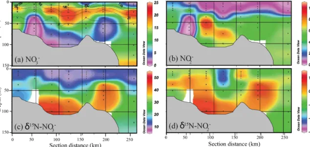
In contrast to other nutrients, NO⁻₃ and NO⁻₂ concentrations were lowest near-bottom at station 63, only reaching their maxima above 60 m. Across most of our stations, NO⁻₃ concentration was 22 µM at 20 to 40 m depth but decreased to near zero deeper within the O₂-depleted zone due to microbially mediated NO⁻₃ reduction (Fig. 4a). NO⁻₂ concentrations correspondingly ranged from 6 to 11 µM for O₂concentrations less than 10 µM (Fig. 4b). The highest NO⁻₂ concentration (11 µM) was found at around 50 m (station 64), but only reached 6 µM at all other stations.

3.3 NO⁻₂ and NO⁻₃ isotope compositions

As a consequence of kinetic isotope fractionation during N- loss, the N and O isotope composition of NO⁻₃ and NO⁻₂ varied inversely with NO⁻₃ and NO⁻₂ concentrations, with max- imumδ¹⁵N andδ¹⁸O values near the bottom at each station.

δ¹⁵N-NO⁻₃ increased from about 10 ‰ in surface waters to up to 50 ‰ in the O2-depleted zone (Fig. 4c), with near bottom values at station 64 significantly higher (50 ‰) than at the other stations which ranged from 20 to 30 ‰ .δ¹⁵N-NO⁻₂ varied from−25 to about 10 ‰ (Fig. 4d), with maximum values also in deeper waters at station 64.

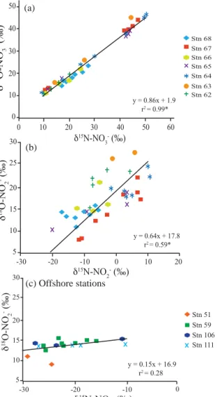
As expected for NO⁻₃ reduction,δ¹⁸O-NO⁻₃ positively co- varied with δ¹⁵N-NO⁻₃ and ranged from 12 to 46 ‰. We observed an overall linear relationship betweenδ¹⁵N-NO⁻₃ and δ¹⁸O-NO⁻₃ with a slope of 0.86, which was significantly different than 1 (p value < 0.05), and a y intercept of 1.90 (r²=0.996, see Fig. 5a). NO⁻₃ δ¹⁵N andδ¹⁸O have been shown to increase equally (ratio 1 : 1) during assimila- tory and dissimilatory NO⁻₃ reduction (Casciotti et al., 2002;

Granger et al., 2004, 2008). However, deviations from this trend have been observed in the ocean and interpreted as evidence for co-occurring NO⁻₃ production processes (Sigman et al., 2005; Casciotti and McIlvin, 2007; Bourbonnais et al., 2009, 2015). In this study, we observed a NO⁻₃δ¹⁸O vs.δ¹⁵N

(6)

Temperature (oC) 18

16

14

12

34.88 34.9 34.92 34.94 34.96 34.98 Salinity [psu]

Oxygen [μM] Nitrite [μM]

(a) (b)

Figure 2. Temperature vs. salinity plots. In (a), color indicates O₂concentration (µM). In (a), color indicates NO⁻₂ concentration (µM).

Black dots in (b) mean no NO⁻₂ concentration data are available. Points in red rectangle at bottom of each plot belong to station 68 for depths greater than 150 m.

(a) O₂ (b) NH₄⁺

(d) PO₄^3- (c) Si(OH)₄

0

50

Depth (m)₁₀₀

150

Section distance (km)

0 100 150 200 250

Depth (m)

0 50 100 150 200 250

stn 62 stn 63 stn 64 stn 65 stn 66 stn 67 stn 68

0

50

100

150

50

Figure 3. O₂and nutrient distribution along the transect. (a) O₂concentration (µM) with isotherm overlay, (b) NH⁺₄ concentration (µM), (c) Si(OH)₄concentration (µM) and (d) PO³⁻₄ concentration (µM). Grey region represents bathymetry. The depth for station 68 is 253 m.

relationship less than 1, likely originating from NO⁻₂ re- oxidation to NO⁻₃ in our environmental setting as in Casciotti and McIlvin (2007). We also observed, for the first time, a significant correlation betweenδ¹⁵N-NO⁻₂ andδ¹⁸O-NO⁻₂ in the ODZ for our in-shore water stations (Fig. 5b). As in prior studies (Casciotti and McIlvin, 2007; Casciotti et al., 2013), no such relationship was observed by us for a nearby set of offshore stations (see Fig. 5c) where longer NO⁻₂ turnover times likely facilitated O isotope exchange with water. We will discuss implications of this unique finding in the next section.

3.4 Theδ¹⁵N difference between NO⁻₃ and NO⁻₂

The difference inδ¹⁵N between NO⁻₃ and NO⁻₂ (1δ¹⁵N) re- flects the combined isotope effects of simultaneous NO⁻₃ reduction, NO⁻₂ reduction, and NO⁻₂ oxidation. For NO⁻₃ reduction alone, highest1δ¹⁵N values would be around 25 ‰ at steady-state (Cline and Kaplan, 1975; Brandes et al., 1998;

Voss et al., 2001; Granger et al., 2004, 2008). The effect of NO⁻₂ reduction would be to increase theδ¹⁵N of the residual NO⁻₂, thus decreasing1δ¹⁵N. In contrast, NO⁻₂ oxidation is associated with an inverse kinetic isotope effect (Cas- ciotti, 2009) which acts to decrease the residualδ¹⁵N of NO⁻₂

(7)

Figure 4. Transects off the Peru coast for (a) NO⁻₃ concentration (µM) with O₂overlay, (b) NO⁻₂ concentration (µM), (c)δ¹⁵N-NO⁻₃ (‰) and (d)δ¹⁵N-NO⁻₂ (‰). Gray region represents approximate bathymetry. No isotopic data are available for the deeper samples collected at station 63, because NO⁻₃ and NO⁻₂ concentrations were below analytical limits (< 0.5 µM).

and hence overall increases the1δ¹⁵N. Therefore, following NO⁻₂ oxidation, 1δ¹⁵N may be larger than expected from NO⁻₃ and NO⁻₂ reduction alone, especially if the system is not at steady-state (Casciotti et al., 2013). 1δ¹⁵N ranged from 15 to 40 ‰ (average=29.78 ‰ and median=32.5 ‰) for samples with O₂< 10 µM. These results confirm the presence of NO⁻₂ oxidation for at least some of our depth inter- vals.

3.5 N deficit, biogenic N₂andδ¹⁵N-N₂

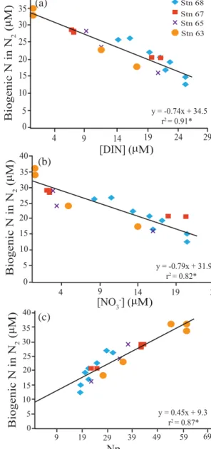
N deficits, biogenic N2concentrations, andδ¹⁵N-N2anoma- lies relative to equilibrium with atmosphere were overall greater in the O₂-depleted zone reaching highest values near the bottom of station 63 (Fig. 7). N deficit, calculated assuming Redfield stoichiometry (Eqs. 9 to 11), ranged from 17 to 59 µM in this region. The concentration of biogenic N in N₂ ranged from 12 to 36 µM-N and, as expected, was strongly linearly correlated with N deficit (r²=0.87; Fig. 8c). How- ever, the slope of 0.45 for the linear relationship shows biogenic N in N₂ to be only half that expected from Np_def, a possible consequence of benthic PO³⁻₄ release. The linear relationship (r²=0.91) observed between biogenic N in N₂ and DIN (Fig. 8a) supports a single initial DIN value for the source waters to our stations and hence validates using this as a basis for calculating f. The slope of the correlation (0.74) is much closer to 1 as compared to the correlation with Np_def, further supporting excess PO⁻³₄ as a contributor to the latter. However this value is still significantly less than 1, suggesting that biogenic N in N₂ may also be underesti- mated. Because our data are restricted to O₂-depleted depths, it is unlikely that biogenic N₂was lost to the atmosphere. Al-

ternatively, mixing of water varying in N₂/Ar can result in such underestimates of biogenic N₂ when N₂/Ar anomalies are used to calculate excess N₂(see Charoenpong et al., 2014). As seen below, our estimates ofεare rather insensitive to choice of Np_def, biogenic N in N₂, or DIN concentration changes as the basis for calculation off.

The δ¹⁵N-N2 anomaly, i.e., the difference between the δ¹⁵N-N2observed and at equilibrium, derived as in Charoen- pong et al. (2014), ranged from −0.2 to 0.1 ‰ (Fig. 7c).

The corresponding range inδ¹⁵N biogenic N2at O2< 10 µM was from−9.0 to 3.2 ‰. Negative δ¹⁵N-N2 anomaly (i.e., lowerδ¹⁵N-biogenic N₂)is produced at the onset of N-loss, because extremely depleted¹⁵N-N₂ is first produced. At a more advanced N-loss stage, we expect δ¹⁵N-N₂ anomaly andδ¹⁵N-biogenic N₂to increase, which we observed in this study, as heavier¹⁵N is added to the biogenic N₂pool. The δ¹⁵N-N₂ anomaly signal appears small when compared to the isotopic composition of NO⁻₃ and NO⁻₂ but is (1) ana- lytically significant and (2) the result of dilution by the large background of atmospheric N₂(400 to 500 µM N₂).

3.6 Isotope effect (ε)

Isotope effects were calculated using Eqs. (1) to (6) to compare closed vs. open system assumptions as well as different approaches to estimatingf. Examples of plots of the closed system equations withf calculated using biogenic N₂, are shown in Fig. 6. Comparison of results using all three approaches for calculatingf (i.e. Redfield stoichiometry, biogenic N₂and observed substrate divided by maximum “upwelled” concentration, (see Sect. 2.4)) are shown in Table 1 (closed system) and 2 (open system). In the case of the closed

(8)

30

δ18O-NO2- (‰)

25

20 15 10 5

δ¹⁵N-NO₂^- (‰)^-10

-20 -30

Stn 51 Stn 59 Stn 106 Stn 111

(c) Offshore stations 50

δ18O-NO3- (‰)

δ¹⁵N-NO₃^- (‰) 40

30 20 10 0

50

30 60

20 10 0

Stn 68 Stn 67 Stn 66 Stn 65 Stn 64 Stn 63 Stn 62

40 30

δ18O-NO2- (‰)

δ¹⁵N-NO₂^- (‰) 25

20 15 10 5

10

0 20

-10 -20 -30

(a)

(b)

y = 0.64x + 17.8 r²= 0.59*

y = 0.86x + 1.9 r²= 0.99*

0 y = 0.15x + 16.9 r²= 0.28

Figure 5. Relationships between δ¹⁵N and δ¹⁸O for NO⁻₃ and NO⁻₂, respectively, for O₂≤10 µM. (a)δ¹⁸O-NO⁻₃ vs.δ¹⁵N-NO⁻₃ for station 62 to 68. (b)δ¹⁸O-NO⁻₂ vs.δ¹⁵N-NO⁻₂ for station 62 to 68. (c)δ¹⁸O-NO⁻₂ vs.δ¹⁵N-NO⁻₂ for M90 offshore stations 51, 59, 106 and 111 (see text, Sect. 3.3). For each plot, overall linear regressions are shown. Significant correlation coefficients at a 0.05 significance level are denoted by *.

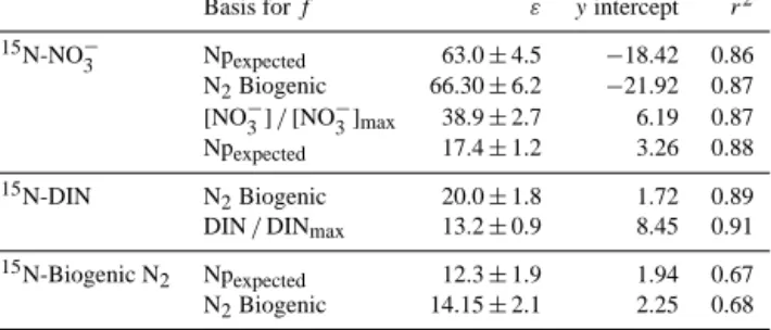
system,εvalues were in all cases lower than canonical ones, ranging narrowly from∼6 ‰ for changes in theδ¹⁵N of DIN to∼14 ‰ for changes inδ¹⁵N-NO⁻₃ (Table 1). For the open system equations, estimatedεwas higher and covered a large and unrealistic range from∼12 ‰ for changes in the biogenic N₂ to∼63 ‰ for changes in the δ¹⁵N of NO⁻₃. For our inshore water stations, where we observed a single water mass (Fig. 2), a closed system should be a more realistic approximation of ε. The Rayleigh equations’ y intercepts, wheref =1, represent the initialδ¹⁵N of NO⁻₃ or DIN, and varied from −0.5 to 10.9 and −21.9 to 8.5 ‰ for closed and open systems, respectively. The higher end of this range

Table 1.εfor NO⁻₃ reduction and net N loss estimated from both DIN consumption and produced biogenic N₂using Rayleigh closed system equations (Eqs. 1–3). Results are calculated forf based on either Np_expected (Eqs. 7–9), biogenic N₂(Eqs. 12–14) and measured substrate divided by maximum (upwelled) substrate concentrations (see text, Sect. 2.4). The standard error of the slope (ε)is shown.

Basis forf ε yintercept r²

δ¹⁵N-NO⁻₃ Npexpected 13.9±0.7 3.74 0.92

N2Biogenic 14.3±0.9 3.71 0.95 [NO⁻₃]/[NO⁻₃]max 14.7±0.6 −0.55 0.95 δ¹⁵N-DIN Npexpected 6.3±0.3 7.20 0.92 N2Biogenic 6.6±0.4 6.71 0.94 DIN/DINmax 7.4±0.6 10.90 0.91 δ¹⁵N-Biogenic N₂ Np_expected 10.5±1.5 2.94 0.70 N₂Biogenic 10.6±1.5 3.04 0.72

is more realistic based on prior isotopic measurements for source waters (e.g., Bourbonnais et al., 2015).

4 Discussion

4.1 Behavior of NO⁻₂

NO⁻₂ is an important intermediate during either oxidative or reductive N-cycle pathways and can accumulate at relatively high concentrations through the ocean. While NO⁻₂ is generally elevated at the base of the sunlit euphotic zone (i.e. primary NO⁻₂ maximum; Dore and Karl, 1996; Lomas and Lip- schultz, 2006), highest concentrations are found in ODZ’s as part of the secondary NO⁻₂ maximum (Codispoti and Chris- tensen 1985; Lam et al., 2011). Accordingly, high NO⁻₂ concentrations ranging from 7.2 to 10.7 µM were observed at 50–75 m depth in coastal O2-depleted waters in this study as a likely consequence of dissimilatory NO⁻₃ reduction (e.g., Lipschultz et al., 1990; Lam et al., 2009; Kalvelage et al., 2013).

To assess the influence of the various N cycle processes that have NO⁻₂ as either a substrate or product, we first ex- amined the relationship between theδ¹⁵N andδ¹⁸O of NO⁻₂. Several processes can influence the isotopic composition of NO⁻₂. NO⁻₃ reduction to NO⁻₂ is associated with aε of 20 to 30 ‰ (Cline and Kaplan, 1975; Brandes et al., 1998; Voss et al., 2001; Granger et al., 2004, 2008) and acts to produce NO⁻₂ depleted in¹⁵N and¹⁸O. In contrast, NO⁻₂ reduction as part of either anammox, denitrification or DNRA increases both theδ¹⁵N and δ¹⁸O of residual NO⁻₂, with laboratory and field estimates forεclustering around 12 to 16 ‰ (Bryan et al., 1983; Brunner et al., 2013; Bourbonnais et al., 2015).

However, NO⁻₂ oxidation to NO⁻₃ at low or non-detectable O₂has been shown to be an important sink for NO⁻₂ in ODZs (e.g. Füssel et al., 2012). Anammox bacteria can also use

(9)

4

δ15N-biogenic N2 (‰) ²₀

-8

f_2bioN2/[1-f_2bioN2^-0.5] × ln [f_2bioN2]

-0.9

(c) δ15N-NO3- (‰)

ln [f_1bioN2] 40

30 20 10 0

-1.0

-2.0 -0.5

-2.5 -3.0 -3.5

-1.5

δ15N-DIN (‰)

ln [f_2bioN2]

19

13 11 9 7

-0.5

-1.0 0

-1.5 -2.0 -2.5

(a)

(b)

y = -14.3x + 3.7 r²= 0.95*

50 60

0

[O₂] < 10 μM

15 17

y = -6.5x + 6.7 r²= 0.94*

-2 -4 -6

-10

-0.7 -0.3 -0.1

y = 10.6x + 3.0 r²= 0.72*

Figure 6. Raleigh relationships used to estimateε(slope) and initial δ¹⁵N-substrate (yintercept) assuming a closed system. (a) for NO⁻₃ reduction (Eq. 1 and text, Sect. 2.4), (b) for N-loss calculated from the substrate (DIN) consumption (Eq. 2 and text, Sect. 2.4) and (c) for N-loss calculated from theδ¹⁵N of biogenic N₂(Eq. 3 and text, Sect. 2.4). In (c), only samples with O₂ concentrations less than 10 µM and biogenic N₂values > 7.5 µM were considered. Signifi- cant correlation coefficients at a 0.05 significance level are denoted by *.

NO⁻₂ as an electron donor during CO₂fixation under anaerobic conditions (Strous et al., 2006).

Nitrite oxidation has its own unique set of isotope effects (Casciotti, 2009; Buchwald and Casciotti, 2010). Nitrite oxidation incurs an unusual inverse N isotope effect varying from−13 ‰ for aerobic (Casciotti, 2009) to−30 ‰ for anammox-mediated NO⁻₂ oxidation (Brunner et al., 2013), resulting in lowerδ¹⁵N for NO⁻₂ as it is oxidized to NO⁻₃, and increasing 1δ¹⁵N. Moreover, enzyme catalysis associated with NO⁻₂ oxidation is readily reversible (Friedman et

0

50

Depth (m) ₁₀₀

1500

50

Depth (m)₁₀₀

1500

50

Depth (m)₁₀₀

150

0 50 100 150 200 250

(a) Np_def

(c) δ¹⁵N-N anomaly₂ (b) Biogenic N in N₂

Figure 7. N deficit, biogenic N in N₂andδ¹⁵N-N₂anomaly with O₂overlaid. (a) N deficit calculated using PO³⁻₄ (µM) (Np_def)and assuming Redfield stoichiometry (see Eqs. 9, 10 and 11, Sect. 2.4).

(b) biogenic N in N₂(µM). (c)δ¹⁵N-N₂anomaly relative to equilibrium with atmosphere (‰). Biogenic N₂orδ¹⁵N-N₂ anomaly were not measured at stations 62, 64 and 66.

al., 1986) also causing O isotope exchange between NO⁻₂ and water (Casciotti et al., 2007). O atom incorporation during both NH⁺₄ and NO⁻₂ oxidation have also been shown to occur with significant isotope effect, such that theδ¹⁸O of newly microbially produced NO⁻₃ in the ocean range from

−1.5 to 1.3 ‰ (Buchwald and Casciotti, 2012).

Past studies have found NO⁻₂δ¹⁸O values in ODZ’s in isotope equilibrium with water as a likely consequence of relatively long turnover time (e.g., Buchwald and Casciotti, 2013; Bourbonnais et al., 2015). O isotope exchange involves the protonated form, HNO₂, but because of its high pKa as compared to NO⁻₃, this process can occur even at neutral to alkaline ocean pH on a timescale of 2 to 3 months at en- vironmentally relevant temperatures (Casciotti et al., 2007).

NO⁻₂δ¹⁸O isotopic composition at equilibrium with water is a function of theδ¹⁸O of water and temperature (+14 ‰ for seawater at 22^◦C) (Casciotti et al., 2007; Buchwald and Cas- ciotti, 2013) and is independent of itsδ¹⁵N value such that plots of NO⁻₂δ¹⁸O vs.δ¹⁵N usually have a slope of near zero.

This is seen in our NO⁻₂ data from offshore stations occupied during M90 (Fig. 5c).

(10)

We observed, for the first time, a significant linear relationship for NO⁻₂δ¹⁸O vs. δ¹⁵N at our inshore stations (slope=0.64±0.07,r²=0.59,p value=3×10⁻⁶)where O₂< 10 µM (Fig. 5b). Coupled δ¹⁵N and δ¹⁸O effects for NO⁻₂ have not been as well studied as NO⁻₃. Nevertheless, if NO⁻₂ turnover was faster than equilibration time with water, NO⁻₃ and NO⁻₂ reduction whether as part of the denitrification, anammox or DNRA pathways, should also produce a positive relationship between NO⁻₂δ¹⁵N andδ¹⁸O. In contrast to our offshore stations (Fig. 5c), this positive relationship thus demonstrates that the oxygen isotopic composition of NO⁻₂ is not in equilibrium with water due to both rapid NO⁻₂ turnover and the dominance of NO⁻₂ reduction over oxidation in Peru coastal waters. Higher rates for aerobic NH⁺₄ and NO⁻₂ oxidation, as well as anaerobic NO⁻₃ reduction to NO⁻₂, and further reduction to NH⁺₄ (DNRA) or N2, have been reported in shallow waters off Peru presumably due to increased coastal primary production and organic matter supply to the in-shore OMZ (e.g. Codispoti et al., 1986; Lam et al., 2011; Kalvelage et al., 2013). However, as our observations are restricted to anoxic waters, only high rates of N-loss could explain this more rapid NO⁻₂ turnover.

In principal, we can estimate NO⁻₂ turnover time from knowledge of rates for exchange with water and assumptions of the δ¹⁸O vs. δ¹⁵N slope expected in the absence of exchange. Unfortunately, the slope of the relationship between NO⁻₂δ¹⁸O vs.δ¹⁵N expected in the absence of equilibration with water is not yet known. An upper limit for turnover time for NO⁻₂ can be estimated based on equilibration time as a function of in situ pH and temperature (Buchwald and Cas- ciotti, 2013). During the M91 cruise in December, subsurface temperature was 13 to 15^◦C along our transect and corresponding pH was near 7.8 (Michelle Graco, unpublished data). Assuming the NO⁻₂ pool is in steady-state, we estimated an equilibration time of up to∼40 days for pH near 7.8 (estimated from equation 1 and Fig. 2 in Buchwald and Casciotti, 2013). A turnover time of up to 40 days implies a flux of N through the NO⁻₂ pool of at least 0.21 µM d⁻¹, as estimated from the maximum NO⁻₂ concentration observed in this study divided by this estimated turnover time. As- suming steady-state, this range also approximates the rates of NO⁻₃ reduction as well as NO⁻₂ oxidation plus production of N2from NO⁻₂. This estimated flux is consistent with measured high NO⁻₃ reduction and NO⁻₂ oxidation rates of up to

∼1 µM d⁻¹in Peru coastal waters (< 600 m depth, Kalvelage et al., 2013).

NO⁻₂ oxidation is a chemoautotrophic process that re- quires a thermodynamically favorable electron acceptor such as O2. As mentioned above, NO⁻₂ oxidation appears to occur in ODZ’s at low or non-detectable O2 (e.g. Füssel et al., 2012) despite lack of knowledge of its thermodynamically favorable redox couple. The difference in δ¹⁵N between NO⁻₂ and NO⁻₃ (1δ¹⁵N =δ¹⁵N-NO⁻₃ −δ¹⁵N-NO⁻₂

40 35 30

5

Np_def (c)

Biogenic N in N2 (

μ M) 25 20 15

5

0 4 9 14 19 24

[NO₃^-] (μM)

35

15 10 5 0

19

14 24

4 9

(a)

(b)

y = -0.74x + 34.5 r²= 0.91*

30 40

29

20

y = -0.79x + 31.9 r²= 0.82*

25 20 15

0 9

y = 0.45x + 9.3 r²= 0.87*

10 35

25 30 40

Biogenic N in N2 (

μ M)

10

19 29 39 49 59 69

Biogenic N in N2 (

μ M)

[DIN] (μM)

Figure 8. Cross-plots of biogenic N in N₂vs. DIN (a), NO⁻₃ (b) and Np_def(c), see Eqs. (9–11) in text). All plots have the overall linear regression overlaid. All the points are restricted to O₂concentrations less than 10 µM. Biogenic N₂was not measured for stations 62, 64 and 66. Significant correlation coefficients at a 0.05 significance level are denoted by *.

see Sect. 3.3) is further evidence for the presence of NO⁻₂ oxidation in the ODZ (e.g. Casciotti et al., 2013). At steady- state, and in the absence of NO⁻₂ oxidation,1δ¹⁵N should be no more than theεfor NO⁻₃ reduction (20 to 30 ‰) mi- nus the ε for NO⁻₂ reduction by denitrifying or anammox bacteria (12–16 ‰; Bryan et al., 1983; Brunner et al., 2013;

Bourbonnais et al., 2015) or 8–18 ‰ . Our results range from 15–40 ‰ and average 29.8 ‰ for samples with O₂concentrations < 10 µM.