www.biogeosciences.net/14/2167/2017/
doi:10.5194/bg-14-2167-2017
© Author(s) 2017. CC Attribution 3.0 License.
Upwelling and isolation in oxygen-depleted anticyclonic modewater eddies and implications for nitrate cycling
Johannes Karstensen1, Florian Schütte1, Alice Pietri2, Gerd Krahmann1, Björn Fiedler1, Damian Grundle1, Helena Hauss1, Arne Körtzinger1,3, Carolin R. Löscher1,a, Pierre Testor2, Nuno Vieira4, and Martin Visbeck1,3
1GEOMAR, Helmholtz Zentrum für Ozeanforschung Kiel, Düsternbrooker Weg 20, 24105 Kiel, Germany
2Sorbonne Universites (UPMC Univ. Pierre et Marie Curie, Paris 06)-CNRS-IRD-MNHN, UMR 7159, Laboratoire d’Oceanographie et de Climatologie (LOCEAN), Institut Pierre Simon Laplace (IPSL), Observatoire Ecce Terra, 4 place Jussieu, 75005 Paris, France
3Kiel University, Kiel, Germany
4Instituto Nacional de Desenvolvimento das Pescas (INDP), Cova de Inglesa, Mindelo, São Vicente, Cabo Verde
anow at: Nordic Center for Earth Evolution, University of Southern Denmark, Campusvej 555230 Odense M, Denmark Correspondence to:Johannes Karstensen (jkarstensen@geomar.de)
Received: 28 February 2016 – Discussion started: 11 March 2016
Revised: 7 March 2017 – Accepted: 31 March 2017 – Published: 27 April 2017
Abstract. The temporal evolution of the physical and bio- geochemical structure of an oxygen-depleted anticyclonic modewater eddy is investigated over a 2-month period using high-resolution glider and ship data. A weakly stratified eddy core (squared buoyancy frequencyN2∼0.1×10⁻⁴s−2)at shallow depth is identified with a horizontal extent of about 70 km and bounded by maxima inN2. The upperN2maxi- mum (3–5×10⁻⁴s−2)coincides with the mixed layer base and the lower N2 maximum (0.4×10⁻⁴s−2) is found at about 200 m depth in the eddy centre. The eddy core shows a constant slope in temperature/salinity (T /S) characteristic over the 2 months, but an erosion of the core progressively narrows down the T /S range. The eddy minimal oxygen concentrations decreased by about 5 µmol kg−1in 2 months, confirming earlier estimates of oxygen consumption rates in these eddies.
Separating the mesoscale and perturbation flow compo- nents reveals oscillating velocity finestructure (∼0.1 m s−1) underneath the eddy and at its flanks. The velocity finestruc- ture is organized in layers that align with layers in properties (salinity, temperature) but mostly cross through surfaces of constant density. The largest magnitude in velocity finestruc- ture is seen between the surface and 140 m just outside the maximum mesoscale flow but also in a layer underneath the eddy centre, between 250 and 450 m. For both regions a cy- clonic rotation of the velocity finestructure with depth sug-
gests the vertical propagation of near-inertial wave (NIW) energy. Modification of the planetary vorticity by anticy- clonic (eddy core) and cyclonic (eddy periphery) relative vor- ticity is most likely impacting the NIW energy propagation.
Below the low oxygen core salt-finger type double diffusive layers are found that align with the velocity finestructure.
Apparent oxygen utilization (AOU) versus dissolved in- organic nitrate (NO−3) ratios are about twice as high (16) in the eddy core compared to surrounding waters (8.1). A large NO−3 deficit of 4 to 6 µmol kg−1 is determined, ren- dering denitrification an unlikely explanation. Here it is hy- pothesized that the differences in local recycling of nitrogen and oxygen, as a result of the eddy dynamics, cause the shift in the AOU : NO−3 ratio. High NO−3 and low oxygen waters are eroded by mixing from the eddy core and entrain into the mixed layer. The nitrogen is reintroduced into the core by gravitational settling of particulate matter out of the eu- photic zone. The low oxygen water equilibrates in the mixed layer by air–sea gas exchange and does not participate in the gravitational sinking. Finally we propose a mesoscale–
submesoscale interaction concept where wind energy, medi- ated via NIWs, drives nutrient supply to the euphotic zone and drives extraordinary blooms in anticyclonic mode-water eddies.
1 Introduction
Eddies are associated with a wide spectrum of dynamical processes operating on mesoscale (order 100 km) and sub- mesoscale (order of 0.1 to 10 km) horizontal scales, but also down to the molecular scale of three-dimensional turbulence (McWilliams, 2016). The interaction of these processes cre- ates transport patterns in and around eddies that provoke often very intense biogeochemical and biological feedback such as plankton blooms (Lévy et al., 2012; Chelton et al., 2011).
The simplest way of classifying eddies is by their sense of rotation into cyclonic-rotating and anticyclonic-rotating ed- dies (e.g. Chelton et al., 2011; Zhang et al., 2013). How- ever, when considering the vertical stratification of eddies, a third group emerges that shows in a certain depth range a downward displacement of isopycnals towards the eddy cen- tre, as observed in anticyclonic eddies (ACEs), but an up- ward displacement of isopycnals in a depth range above, as observed in cyclonic eddies (CEs). Because the depth inter- val between upward and downward displaced isopycnals cre- ates a volume of homogenous properties, called a “mode”, such hybrid eddies have been called anticyclonic modewater eddies (ACMEs) or intra-thermocline eddies (McWilliams, 1985; D’Asaro, 1988; Kostianoy and Belkin, 1989; Thomas, 2008). Modewater eddies occur not only in the thermo- cline, but also in the deep ocean, like for example Mediter- ranean Outflow lenses (Meddies) in the North Atlantic (Armi and Zenk, 1984) or those associated with deep convection processes (e.g. the Mediterranean Sea, Testor and Gascard, 2006). Schütte et al. (2016a, b) studied eddy occurrence in the thermocline of the tropical eastern North Atlantic con- sidering CEs, ACEs, and ACMEs. They estimated that about 9 % of all eddies (20 % of all anticyclonic-rotating eddies) in the eastern tropical North Atlantic are ACMEs. Zhang et al. (2017) found modewater eddies in all ocean basins and primarily in the upper 1000 m.
More than a decade ago a dedicated observational pro- gramme was carried out in the Sargasso Sea in the western North Atlantic in order to better understand the physical–biogeochemical interactions in mesoscale eddies.
The studies revealed that in ACMEs particularly intense deep chlorophyll a layers are found which align with a maximum concentration of diatoms and maximum pro- ductivity (McGillicuddy et al., 2007). The high productiv- ity was explained by the “eddy–wind interaction” concept (McGillicuddy et al., 2007, going back to a work by Dewar and Flierl, 1987) based on an Ekman divergence that is gener- ated from the horizontal gradient in wind stress across anticy- clonic rotating eddies. While the productivity is evident from observations, the concept was questioned (Mahadevan et al., 2008). High-resolution ocean model simulations, comparing runs with or without eddy–wind interaction, reproduced only a marginal impact on ocean productivity (but a strong impact on physics; Eden and Dietze, 2009). A tracer release exper-
iment within an ACME revealed a vertical flux in the order of magnitude (several metres per day) as calculated based on the eddy–wind interaction concept (Ledwell et al., 2008).
Levy et al. (2012) summarized the submesoscale up- welling at fronts in general, not specifically for mesoscale eddies, and the impact on oceanic productivity. A key role is played by the vertical flux of nutrients into the euphotic zone, either by advection along outcropping isopycnals or by mixing. Moreover, eddies are retention regions (d’Ovidio et al., 2013) and the upwelled nutrients are kept in the eddy and utilized for new production (Condie and Condie, 2016).
In the tropical eastern North Atlantic ACMEs with very low oxygen concentrations in their cores have been observed (Karstensen et al., 2015). The generation of the low oxygen concentrations was linked to upwelling of nutrients and high productivity in the euphotic zone of the eddy followed by a remineralization of the sinking organic matter and accompa- nied by respiration. The temperature and salinity character- istics of the eddy core were found unaltered even after many months of westward propagation of ACMEs, indicating a well-isolated core. It was surprising to find a well-isolated eddy core, while in parallel an enhanced vertical nutrient flux is required to maintain the high productivity in the eddy.
A measure of the importance of local rotational effect rel- ative to the Earth’s rotation is given by the Rossby number defined asRo= ζ
f, and where ζ =∂v
∂x−∂v
∂y is the vertical component of the relative vorticity (u andv are zonal and meridional velocities, respectively) andf the planetary vor- ticity. Planetary flows have smallRo, say up to ∼0.2, but local rotational effects gain importance withRoapproaching 1, for example in eddies and fronts.
The horizontal velocity shear of mesoscale eddies creates a negative (positive)ζ in anticyclonic (cyclonic) rotating ed- dies. Theζ modifiesf to an “effective planetary vorticity”
(feff=f+ζ
2)(Kunze, 1985; Lee and Niiler, 1998). Nega- tive ζ of anticyclonic-rotating eddies results in a feff< f in their cores. In the region outward from the maximum swirl velocity of an anticyclonic eddy, towards the surround- ing waters, a positive ζ “ridge” is created where feff> f (e.g. Halle and Pinkel, 2003). The local modification of f has implications for the propagation of near-inertial inter- nal waves (NIWs): in the core of an anticyclonic-rotating eddy (feff> f )the NIW become superinertial and their ver- tical propagation speed increases (Kunze et al., 1995). In the ridge region of any anticyclonic-rotating eddy the NIWs ex- perience a reduction in vertical speed, and they may reflect becausefeff< f. Downward propagation of NIWs may re- sult in an accumulation of wave energy at some critical depth and eventually part of the energy is dissipated by buoyancy release through vertical mixing (Kunze, 1985; Kunze et al., 1995; Whitt and Thomas, 2013; Whitt et al., 2014).
In anticyclonic-rotating eddies the downward propagation of wave energy in thefeff< f region has been observed and modelled (Kunze, 1985; Gregg et al., 1986; Lee and Niiler, 1998; Koszalka et al., 2010; Joyce et al., 2013; Alford et al.,
2016). Lee and Niiler (1998) simulated the NIW interaction with eddies (ACEs, CEs, ACMEs) and found vertical propa- gation of the NIW energy, the “inertial chimney”. In the case of an ACME with a low squared buoyancy frequency (N2) layer they report on NIW energy accumulating below the eddy core and not inside as seen for ACEs. This change in en- ergy accumulation was attributed to the vertical stratification of the ACME, in particular the twoN2maxima that shield the low stratified eddy core. Kunze et al. (1995) analysed NIW energy propagation in an ACE. Within a critical layer at the inner sides of the ACE and where thefeff increases are≥1, the vertical propagation of NIWs is hampered, and energy accumulates, the bulk is released by turbulent mixing.
The vertical shear of the horizontal velocity that is gener- ated by NIWs can eventually force overturning e.g. when ap- proaching a critical layer (Kunze et al., 1995). The tendency of a stratified water column to become unstable through ve- locity shearS=
r ∂u
∂z
2
+
∂v
∂z
2
can be estimated from the gradient Richardson number Ri=N2/S2. A Ri<1/4 has been found to be a necessary condition for the shear to over- come the stratification and to generate overturning. However, Whitt et al. (2014) measured enhanced dissipation was with shear probes along the Gulf Stream front in several regions where NIW shear producedRi<1.
Recent observational studies using microstructure shear probe data report enhanced mixing in a narrow depth range of a local, verticalN2maximum, above and below the low stratified ACME core (Sheen et al., 2015; Kawaguchi et al., 2016). By applying an internal wave ray model to the N2 stability profile and vertical shear profile from outside and from inside of an ACME, Sheen et al. (2015) could show that only a very limited range of incident angles of inter- nal waves could propagate into the eddy core. Most NIWs encounter a critical layer above and below the eddy, in the regions where they observed enhanced mixing. Halle and Pinkel (2003) analysed NIW interaction with eddies having an ACME-like vertical structure in the Arctic and explained the low internal wave activity in the core as the result of an increase (order of magnitude) in wave group speed caused by low N2 accompanied by lowering of wave energy density.
Krahmann et al. (2008) reported observations of enhanced NIW energy in the vicinity of a Meddie. Meddie signatures of thermohaline layering at the eddy periphery have often been observed together with the occurrence of critical lay- ers that support the energy transfer from the mesoscale to the submesoscale (Hua et al., 2013).
In this paper we investigate the hydrography, currents, and biogeochemical characteristics of a low oxygen ACME and its temporal evolution. High-resolution underwater glider and ship data allow us to describe the eddy structure at sub- mesoscale resolution. Characteristics of a low oxygen ACME found in the eastern tropical North Atlantic are provided. The paper is part of a series of publications that report on differ-
ent genomic, biological, and biogeochemical aspects of this eddy (Löscher et al., 2015; Hauss et al., 2016; Fiedler et al., 2016; Schütte et al., 2016b).
2 Data and methods
Targeted eddy surveys are logistically challenging. Eddy locations can be identified using real-time satellite SLA data. To further differentiate a positive SLA (indicative of anticyclonic-rotating eddies) into either an ACE or an ACME the SST anomaly across the eddy was additionally inspected, because ACMEs (ACEs) in the eastern tropical North At- lantic show a cold (warm) SST anomaly (Schütte et al., 2016a, b). For further evidence, Argo profile data were in- spected to detect anomalously low temperature/salinity sig- natures also indicative of low oxygen ACMEs in the region (Karstensen et al., 2015; Schütte et al., 2016b). In late De- cember 2013 a candidate eddy was identified through this mechanism and in late January 2014 a pre-survey was initi- ated, making use of autonomous gliders. After confirmation that the candidate eddy was indeed a low oxygen ACME, two ship surveys (ISL_00314, M105; Fiedler et al., 2016) and further glider surveys followed.
2.1 Glider surveys
Data from glider IFM12 and glider IFM13 were used in this study (Fig. 1). Glider IFM12 surveyed temperature, salinity, and oxygen to a depth of 500 m as well as chlorophyllaflu- orescence and turbidity to 200 m depth. Glider IFM13 sur- veyed temperature, salinity, and oxygen to a depth of 700 m as well as chlorophyllafluorescence and turbidity to 200 m depth. Glider IFM13 was also equipped with a nitrate sensor that sampled to 700 m depth.
For one full eddy survey of glider IFM12 (Fig. 1) we com- bined data from 3 to 5 February and from 7 to 10 Febru- ary 2014 because, due to technical problems, data were not recorded in between these periods. Glider IFM13 surveyed one full eddy section from 3 to 7 April 2014. All glider data were internally recorded as a time series along the flight path, while for the analysis the data were linearly interpolated onto a regular pressure grid of 1 dbar resolution. For the purposes of this study we consider the originally slanted profiles as vertical profiles.
2.2 Glider sensor calibrations
Both gliders were equipped with a pumped CTD (conductiv- ity, temperature, and depth) and no evidence for further time lag correction of the conductivity sensor was found. Oxygen was recorded with AADI Aanderaa optodes (model 3830).
The optodes were calibrated in reference to SeaBird SBE43 sensors mounted on a regular ship-based CTD, which in turn were calibrated using Winkler titration of water samples (see Hahn et al., 2014). Considering the full oxygen range, a root
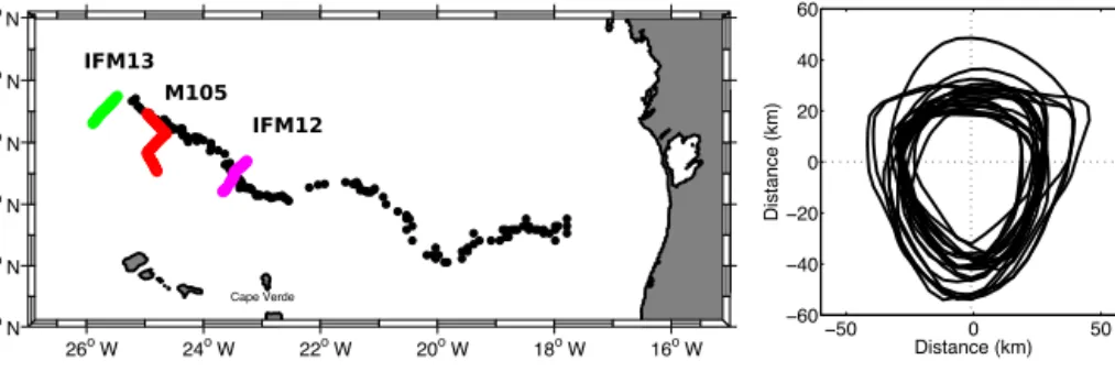
Figure 1. (a)Positions of the glider IFM12 (magenta) and IFM13 (green) surveys and the M105 ship survey (red dots). The Mauritanian coast is in the east, the Cape Verde Islands in the south. The black dots represent the sea level anomaly (SLA) based estimate of the eddy trajectory (see e.g. Fiedler et al., 2016).(b)Last closed geostrophic contours from SLA analysis during the IMF12 survey projected on the eddy centre.
mean square (rms) error of 3 µmol kg−1is found. However, for calibrating at the chemically forced 0 µmol kg−1oxygen, the rms error is smaller and about 1 µmol kg−1. The calibra- tion process also removes a large part of the effects of the slow optode response time via a reverse exponential filter (time constants were 21 and 23 s for IFM12 and IFM13, re- spectively). As there remained some spurious difference be- tween down and up profiles we averaged upcast and down- cast profiles to further minimize the slow sensor response problem in high gradient regions, particularly at the mixed layer base. The optical (Wetlabs ECO-PUC) chlorophyll a fluorescence and turbidity data were not calibrated against bottle samples; only the factory calibration is applied. We subtracted a dark (black tape on sensor) offset value and the data are given here in relative units.
The nitrate (NO−3)measurements on glider IFM13 were collected using a Satlantic Deep SUNA sensor. The SUNA emits light pulses and measures spectra in the ultraviolet range of the electromagnetic spectrum. It derives the NO−3 concentration from the concentration-dependent absorption over a 1 cm long path through the sampled seawater. Dur- ing the descents of the glider the sensor was programmed to collect bursts of five measurements every 20 s or about ev- ery 4 m in the upper 200 m and every 100 s or about every 20 m below 200 m. The sensor had been factory calibrated 8 months prior to the deployment. The spectral measure- ments of the SUNA were post-processed using Satlantic’s SUNACom software, which implements a temperature and salinity dependent correction to the absorption (Sakamoto et al., 2009). The SUNA sensors’ light source is subject to aging which results in an offset NO−3 concentration (Johnson et al., 2013). To determine the resulting offset, NO−3 concentrations measured on bottle samples by the standard wet-chemical method were compared against the SUNA-based concentra- tions. The glider recorded profiles close to the CVOO moor- ing observatory (see Fiedler et al., 2016) at the beginning and end of the mission. These were compared to the mean concentrations of ship samples taken in the vicinity of the
CVOO location (Fiedler et al., 2016). In addition we com- pared glider measurements within the ACME to NO−3 sam- ples from the ship surveys performed during the eddy experi- ment (see Löscher et al., 2015; Fiedler et al., 2016). The com- parison showed on average no offset (0.0±0.2 µmol kg−1).
However, near the surface the bottle measurements indicated NO−3 concentrations below 0.2 µmol kg−1 at CVOO, while the SUNA delivered values of about 1.8 µmol kg−1possibly related to technical problems near the surface. We thus es- timate the accuracy of the NO−3 measurements to be better than 2.5 µmol kg−1with a precision of each value of about 0.5 µmol kg−1.
All temperature and salinity data are reported in reference to TEOS-10 (IOC et al., 2010) and as such we report abso- lute salinity (SA)and conservative temperature (2). Calcula- tions of relevant properties (e.g. buoyancy frequency, oxygen saturation) were done using the TEOS-10 MATLAB toolbox (McDougall and Barker, 2011). We came across one problem related to the TEOS-10 thermodynamic framework when ap- plied to isolated eddies. Because the eddies transfer proper- ties nearly unaltered over large distances the application of a regional (observing location) correction for the determina- tion of theSA(McDougall et al., 2012) seems questionable.
In the case of the surveyed eddy the impact was tested by applying the ion composition correction from 17◦W (eddy origin) and compared with the correction at the observational position, more than 700 km to the west, and a salinity differ- ence of a little less than 0.001 g kg−1was found.
2.3 Ship survey
Data from two ship surveys have been used, surveying about 6 weeks after the first glider survey (and 3 weeks before the last glider survey) on the same eddy (Fig. 1): R/VIs- landiacruise ISL_00314 performed sampling between 5 and 7 March 2014 and R/V Meteor cruise M105 sampled on 18 and 19 March 2014. From M105 we make use of the CTD data and the water current data recorded with a ves- sel mounted 75 kHz Teledyne RDI acoustic Doppler current
profiler (ADCP). The data were recorded in 8 m depth cells and standard processing routines were applied to remove the ship speed and correct the transducer alignment in the ship’s hull. The final data were averaged in 15 min intervals. Only data recorded during steaming (defined as a ship speed larger than 6 kn) are used for evaluating the current structure of the eddy. It should be mentioned that the inner core of the eddy shows a gap in velocity records, which is caused by very low backscatter particle distribution (size about 1 to 2 cm) (see Hauss et al., 2016, for a more detailed analysis of the backscatter signal, including net zooplankton catches).
In order to provide a hydrography and oxygen framework for comparing ship currents and glider section data, we in- terpolated data from eight deep (>600 m) CTD stations per- formed during the eddy survey, and estimated oxygen and density distributions across the eddy. Because only a few sta- tions have been sampled (in the eddy and at the eddy edge) during RVIslandiaISL_00314 (Fiedler et al., 2016), we use these data only in our NO−3/oxygen analysis.
More information about other data acquired during M105 and ISL_00314 in the eddy is given elsewhere (Löscher et al., 2015; Hauss et al., 2016; Fiedler et al., 2016).
3 Results and discussion
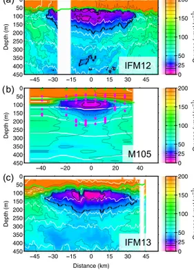
3.1 Vertical eddy structure and its temporal evolution In order to compare the vertical structure of the eddy from the three surveys, all sections were referenced to “kilome- tre distance from the eddy core” as the spatial coordinate, while the “centre” was selected based on visual inspection for the largest vertical extent of the low oxygen core defined by oxygen concentrations below 40 µmol kg−1. In all three sections the core is found in the centre of the eddy (Fig. 2), extending over the depth range from the mixed layer base (50 to 70 m) down to about 200 m depth. The upper and lower boundary aligns with the curvature of isopycnals. Consider- ing the whole section across the eddy, it can be seen that to- wards the centre of the eddy the isopycnals show an upward bending in an upper layer (typically associated with cyclonic- rotating eddies) and a downward bending below (associated with anticyclonic-rotating eddies) which is characteristic of ACMEs.
During the first survey (IFM12), lowest oxygen concen- trations of about 8 µmol kg−1 were observed in two verti- cally separated cores at about 80 and 120 m depth, while in between the two cores, oxygen concentrations increased to about 15 µmol kg−1. About 6 weeks later, during the M105 ship survey, lowest concentrations of about 5 µmol kg−1 were observed, centred at about 100 m depth and without a clear double minimum anymore, based on six CTD sta- tions. During the last glider survey (IFM13), another three weeks after the ship survey, the minimum concentrations were<3 µmol kg−1and showed in the vertical a single min-
Distance (km)
Depth (m)
−45 −30 −15 0 15 30 45 0
50 100 150 200 250 300 350 400 450
Oxygen (µmol kg−1) 0 25 50 100 150 200
Distance (km)
Depth (m)
−40 −20 0 20 40
0 50 100 150 200 250 300 350 400 450
Oxygen (µmol kg−1) 0 25 50 100 150 200
Distance (km)
Depth (m)
−45 −30 −15 0 15 30 45 0
50 100 150 200 250 300 350 400 450
Oxygen (µmol kg−1) 0 25 50 100 150 200
IFM12
M105 a)
b)
IFM13 c)
(
(
(
Figure 2.Oxygen distribution from the three eddy surveys (see Fig. 1) in reference to distance (0 km is set at a subjectively se- lected eddy centre):(a)glider IFM12,(b)ship M105, and(c)glider IFM13. The 15 µmol kg−1(40 µmol kg−1) oxygen contour is indi- cated as a bold (broken) black line. Selected density anomaly con- tours are shown as white lines (1σ=0.2 kg m−3). The green line indicates the mixed layer base. The oxygen contour in(b)was grid- ded based on the eight CTD stations (locations indicated by the green stars at 0 dbar) and mapped to a linear section in latitude, longitude. In(b) the magenta dots indicate positions of local N2 maxima in the CTD profiles.
imum centred at about 120 m. The intensification of the min- imum (by about 5 µmol kg−1in 2 months) is assumed here to be a result of continued respiration without balancing lat- eral/vertical mixing oxygen supply. It is important to note that during the glider survey the eddy performed about one full rotation and hence we expect less impact of the spatial variability in our sampling of the core. Underneath the eddy core, and best seen in the 40 µmol kg−1oxygen contour be- low 350 m at about 0 km (centre), an increase in oxygen over time is found, indicating supply of oxygen from surrounding waters. Comparing the two glider surveys (Fig. 2), a broaden- ing of the gradient zone at the upper boundary of the core is observed. Overall the upper boundary of the core during the first survey aligned tightly with the mixed layer base, giv- ing the core the shape of a plano-convex lens, while the lens developed into a biconvex shape before the second glider sur- vey (also seen in the ship survey, Fig. 2b).
The SLA data analysis for the eddy (see Schütte et al., 2016b, for details) suggests a formation in the Mauritanian upwelling region (Fig. 1). The composite of the outermost
Distance (km)
Depth (m)
−45 −30 −15 0 15 30 45 0
50 100 150 200 250 300 350 400 450
Absolute salinity (g kg)−1
35.2 35.4 35.6 35.8 36 36.2 36.4 36.6 36.8
Distance (km)
Depth (m)
−45 −30 −15 0 15 30 45 0
50 100 150 200 250 300 350 400
450 °Conserv. temperature ( C)
11 12 13 14 15 16 17 18 19 20 21 22
Distance (km)
Depth (m)
−45 −30 −15 0 15 30 45 0
50 100 150 200 250 300 350 400 450
N2 (10−5 s−2)
0 1 2 3 4 5 6 7 8 9 10 11 12
Distance [km]
Depth [m]
−45 −30 −15 0 15 30 45 0
50 100 150 200 250 300 350 400 450
Turner angle
−90
−45 0 45 90
a) (
b) (
c) (
(d)
Figure 3. (a)SA,(b)2,(c)N2, and(d)Turner angle (only seg- ments|45 to 90|are shown) from the IFM12 survey. The thick black broken line indicates the 40 µmol kg−1oxygen concentration indi- cating the low oxygen core (see Fig. 2). The green line indicates the mixed layer base. Selected density anomaly contours are shown as white lines (1σ=0.2 kg m−3).
(“last”) closed geostrophic contour of the eddy (Fig. 1, right) revealed a diameter of about 60 km, which is in accordance with the dimensions of the vertical structures observed from the glider and the ship (Figs. 2 and 3). The eddy core is com- posed of a fresh and cold (Figs. 3a, b and 4a) water mass that matches the characteristics of South Atlantic Central Water (SACW; Fiedler et al., 2016) and is a typical composition for low oxygen eddies in the eastern tropical North Atlantic (Karstensen et al., 2015; Schütte et al., 2016a, b). The prop- erties confirm that the ACME was formed in the coastal area off Mauritania, as suggested by the SLA analysis (Schütte et al., 2016b; Fig. 1, left). Layering of properties, as seen in oxygen (Fig. 2), is also observed in SA and2 (Fig. 3) un- derneath the eddy core. In the depth range between 160 and 250 m the layers are aligned with density contours and sug- gest isopycnal transport processes, while below that depth range, and at the edges of the eddy core, the thermohaline intrusions cross density surfaces.
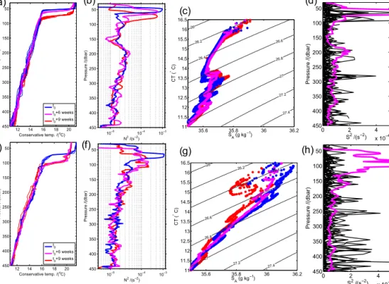
The low oxygen core of the ACME is well separated from the surrounding water through maxima inN2(Fig. 3c). The most stable conditions (N2about 3 to 5×10⁻⁴s−2; compare Fig. 4a) are found along the upper boundary of the core and aligned with the mixed layer base (changed from 50 to 70 m between IFM12 and IFM13, respectively). 2 (SA) differ- ences across the mixed layer base were large, about 5 to 6 K (0.7–1.0 g kg−1), but over time the mixed layer base widened from 8 m (glider IFM12 survey) to 16 m (M105 ship) and to 40 m (glider IFM13 survey) (Fig. 4a).
At the lower side of the ACME theN2maximum was an order of magnitude weaker (N2∼4×10⁻⁵s−2), but sepa- rates the eddy core well from the surrounding waters. The layering in properties is also seen in alternating patterns in N2at the rim and below the eddy. A possible driver for mix- ing in this region is double diffusion, and therefore the sta- bility ratioRρ= αθ2z
βθ(SA)z (McDougall and Barker, 2011) was calculated.Rρ is the ratio of the vertical (z) gradient in2, weighted by the thermal expansion coefficient (α2), over the vertical (z) gradient inSA, weighted by the haline contraction coefficient (β2)(Fig. 3d). For convenienceRρ is converted here to a Turner angle (Tu) using the four-quadrant arctan- gent. ForTubetween−45 and−90◦the stratification is sus- ceptible to salt-finger type double diffusion, whileTu+45 to +90◦indicate susceptibility to diffusive convection. Regions where double diffusion most likely occurs are found forTu close to±90◦.
In the core of the eddy theTuindicates a weak salt-finger regime (Tuvalues close to+45◦; Fig. 3d); however, no well- developed thermohaline gradients exist and thus no enhanced vertical mixing by double diffusion is expected to take place here. In contrast, below the low oxygen core and along the thermohaline layering structures, theTupatterns show values within the±45 to ±90◦ range, even getting close to±90◦. At both edges (±15 to±45 km) a band of diffusive convec- tion is seen and here is where water of the core potentially exchanges/erodes (see below). TheTupattern does not align with the tilting of the isopycnals, but crosses isopycnals. The thermohaline gradients are most likely created by intrusions of cold and saline SACW from the core into the surrounding warm and salty water. The core itself shows a2/SA char- acteristic of constant slope over time (Fig. 4c) and indicat- ing weak mixing with surrounding water. The salinity offset between gliders IFM12 and IFM13 is about−0.01 g kg−1, which could indicate a weak exchange of the whole core (all densities) with surrounding water, but also is close to the expected accuracy of the salinity data. What clearly is evi- dent is a shrinking of the core2/SArange from 15.7/13.7 to 15.2/13.9◦C.
At the edge region of the eddy (Fig. 4e to g) the mixed layer base is wider and the gradient is less sharp (Fig. 4e) when compared with the centre of the eddy (Fig. 4a). No low N2core and thus no doubleN2maxima are found, but just one maximum (much weakerN2∼10−4s−2)at the mixed
35.6 35.8 36 36.2 11
11.5 12 12.5 13 13.5 14 14.5 15 15.5 16
16.5 26
26.2 26.4
26.6
26.8
27
27.2 27.4
S (g kg )A −1 CT (° C)
10−5 10−4 10−3
50 100 150 200 250 300 350 400
450
N2 /(s−2)
Pressure /(dbar)
12 14 16 18 20
50
100
150
200
250
300
350
400
450
Conservative temp. /( C)o
Pressure /(dbar)
t0 t0+6 weeks t0+9 weeks
0 2 4
x 10−4 50
100 150 200 250 300 350 400 450
Pressure /(dbar)
S2 /(s−2)
0 2 4
x 10−4 50
100 150 200 250 300 350 400 450
Pressure /(dbar)
S2 /(s−2)
10−5 10−4 10−3
50
100 150 200 250 300
350 400
450
N2 /(s−2)
Pressure /(dbar)
12 14 16 18 20
50
100
150
200
250
300
350
400
450
Conservative temp. /( C)o
Pressure /(dbar)
t0 t0+6 weeks t0+9 weeks
( a) ( b) ( d)
35.6 35.8 36 36.2
11 11.5 12 12.5 13 13.5 14 14.5 15 15.5 16 16.5 26
26.2
26.4
26.6
26.8
27
27.2
27.4
S (g kg ) A
−1 CT (° C)
( c)
( e) ( f)
( g) ( h)
Figure 4.Eddy centre profiles for(a)2and(b)buoyancy frequencyN2, the(c)2/SAdiagram, and(d)vertical shear of horizontal velocities (S) squared.(e–h)as(a–d)but for selected profiles at the edge of the eddy. In(d, h)the magenta line indicates the magnitude ofS2required to overcome the local stability (4·N2).
layer base (Fig. 4f) is found, at least for the ship (M105) and the second glider survey (IFM13). Overall theN2 maxima are located deeper in the water column. The2/SAdiagram (Fig. 4g) shows more of the characteristics of the surrounding waters but thermohaline intrusions for temperatures below 13.8◦C which have a water mass core moving along isopyc- nals.
The ADCP zonal velocity data from the M105 ship survey show a baroclinic, anticyclonic-rotating flow, with a maxi- mum swirl velocity of about 0.4 m s−1 at about 70 m depth and 30 km distance from the eddy centre (Fig. 5a). The max- imum rotation speed (see as an approximation the zonal ve- locity, Sect. 5a) decreases nearly linearly to about 0.1 m s−1 at 380 m depth. Considering the translation speed of the eddy of 3 to 5 km day−1 (Schütte et al., 2016b), the nonlinearity parameterα, relating maximum swirl velocity to the trans- lation speed, is much larger than 1 (about 6.5 to 11 in the depth level of the low oxygen core) and indicates a high co- herence of the eddy (Chelton et al., 2011). At the depth of the maximum swirl velocity, and considering the eddy radius of 30 km, a full rotation would take about 5 days, but even longer for the deeper levels.
To investigate the flow field we decompose the observed velocity (u, v) into a mean (u,¯ v)¯ and a fluctuating part (u0, v0) by applying a 120 m boxcar filter (a longer filter length does not significantly change the results) to the ob-
served profile data (here for the zonal velocityu, Fig. 5a, b, c):
u= ¯u+u0.
Thev¯ field is here interpreted as the mesoscale or “subin- tertial” flow (Fig. 5b) and shows a baroclinic anticyclonic circulation with velocity maximum close to the surface at
±30 km in the eddy-relative coordinates. The fluctuating part (u0; Fig. 5c) is dominated by alternating currents with about 80 to 100 m wavelength. This layering of velocity finestruc- ture resembles layering in properties (Figs. 2 and 3) and in- dicates shears most likely introduced by the propagation of NIWs (Joyce et al., 2013; Halle and Pinkel, 2003). Largestu0 currents are found in two regions: (i) in the upper 150 m in the vicinity of the mesoscale velocity maximum at the south- western side of the eddy (Reg. 1) and (ii) in the 250 to 450 m depth range below the core (Reg. 2). We estimated the pro- gressive vector diagram (PVD) of theu0 fluctuating veloc- ity components for the two regions and found cyclonic rota- tion, indicating the downward vertical energy propagation of NIWs (Leaman and Sanford, 1975). However, for the region at the eddy edge (Reg. 1) the levels below 150 m depth show no rotation in the PVD, suggesting that the downward energy propagation does not continue, which may suggest either re- flecting or dissipation (e.g. Kunze et al., 1995).
From the subinertial velocity field the relative vorticity was calculated and subsequently the feff across the eddy
−0.2 0 0.2 0.4 0.6
−0.05 0 0.05 0.1 0.15 0.2
cumsum(u’) ms−1
cumsum(v’) ms−1
−0.6 −0.4 −0.2 0 0.2
−0.4
−0.2 0 0.2 0.4
cumsum(u’) ms−1
cumsum(v’) ms−1
Distance (km)
Depth (m)
−45 −30 −15 0 15 30 45 0
50 100 150 200 250 300 350 400 450
u (m s−1)
−0.4
−0.2 0 0.2 0.4
u (m s-1)
(a)
(e)
Region 1 Region 2
Distance (km)
Depth (m)
−45 −30 −15 0 15 30 45 0
50 100 150 200 250 300 350 400
450 −0.4
−0.2 0 0.2 0.4
u (m s-1)
(b)
Distance (km)
Depth (m)
−45 −30 −15 0 15 30 45 0
50 100 150 200 250 300 350 400 450
u’ (m s−1)
−0.1
−0.05 0 0.05 0.1
1
u’ (m s-1)
2
(c)
Distance (km)
Depth (m)
−45 −30 −15 0 15 30 45 0
50 100 150 200 250 300 350 400 450
eff
0.6 0.7 0.8 0.9 1 1.1 1.2 1.3 1.4
feff / f
1
2
(d)
Figure 5. (a)Observed zonal velocity,(b)boxcar filtered zonal velocity (applied over 120 m), and the(c)difference between observed and boxcar filtered velocities. The thick black broken line indicates the 40 µmol kg−1oxygen concentration; white contours are selected density anomaly contours (1σ=0.2 kg m−3)determined by gridding CTD profile data (see the green stars at 0 dbar for station positions). The yellow dots indicate theN2maximum from CTD profile data.(d)Ratio between the effective Coriolis parameter (feff)and local Coriolis parameter(f).(e)Progressive vector diagram ofu0/v0for regions 1 (250 to 450 m depth, seven profiles) and 2 (20 to 140 m; three profiles) (seecanddfor locations); the black dots mark the shallowest depth
(Fig. 5d). Within the core of the anticyclone (ζ <0)afeff<
f withRo= −0.7 between 70 and 150 m is found. At the transition between eddy and surrounding waters ζ changes sign and a positive vorticity ridge (feff/f >1.3) is observed.
Likewise, a local increase in feff is seen underneath the core in the eddy centre. In both regions large amplitude u0 (Fig. 5c) andv0 (not shown) are observed as well as down- ward NIW energy propagation (from PVD; Fig. 5e).
An aliasing occurs through the rotation of the inertial cur- rent vector during the survey time. Joyce et al. (2013), in their analysis of mid-latitude NIW propagation (inertial pe- riod 19 h), applied a back rotation. However, at 19◦N the in- ertial period is 36.7 h and the complete ADCP section was surveyed within 14 h (including station time). Because we primarily interpret station data, the aliasing effect should be small for the M105 data. In contrast, the glider sections took several days and many inertial periods, and thus a mixture of time–space variability is mapped in the property fields (Figs. 3 and 4). It is however interesting to note that the ve- locity and property layering still looks very similar and co- herent across the different surveys, suggesting that the pro- cesses that drive the layering are rather long-lasting over sev- eral months.
3.2 Eddy core isolation and vertical fluxes
Karstensen et al. (2015) proposed a concept for the forma- tion of a low oxygen core in a shallow ACME in the eastern tropical North Atlantic as a combination of isolating the eddy core against oxygen fluxes (primarily vertical) and high pro- ductivity and subsequent respiration of sinking organic ma- terial. The concept is in analogy to the formation of dead zones in coastal and limnic systems, hence the name “dead zone eddies”. The key for high productivity is the transport of nutrients into the euphotic zone in the eddy.
We identified three areas in the eddy where we further analysed vertical transport and mixing: (Area I) the eddy core, bounded by N2 maxima with a low stratification in between. (Area II) The layering regime underneath the low oxygen core with alternating velocity shear and density com- pensated, mainly salt-finger supporting thermohaline intru- sions. (Area III) The high velocity shear zones at the south- eastern edge of the eddy and underneath the eddy centre. We do not have direct mixing estimates (e.g. microstructure) but analyse the observedS2,N2, andRifrom the M105 ship sur- vey data. Selected CTDN2profiles from the centre and the edge of the eddy are analysed in combination with ADCP fluctuation velocity (u0, v0) shear, estimated from 8 m bin data (Fig. 4d, h). To take the high-frequency temporal fluc-
tuations in the velocity data into account we show here the velocity shear in the vicinity of the CTD station, consider- ing all ADCP data recorded 30 min before until 60 min after the CTD station started. Based on the existing (1 dbar) N2 we calculated aS2that satisfied aRi<1/4 (magenta line in Fig. 4d, h).
For the eddy core (Area I) a strong contrast to surrounding water masses is seen across the mixed layer base, but also laterally (Fig. 4c). Decreasing oxygen concentrations are ob- served in Area I over a period of 2 months, while the2/SA characteristics exhibit a stable slope (Fig. 4). Low mixing in the core of ACMEs has been explained from direct observa- tions before. Sheen et al. (2015) and Kawaguchi et al. (2016) observed enhanced mixing at the N2 maximum and found wave–wave interaction as a likely process for the mixing.
They argued that, because of the N2 maximum around the core, but also because of the lowN2in the core, less wave energy can enter the core and mixing in the core is low. Halle and Pinkel (2003) argued that, because of the lowN2in the core, the NIW energy density was low and hence less en- ergy is available for mixing. Our observations do show that high mixing occurs at the N2maxima and that the core it- self is a low mixing regime. The mixing to take place at the N2 maximum is seen in a widening and deepening of the gradient zone at the mixed layer base in all sections and is even stronger towards the edges of the eddy (Figs. 2, 3, and 4a). The consequence of vertical change from a high to a low mixing zone creates an “erosion” (outward directed mixing) of the core into the mixed layer. The erosion is linked to up- welling and thus it has implications for the oxygen and nu- trient cycling, as will be discussed below.
In the layering shear regime underneath the eddy (Area II) we found that Ri approaches critical values (1/4) in layers of maximal NIW velocity-induced shear and thus may in- dicate generation of instabilities in these layers. Below the eddy theSAgradients (Fig. 3a) do align with the wave crests, indicating the impact of intense strain, and thus a periodic in- tensification ofSAgradients, which in turn could enhance the susceptibility to double diffusive mixing (Fig. 3d). Likewise the2/SAdiagram clearly shows the existence of thermoha- line intrusions oriented along isopycnals.
Area III is where high u0 shear is observed (Reg. 1 and Reg. 2; Fig. 5c, d). It is plausible to assume that a large frac- tion of the NIW energy that impacts the eddy originates from wind stress fluctuations (D’Asaro, 1985). The NIW energy propagation in the upper layer of the eddy (above the core) is downward, across the intenseN2contours/mixed layer base, and possibly driving enhanced mixing (e.g. by wave–wave interaction as in Sheen et al., 2015). TheRi(Fig. 4d, h) in- dicates that at the mixed layer base where high shear and highN2are found. In the eddy coreN2is low, but so is the shear (Fig. 4d). At the eddy edge (∼ −32 km distance), in the transition between maximum swirl velocity and the sur- rounding ocean, NIW energy is forced to propagate down- ward (see Fig. 4b, d) because feff/f >1 (Fig. 5b). The Ri
distribution (Fig. 4h) for the M105 ship survey shows thatN2 is too high to be destabilized by the shear, at least at the lo- cation where the CTD profile was taken. However, we know that the NIWs have an amplitude of more than 0.1 m s−1and a vertical scale of about 70 to 90 m (Fig. 4d). This is sim- ilar to observations at mid-latitude fronts (e.g. Whitt et al., 2014; Kunze and Sanford, 1984) where an inertial radius of about 2 km for an amplitude of 0.1 m s−1has been found and thus such a wave covers a good part of the eddy front. More- over, the magnitude of the fluctuation (0.1 m s−1)associated with the NIW accounts for about 25 % of maximum swirl velocity at about∼ −32 km at 50 to 120 m depth. The NIW phase velocity(u0; Fig. 5c) is of a similar magnitude to the swirl velocity and thus susceptible to critical layer formation (Kawaguchi et al., 2016). For a Gulf Stream warm core ring, Joyce et al. (2013) found most instabilities and mixing close to the surface and where most horizontal shear in the baro- clinic current is found (similar to our region 1; Fig. 5c, d).
Evidence for vertical mixing to take place in this region is seen in upwelling of nitrate into the mixed layer/euphotic zone at about 100 m depth/distance of about −32 km (see below; Fig. 7b). Underneath the eddy the vertical propaga- tion of superinertial waves across the anticyclonic eddy is seen (Kunze et al., 1995) but into a region wherefeff/f >1 (Reg. 2 in Fig. 5c, d) and whereRiis getting critical, possibly related to a slowing of the energy propagation.
3.3 Nutrient cycling in the eddy
The productivity associated with the ACME requires the up- ward fluxes of nutrients into the euphotic zone. Schütte et al. (2016b) showed that the low oxygen ACMEs in the trop- ical eastern North Atlantic do have productivity maxima (in- dicated by enhanced ocean colour based chlorophyll a es- timates) to be more concentrated at the rim of the eddies.
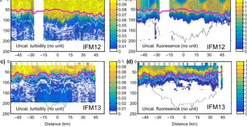
This observation suggests that the vertical flux is also con- centrated at the rim of the eddy. Indeed, when inspecting the glider section data (Fig. 3) we do find evidence for upwelling being concentrated at the rim, although the mixed layer base is characterized by very stable stratification and large gra- dients (e.g. 0.3 K m−1in temperature). Considering the first glider oxygen section (IFM12, Fig. 2a), the upper of the two separate oxygen minima is found very close to the depth of the mixed layer base and indicates that any exchange across the mixed layer by mixing processes must be very small. The number of particles might be approximated by the turbidity measurement from the glider (Fig. 6a, c). While the first sur- vey had very high turbidity several tens of metres below the mixed layer base (Fig. 6a), the second glider survey showed much less particle load (Fig. 6c), indicating lower produc- tivity across the eddy that may be related to a weakening of the vertical flux of nutrients into the euphotic zone. The flu- orescence signal (Fig. 6b, d) indicates the first glider survey (IFM12, Fig. 6b) captured a bloom that occupied the whole mixed layer (note that the periods with low fluorescence align
Distance (km)
−45 −30 −15 0 15 30 45 0
50 100 150 200
250 00.10.20.30.40.50.60.70.80.911.11.21.3
Distance (km)
Depth (m)
−45 −30 −15 0 15 30 45 0
50 100 150 200 250
uncal. Chl−a [νgr l−1]
00.1 0.20.3 0.40.5 0.60.7 0.80.9 11.1 1.2 1.3 Distance (km)
Depth (m)
−45 −30 −15 0 15 30 45 0
50 100 150 200
250 0
0.01 0.02 0.03 0.04 0.05 0.06 0.07 0.08 0.09 0.1
U ncal. turbidity (no unit) ( a)
Distance (km)
Depth (m)
−45 −30 −15 0 15 30 45 0
50 100 150 200 250
uncal. Turbidity [no unit]
0 0.01 0.02 0.03 0.04 0.05 0.06 0.07 0.08 0.09 0.1
U ncal. turbidity (no unit)
b)
IFM12
IFM13
U ncal. fluoresence (no unit) IFM12
IFM13
U ncal. fluoresence (no unit) d)
c)
( ((
Figure 6.Uncalibrated turbidity(a, c)and chlorophyll-fluorescence(b, d)data from the glider IFM12 survey(a, b) and glider IFM13 survey(c, d). The magenta line denotes the base of the mixed layer; the broken black line is the extent of the low oxygen core (oxygen
<40 µmol kg−1).
with daylight periods and as such are generated by quench- ing) and as such intense nutrient supply and productivity. In contrast, the second glider survey (IFM13; Fig. 6d) shows a clear subsurface fluorescence maximum (about 10 m above the mixed layer base), indicating that the nutrient supply is primarily concentrated on mixed layer base exchange pro- cesses.
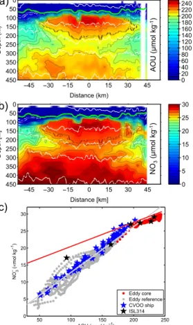
In order to interpret the low oxygen concentrations in terms of biogeochemical processes, the bulk remineraliza- tion of oxygen and nitrate is determined. The apparent oxy- gen utilization (AOU, Fig. 7a) is defined as the difference be- tween measured oxygen concentration and the oxygen con- centration of a water parcel of the given2andSAthat is in equilibrium with air (Garcia and Gordon, 1992, 1993). AOU is an approximation for the total oxygen removal since a wa- ter parcel left the surface ocean. The low oxygen concen- trations in the core of the eddy are equivalent to an AOU of about 240 µmol kg−1 (Fig. 7a). Along with high AOU we also find very high NO−3 concentrations with a maxi- mum of about 30 µmol kg−1 (Fig. 7b). The corresponding AOU : NO−3 ratio outside the core is 8.1 and thus close to the classical 8.625 Redfield ratio (138/16; Redfield et al., 1963).
However, in the core an AOU : NO−3 ratio of>16 is found.
This high ratio indicates that less NO−3 is released dur- ing respiration (AOU increase) than expected for a reminer- alization process following a Redfieldian stoichiometry. By considering the remineralization outside the core (Fig. 7c) the respective NO−3 deficit can be estimated to up to 4–
6 µmol kg−1 for the highest AOU (NO−3)observations. By integrating NO−3 and NO−3 deficit over the core of the low oxygen eddy (defined here as the volume occupied by water with oxygen concentrations <40 µmol kg−1) we obtain an average AOU : NO−3 ratio of about 20 : 1.
One way to interpret this deficit is by NO−3 loss through denitrification processes. Löscher et al. (2015) and Grundle et al. (2017) both found evidence for the onset of denitri- fication in the core of the ACME discussed here. Oxygen concentrations in the core are very low (about 3 µmol kg−1) and denitrification is possible. Evidence for denitrification in the core of the ACME was, however, demonstrated as being important for nitrous oxide (N2O) cycling at the nanomolar range (Grundle et al., 2017), and not necessarily for overall NO−3 losses, which are measured in the micromolar range.
Grundle et al. (2017) showed by relating nitrogen and phos- phorous cycling that in the core of the ACME the NO−3 losses were not detectable at the micromolar range. Thus, while denitrification may have played a minor role in causing the higher than expected AOU : NO−3 ratio which we have cal- culated, it is unlikely that it contributed largely to the loss of 5 % of all NO−3 from the eddy as estimated based on the observed AOU : NO−3 ratios.
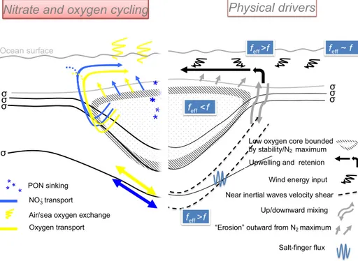
Alternatively, but perhaps not exclusively, the NO−3 recy- cling within the ACME could be the reason for the NO−3 deficit. A high AOU : NO−3 ratio could be explained through a decoupling of NO−3 and oxygen recycling pathways in the eddy and details about the vertical transport pathways of nu- trients (erosion of the core). Based on the investigation of the possible vertical mixing/transport of nutrients (here NO−3) the erosion of the eddy core plays a key role. In this sce- nario NO−3 molecules are used more than one time for the remineralization/respiration process, and therefore the AOU increases without a balanced, in a Redfieldian sense, NO−3 remineralization. Such a decoupling can be conceptualized as follows (Fig. 8, left): consider an upward flux of dissolved NO−3 and oxygen in a given ratio with an amount of water that originates from the low oxygen core. The upward flux partitions when reaching the mixed layer; one part disperses