D I S S E R T A T I O N
zur Erlangung des akademischen Grades Doctor Rerum Naturalium
(Dr. rer. nat.) im Fach Physik eingereicht an der
Mathematisch-Naturwissenschaftlichen Fakultät I
Humboldt-Universität zu Berlin von
Sami Kama
geboren am 18.09.1978 in Biga/Türkiye Präsident der Humboldt-Universität zu Berlin:
Prof. Dr. Dr. h.c. Christoph Markschies
Dekan der Mathematisch-Naturwissenschaftlichen Fakultät I:
Prof. Dr. Lutz-Helmut Schön Gutachter:
1. Prof. Dr. Hermann Kolanoski 2. Dr. Klaus Mönig
3. Prof. Dr. Torbjörn Sjöstrand
improve our current knowledge of the physics these events must be understood.
However, the physics of soft interactions are not completely known at such high en- ergies. Different phenomenological models, trying to explain these interactions, are implemented in several Monte-Carlo (MC) programs such as PYTHIA, PHOJET and EPOS. Some parameters in such MC programs can be tuned to improve the agreement with the data.
In this thesis a new method for tuning the MC programs, based on Genetic Al- gorithms and distributed analysis techniques have been presented. This method represents the first and fully automated MC tuning technique that is based on true MC distributions. It is an alternative to parametrization-based automatic tuning.
This new method is used in finding new tunes for PYTHIA 6 and 8. These tunes are compared to the tunes found by alternative methods, such as the PROFESSOR framework and manual tuning, and found to be equivalent or better. Charged parti- cle multiplicity,dNch/dη, Lorentz-invariant yield, transverse momentum and mean transverse momentum distributions at various center-of-mass energies are generated using default tunes of EPOS, PHOJET and the Genetic Algorithm tunes of PYTHIA 6 and 8. These distributions are compared to measurements from UA5, CDF, CMS and ATLAS in order to investigate the best model available. Their predictions for the ATLAS detector at LHC energies have been investigated both with generator level and full detector simulation studies.
Comparison with the data did not favor any model implemented in the generators, but EPOS is found to describe investigated distributions better. New data from ATLAS and CMS show higher than expected multiplicities and a faster rise with the center-of-mass energy in central particle multiplicity.
Wechselwirkungen, deren überlagerte Signale vom Detektor gemessen werden. Diese Ereignisse müssen so präzise wie möglich verstanden werden, um einerseits neuartige physikalische Phänomene zu entdecken, andererseits aber dazu beitragen, das Ver- ständnis bereits bestehender physikalischer Gesetze zu verbessern. Inbesondere ist die Physik der weichen Wechselwirkungen momentan noch nicht genau verstanden.
Unterschiedliche theoretische Modelle, die versuchen, diese Physik zu beschreiben, sind in Monte-Carlo (MC) Generatoren wie EPOS, PHOJET und PYTHIA einge- bunden. Deren Modelle sind auf mannigfaltige Weise parametrisierbar und müssen mit experimentellen Daten angepasst werden.
In dieser Arbeit wird eine neue Methode, basierend auf genetischen Algorithmen und verteilten Analysetechniken, vorgestellt, um diese MC-Parameter anzupassen.
Diese Methode stellt einen alternativen Ansatz zu derzeit verfügbaren Methode wie PROFESSOR dar mit dem Vorteil, dass die Suche nach geeigneten Modellparame- tern automatisiert ist.
Der Ansatz der genetischen Algorithmen wurde benutzt, um für PYTHIA 6 und PYTHIA 8 Parameter zu finden, die gut mit bisherigen Messungen übereinstimmen.
Die Ergebnisse wurden mit den MC-Generatoren EPOS und PHOJET und Daten von UA5 CDF, CMS und ATLAS verglichen, wobei eine Reihe von charakteristi- schen Verteilungen untersucht wurden wie Multiplizitäts- Spektren geladener Teil- chen sowie Lozentz-invariante Größen. Auch Vorhersagen für LHC-Energien werden sowohl auf Generator level als auch nach kompletter ATLAS-Detektor-Simulation präsentiert.
Datenvergleiche beveoruzugen nicht eindeutig eines der in die Generatoren imple- mentierten Modelle, jedoch beschreibt EPOS die untersuchten Verteilungen etwas besser. Neue Daten von ATLAS und CMS zeigen höhere Multiplizitäten als erwartet und einen schnelleren Anstieg der zentralen Multiplizität mit der Schwerpunktsener- gie.
2. LHC and ATLAS 3
2.1. The Large Hadron Collider . . . 3
2.2. ATLAS Detector . . . 5
2.2.1. Inner Detector . . . 6
2.2.2. Calorimetry . . . 11
2.2.3. Muon Systems . . . 20
3. Trigger and Data Acquisition in ATLAS 25 3.1. Level-1 Trigger . . . 25
3.1.1. Level-1 Muon Trigger . . . 29
3.1.2. Central Trigger Processor . . . 30
3.2. Data Acquisition and High-Level Trigger . . . 31
3.3. Monitoring of ATLAS Trigger and DAQ . . . 36
4. Monte-Carlo Programs 43 4.1. The Standard Model . . . 43
4.2. Event Signatures . . . 47
4.3. Reggeons and Pomerons . . . 49
4.4. Monte-Carlo Event generators . . . 50
4.5. PYTHIA . . . 52
4.6. PHOJET . . . 55
4.7. EPOS . . . 56
5. Monte-Carlo Tuning with Genetic Algorithms 59 5.1. Data . . . 61
5.1.1. CDF . . . 61
5.1.2. DØ . . . 66
5.1.3. UA5 . . . 68
5.1.4. Implementation of analyses . . . 69
5.2. Genetic Algorithms . . . 70
5.3. Application of GA’s to MC Tuning . . . 72
5.4. Tuning PYTHIA 6 and PYTHIA 8 . . . 75
5.5. Results . . . 84
6. Data-MC Comparisons 91 6.1. Multiplicities . . . 91
6.2. Transverse Momentum . . . 96
7. Predictions for LHC energies 107 7.1. Multiplicity distributions . . . 107
7.2. Transverse Momentum Distributions . . . 110
7.3. Average Transverse Momentum . . . 110
7.4. Full Detector Simulation . . . 114
8. Conclusions 125 Appendix 127 A. Operational Monitoring Display 129 A.1. OMD Core . . . 129
A.1.1. IS Gatherer . . . 129
A.1.2. Storage . . . 129
A.1.3. Classifier . . . 129
A.1.4. Histogram Producer . . . 131
A.1.5. Configurator . . . 132
A.2. OMD GUI . . . 132
A.2.1. Subscription Editor . . . 134
A.2.2. Plots and Tables . . . 136
A.2.3. Histogram Configuration . . . 138
A.2.4. Alerts . . . 138
B. Monte-Carlo Comparison Plots 143
C. PYTHIA Tune Comparisons 149
and LHCb. ATLAS and CMS are general purpose detectors, on the other hand LHCb is oriented towards b-quark studies and ALICE is designed for heavy-ion collisions. The LHC, at its nominal design energy of 14 TeV and luminosity L= 1034cm−2s−1, is ex- pected to have 720-920 million interactions per second. Most of these interactions will be soft QCD interactions also known as Minimum Bias (MB) events. The physics of the minimum bias events is not completely understood, yet they are the key for under- standing the detectors and search for new physics. It is estimated that at each bunch crossing at nominal energy and luminosity about 20 minimum bias interactions will take place [1, 2].
Most of the events have to be filtered out since it is impossible to store that much data and only a very small fraction of these events have interesting signatures for new physics. Thus one needs to understand the minimum bias events for searching interesting event signatures and selecting the data to be stored for offline processing. Moreover MB events will affect any measurement significantly. Figure 1.1 shows a simulation of a typical Z →j+j event at the ATLAS detector with and without MB pileup.
The traditional solution for these problems is using Monte-Carlo (MC) programs for estimating the trigger settings and event selection criteria (cuts) for the background subtraction. However since the soft QCD interactions are not yet completely understood, there are different MC programs with different models. The models in such programs usually agree up to some extent with the minimum bias data however their extrapolations to the higher energies are usually quite different. Also these models usually have free parameters that needs to be tuned in order to be able to describe existing data better.
Tuning of the MC programs has been a tedious and subjective task. In this thesis a new method using genetic algorithms and distributed processing is presented for automatic MC tuning.
In chapter 2, a brief introduction to the LHC and the ATLAS experiment is presented.
The data acquisition and trigger systems are discussed and a brief explanation of trigger monitoring is given in chapter 3. Chapter 4 contains a brief introduction to the Standard Model, Monte-Carlo programs and their models. In chapter 5, the Genetic Algorithms and the tuning method is discussed. The data sets used in tuning are also discussed
Figure 1.1.: Simulation of a typical Z0 → j+j event in the ATLAS detector. Top picture shows only the tracks from the event and the bottom picture shows the tracks from the same event together with the tracks from 23 minimum bias events that are expected to happen in the same bunch crossing at the LHC.
(CERN) near Geneva. Construction of the LHC machine was approved by the CERN council in December 1996. In 2000, the Large Electron Positron (LEP) collider was closed and construction of the LHC began. The LHC started operation in September 2008 but a faulty connection caused an accident and it was shutdown until Nowember 2009 for repairs.
At the LHC there are two high luminosity experiments, ATLAS [4] and CMS [5], and two low luminosity experiments LHCb [6] and TOTEM [7]. There is also one dedicated heavy-ion experiment, ALICE [8]. Their locations on the LHC ring and accelerator complex at CERN can be seen in figure 2.1. LHCb is oriented towardsbquark physics, with a peak luminosity of L= 1032cm−2s−1. TOTEM, on the other hand, looks for elastic scattering at small angles, with a peak luminosity ofL= 2·1029cm−2s−1. ALICE aims to study heavy-ion (lead-lead) collisions at a peak luminosity ofL= 1027cm−2s−1. ATLAS and CMS are both general purpose experiments designed to search for physics of the Standard Model and beyond. Only the ATLAS experiment is described here.
Detailed descriptions of the other experiments and their physics goals are available in the respective references.
2.1. The Large Hadron Collider
The Large Hadron Collider (LHC) is a two-ring superconducting hadron accelerator and collider built in the existing 26.7 km tunnel constructed for LEP. The plane of the tunnel lies between 45 m and 170 m below the surface and is inclined at a 1.4% slope towards Lac Léman. Since the tunnel from LEP has been reused, the LHC machine is constrained by the size of the tunnel. Because of this constraint, the machine uses a “two-in-one” super- conducting magnet design. Proton beams in the machine rotate in separate pipes with separate magnetic fields and vacuum chambers except in the insertion and experimental detector regions.
The nominal design center-of-mass energy and peak luminosity of the LHC are 14 TeV andL= 1034cm−2s−1, respectively. To reach 14 TeV, the dipole magnets must generate a nominal magnetic field of 8.33 T. Design luminosity is achieved by injecting 2808
Figure 2.1.: Accelerator complex at CERN. Both proton bunches are accelerated to 450 GeV in several accelerator stages before being injected into the LHC, where they are accelerated up to 7 TeV. The locations of the four major experiments at the LHC ring are also shown.
At peak operation, with a total beam current of 0.584 A, the LHC will have about 1 GJ of energy stored in the beams and magnets. In case of emergency, the beams will be dumped into a graphite target and the magnet systems will be forcibly quenched by quench heaters. Magnetic energy is dispersed with heaters and dump resistors.
2.2. ATLAS Detector
The ATLAS experiment is one of the two general purpose experiments at the LHC. AT- LAS is an acronym forA ToroidalLHCApparatuS. The ATLAS Collaboration aims to measure the Standard Model parameters and search for new physics phenomena. Pre- cise tracking and calorimetry information are needed to accomplish these physics goals requiring a state-of-the-art detector. The ATLAS detector has been built to meet these requirements with the performance goals listed in table 2.1. It has a cylindrical shape and is composed of several layers of sub-detectors. As shown in figure 2.2, the layout of the detector from inside to outside is: Pixel Detector, Silicon Microstrip Detector, Tran- sition Radiation Tracker, Solenoid Magnet, Liquid Argon Electromagnetic Calorimeters and Tile Calorimeters, Toroidal Magnets, Monitored Drift Tubes, Resistive Plate Cham- bers and Thin Gap Chambers. The first three form the Inner Detector, the second three form the calorimetry systems and the last three form the muon systems.
Detector Required η coverage
Component resolution Measurement Trigger Tracking σpT/pT = 0.05%·pT⊕1% ±2.5
EM Calorimetry σE/E = 10%/√
E⊕0.7% ±3.2 ±2.5
Hadronic
Calorimetry(jets)
barrel and endcap σE/E= 50%/√
E⊕3% ±3.2 ±3.2
forward σE/E = 100%/√
E⊕10% 3.1<|η|<4.9 3.1<|η|<4.9
Muon σpT/pT = 10%
±2.7 ±2.4
spectrometer atpT= 1 TeV
Table 2.1.: ATLAS detector performance goals. The symbol ⊕ represents addition in quadrature.
ATLAS uses the nominal interaction point to define a right-handed coordinate system.
Thez-direction of the coordinate system lies on the LHC beam line such that the positive
the opening angle from the +z-axis. The pseudo-rapidity,η, is defined asη=−ln tanθ/2 and distance in theη–φplane is defined as ∆R = p∆η2+ ∆φ2.
In the following sections of this chapter, the parts of the ATLAS detector are briefly described. Details of the detector can be found in [1, 2, 4] and the references therein.
2.2.1. Inner Detector
The Inner Detector produces high precision measurements of charged particle tracks. In order to achieve the physics goals of the experiment it is designed to provide excellent momentum resolution for both primary and secondary vertex measurements of charged particles down topT = 100 MeV within the pseudo-rapidity range |η|<2.5. Figure 2.3 shows one-quarter of the sub-detectors and their distances from the nominal interaction point. The Inner Detector resides in a 2 T solenoidal magnetic field and has a cylindrical shape with boundaries±3512 mm in length and 1150 mm in radius. It is the innermost part of the detector, surrounding the beam pipe and therefore is the most irradiated component of the detector. The design of the Inner Detector is constrained by the requirement of high precision, limits of existing technology, extreme running conditions and by the costs. In order to meet the requirements, it has been designed in three independent but complementary parts. The innermost part, the Pixel Detector, provides high resolution space points. The middle part, the SemiConductor Tracker (SCT) is a silicon strip detector which complements the pixel space points with stereo pairs of silicon microstrip layers. The outermost Inner Detector layer, the Transition Radiation Tracker (TRT), provides continuous tracking to enhance pattern recognition, thereby improving the momentum resolution, as well as electron and pion identification complementary to that of the calorimeters. Figure 2.4 shows the cut-out view of the Inner Detector.
Due to the extreme conditions near the interaction point, the innermost layer of the Pixel Detector will need to be replaced after three years of operation at design luminosity.
In order to keep the noise levels manageable, the silicon sensors are kept at temperatures between−5◦C to−10◦C which corresponds to coolant temperatures of∼ −25◦C. How- ever the TRT operates at room temperatures. Thus the mechanical structure has been designed to able to withstand such temperature gradients with minimal distortions.
Pixel Detector
The Pixel Detector is composed of 1744 pixel sensors. The sensor modules are placed on three cylindrical layers, layer 0, 1 and 2, in the barrel region and on three disks in the endcap regions on both sides. The barrel layers extend from z = −400.5 mm to z= 400.5 mm and reside at radial distances ofR = 50.5, 88.5 and 122.5 mm. The disks are located at z = ±495, ±580 and ±650 mm covering the radial range 88.5 < R <
149.6 mm. This setup of the layers and disks provides spacepoints for charged particles within|η|<2.5.
Each sensor module has a size of 19 x63 mm2. They will initially be operated at
∼ 150 V bias voltage which can be increased up to 600 V throughout the lifetime of the experiment. 90% of the chips have pixels with dimensions of 50x400µm2 and the
Figure 2.2.: The ATLAS detector with its sub-detectors. It has a diameter of 25 m, a width of 44 m and weighs 7000 tonnes.
Envelopes Pixel SCT barrel SCT end-cap
TRT barrel TRT end-cap
255<R<549mm
|Z|<805mm
251<R<610mm 810<|Z|<2797mm
554<R<1082mm
|Z|<780mm
617<R<1106mm 827<|Z|<2744mm
45.5<R<242mm
|Z|<3092mm
Cryostat PPF1
Cryostat Solenoid coil
z(mm)
Beam-pipe Pixel
support tube
SCT (end-cap) TRT(end-cap)
1 2 3 4 5 6 7 8 9101112 1 2 3 4 5 6 7 8
Pixel
400.5 495
580 650
749 853.8
934 1091.5
1299.9 1399.7
1771.4 2115.2 2505 2720.2 0
0 R50.5 R88.5 R122.5 R299 R371 R443 R514 R563 R1066 R1150
R229 R560
R438.8 R408 R337.6 R275
R644 R1004 848 2710
712 PPB1
Radius(mm)
TRT(barrel)
SCT(barrel)
Pixel PP1 ID end-plate 3512
Pixel
400.5 495 580 650 0
0 R50.5 R88.5 R122.5
R88.8 R149.6
R34.3
Figure 2.3.: One quarter of the sub-detectors of the Inner Detector with their distances from the nominal interaction point in mm. The top picture shows the barrel and endcap regions of the TRT, SCT and Pixel Detector. The bottom picture shows a close-up of the Pixel Detector layout.
Figure 2.4.: A 3D rendered image of the Inner Detector. The Pixel Detector, in the center, is surrounded by the SCT barrel layers. TRT straws are placed after SCT layers. Pixel and SCT endcap disks are visible on both sides. Note that SCT endcap disks are surrounded by TRT endcap straws.
remaining part have 50x600µm2. Although each sensor module contains 47232 pixels, due to space constraints there are only 46080 readout channels per module. Therefore the number of total readout channels in the Pixel Detector is approximately 80.4 million.
To measure the momentum of the particles accurately, the locations of the pixels must be precisely known. In order to attain an intrinsic accuracy of 10µm in the R–φ and 115µm in z-directions, the position of each module must be known within 20µm in z and 7µm in R–φdirections. The radial uncertainty of the modules should be less than 10µm for layer-0 and 20µm for layer-1 and layer-2.
Silicon Microstrip Detector
The Silicon Microstrip Detector (SCT) is the second sub-detector of the inner detector.
It is situated after the pixel layers. It contains 4088 modules; 2112 of which are in four coaxial cylindrical layers in the barrel region and the remaining 1976 are in eighteen disk layers; nine in each endcap region. The modules are made of single-sided p-in-n type silicon strips, paired with a pitch of 80µm and glued back-to-back with a 40 mrad angle at the center points; providing stereoscopic measurements. The initial bias voltage of the modules is 150 V and will be increased up to 350 V during the lifetime of the experiment.
Transition Radiation Tracker
The Transition Radiation Tracker (TRT) is composed of 4 mm diameter straw drift tubes made of two 35µm thick multi-layer films bonded back-to-back. The straws located in the barrel region are 144 cm long, and in the endcap regions they are 37 cm in length.
The position of the anode wire is one of the essential parameters for an accurate mea- surement. The anode wire is supported mechanically by a plastic insert glued to the inner wall of the straw in order to keep the anode wire offset from the straw center within 300µm. This creates an inefficient region at the center of the straw. Such straws have an effective, active length of 71.2 cm on both sides. The straws are typically operated at ap- proximately 1530 V and filled with a 70% Xe, 27% CO2 and 3% O2mixture at 5–10 mbar over-pressure. The Xe-based gas mixture is continuously monitored and circulated inside the straws to maintain operation quality. Moreover the straws are kept in a CO2 enve- lope at room temperature to prevent contamination. The gas mixture in the straws has been specifically selected to maximise the efficiency of the photon absorption from the transition radiation photons emitted by the electrons passing through the straws. The signals generated by the transition radiation are digitized by comparing them to a low and a high threshold; encoding the information about the pulse shape. This information is used in electron identification, making the TRT an electron discriminator as well as a tracker.
Tracking performance
ATLAS track parametrization uses the azimuthal angleφ, polar angle cotθ, transverse impact parameter d0, the longitudinal impact parameter z0·sinθ and the charge over transverse momentum q/pT to represent each track at its perigee. θ is defined with
with respect to the origin, negative otherwise.
The resolutions of the track parameters depend on the track pT and η and can be expressed as [9]
σX(pT) =σX(∞)(1⊕ px pT
) (2.1)
where X represents a track parameter, σX(∞) is the asymptotic resolution expected at infinite momentum and px is the constant momentum at which the intrinsic detector resolution is equal to the resolution uncertainity contribution due to multiple-scattering.
The ⊕sign represents addition in quadrature.
Figure 2.5 shows the resolutions of the tracking parameters with respect to track η for minimum bias events obtained from full detector simulation. Figure 2.6 shows the resolutions with respect to trackpT. Figure 2.7 shows the impact parameter resolutions of the muons and pions with 5 GeV in the range |η| ≤ 0.5 [9]. Details of the tracking performance can be found in [9, 10].
2.2.2. Calorimetry
The ATLAS detector contains electromagnetic (EM) and hadronic (HAD) calorimetry systems covering the range|η|<4.9. Figure 2.8 shows the types and the coverages of the calorimeters in the detector. The Liquid Argon (LAr) EM calorimeter is divided into a barrel and two endcap components. The barrel region matching the Inner Detector has a finer granularity than other parts of the calorimeter to enable precision measurements of electrons and photons. At η = 0, the thickness of the EM calorimeter is greater than 22 radiation lengths (X0) and the total active calorimeter is approximately 9.7 interaction lengths (λ). Together with the outer support structure, the total interaction length becomes 11λ, effectively reducing the punch-through to well below the irreducible level of prompt or decay muons. The large η-coverage and long interaction lengths of the calorimeters ensure a goodET measurement which is necessary for many important physics processes.
Electromagnetic Calorimeter
The EM calorimeter is a lead-LAr detector with accordion-shaped kapton electrodes and lead absorber plates, providing completeφsymmetry without any azimuthal cracks. The barrel part, covering|η|<1.475, and the two endcap parts, within 1.375<|η|<3.2, are each housed in their own cryostat. To minimize the material in front of the calorimeter, the central LAr and the central Solenoid Magnet around the Inner Detector share a
η
-3 -2 -1 0 1 2 3
[mm] 0dσ
0.3 0.4 0.5 0.6 0.7 0.8 0.9 1
η
-3 -2 -1 0 1 2 3
[mm]0zσ
0 0.5 1 1.5 2 2.5 3 3.5 4
η
-3 -2 -1 0 1 2 3
φσ
0.005 0.01 0.015 0.02 0.025
η
-3 -2 -1 0 1 2 3
Θσ
0.002 0.003 0.004 0.005 0.006 0.007
η
-3 -2 -1 0 1 2 3
[c/GeV]q/pσ
0.05 0.1 0.15
0.2 0.25
10-3
×
Figure 2.5.: Pseudorapidity dependence of the track parameter resolutions of charged particles with pT >0.15 GeV in minimum bias events. The top two plots show d0 and z0 on the left and on the right, respectively. The middle row showsφand θ. The bottom row showsq/p. Taken from [10].
[GeV/c]
pT
0 0.5 1 1.5 2 2.5 3
0.2 0.4 0.6 0.8 1 1.2 1.4
[GeV/c]
pT
0 0.5 1 1.5 2 2.5 3
0.5 1 1.5 2
[GeV/c]
pT
0 0.5 1 1.5 2 2.5 3
φσ
0.005 0.01 0.015 0.02 0.025 0.03 0.035 0.04
[GeV/c]
pT
0 0.5 1 1.5 2 2.5 3
Θσ
0.002 0.004 0.006 0.008 0.01
[GeV/c]
pT
0 0.5 1 1.5 2 2.5 3
[c/GeV]q/pσ
0.1 0.2 0.3 0.4 0.5 0.6
10-3
×
Figure 2.6.: Transverse momentum dependence of the track parameter resolutions of
Entries RMS 0.0429
(mm) true -d 0rec d0
-0.3 -0.2 -0.1 0 0.1 0.2 0.3 1
10 102
103
7769
(mm)
true
-z0 rec
z0
-1.5 -1 -0.5 0 0.5 1 1.5
1 10 102
103
Muons Pions
Entries RMS 0.0383
8212
Entries RMS 0.1507 7769
Muons Pions
Entries RMS 0.1265
8212
(mm)
d -0recd0true d 0-d 0 (mm) (mm)
0 0
rec rec true true
ATLAS ATLAS
Figure 2.7.: Impact parameter resolution distributions of the muons and pions withpT = 5 GeV in|η| ≤0.5. d0 is on the left and thez0×sinθis on the right.
presampler layer in front of the calorimeter to increase the electron detection efficiency.
The presampler layer has a granularity of ∆ηx∆φ= 0.025x0.1. In the barrel part, the granularity of the calorimeter changes from 0.025x0.1 to 0.050x0.025, depending on the radius and position. The granularity of the endcap calorimeters changes from 0.050x0.1 to 0.1x0.1. Figure 2.9 shows a module of the LAr EM barrel.
Hadronic Calorimeters
There are three different types of hadronic calorimeter used in the ATLAS detector.
The Tile calorimeter resides directly above the LAr EM calorimeter and covers|η|<1.7 together with its barrel and two extended barrel parts. It is made with steel absorbers and scintillating tiles as the active material. The LAr Hadronic Endcap Calorimeters (HEC) consist of two independent wheels per endcap and they are placed inside the LAr EM cryostats. The HEC overlaps with the Tile calorimeter and the Forward Calorimeter (FCal) and is made up of wedge-shaped modules. The modules are made of Copper plates as the absorber and liquid Argon as the active medium. The Forward Calorimeter is integrated into the endcap cryostat and has approximately 10λ interaction lengths. It is made with Copper and Tungsten as the absorbers and liquid Argon as the active medium.
The granularity of the Tile Calorimeter is ∆η x∆φ = 0.1x0.1, except for the last layer where it is 0.2x0.1 for both the barrel and the endcap regions. The LAr HEC has a granularity of 0.1x0.1 in 1.5 < |η|< 2.5 and 0.2x0.2 in 2.5 < |η|< 3.2. The FCal has granularity values ranging from ∆xx∆y = 3.0x2.6 cm to 5.4x4.7 cm. The details of the calorimeters are available in [4, 11] and references therein.
Figure 2.8.: Atlas calorimeter systems surrounding the Inner Detector. The outermost layer is the Tile Calorimeter. The Liquid Argon (LAr) Electromagnetic (EM) Calorimeter resides inside the Tile Calorimeter. Both endcap regions
∆ϕ = 0.0245
∆η = 0.025 37.5mm/8 = 4.69 mm
∆η = 0.0031
∆ϕ=0.0245 36.8mmx4
=147.3mmx4
Trigger Tower
Trigger Tower
∆ϕ = 0.0982
∆η = 0.1
16X0
4.3X0
2X0
1500 mm
470 mm
η ϕ
η = 0
Strip cells in Layer 1
Square cells in Layer 2 1.7X0
Cells in Layer 3
∆ϕ×∆η = 0.0245×0.05
Figure 2.9.: Part of a barrel LAr EM module.
(TeV) Jet ET
0 0.2 0.4 0.6 0.8 1.0 1.2 1.4 1 6 1.8 2.0
Fraction of the total jet energy
0 0.1 0.2 0.3
n
Jet E (TeV) T
0 0.2 0.4 0 6 0.8 1.0 1.2 1.4 1.6 1.8 2.0 0
0.1 0.2 0.3 0.4 0.5
0.6 EM sample 2
EM sample 3 HAD sample 1 HAD sample 2+3
Figure 2.10.: Jet energy fraction carried by different particles and the energy deposited in different calorimeter layers. Energy fractions are calculated by applying the jet reconstruction algorithms to the generator level particles. Taken from [9].
Jets in Calorimeters
Jet reconstruction efficiencies and resolutions in ATLAS are extensively studied using full detector simulations [9]. Figure 2.10 shows the particle compositon of the jet energy and the energy deposited in the different parts of the calorimeters. Although the particle composition of the jets is mostly independent of the jet energy; the reconstructed jets are affected by the detector properties and bending by magnetic fields. Reconstructed jets are corrected for various effects to obtain the best estimator for the true jet energy.
“True jet energy” is defined by applying jet reconstruction algorithms to the generator level particles. Figure 2.11 shows the ratio of the reconstructed energy to the true jet energy at two different η values and jet energies. Figure 2.12 shows the true jet energy dependence of the ratioErec/Etruefor two different algorithms at two differentηranges.
Figure 2.13 shows theηdependency of the ratio of the reconstructed and true transverse energy of the jets, ETrec/ETtrue, for two different jet reconstruction algorithms at three different energy ranges. Jet reconstruction algorithms, efficiencies, corrections and other details are available in [9] and the references therein.
truth rec/E E ATLAS
0.2 0.4 0.6 0.8 1 1.2 1.4 1.6 1 8 0
500 1000 1500 2000 2500
ATLAS
truth rec/E E 0.2 0.4 0.6 0.8 1 1.2 1.4 1 6 1.8 0
200 400 600 800 1000 1200 1400 1600 1800 2000 2200
Figure 2.11.: Ratio of reconstructed jet energy to true jet energy. The left plot shows the ratio for the jets in the range 88< Etruth <107 GeV and|η|<0.5 and the right plot show the ratio for 158< Etruth <191 GeV and 1.0<|η|<1.5.
Solid line is a gaussian fit. Taken from [9].
ATLAS
[GeV]
Truth
E
102 103
Truth/EReco E
0.85 0.9 0.95 1 1.05 1.1 1.15 1.2
<0.50 η R=0.7 0.00<
∆ Cone
<2.00 R=0.7 1.50<η Cone ∆
[GeV]
Truth
E
102 103
ATLAS Truth/EReco E
0.85 0.9 0.95 1 1.05 1.1 1.15 1.2
<0.50 R=0.6 0.00<η KT
<2.00 R=0.6 1.50<η KT
Figure 2.12.: Ratio of the reconstructed jet energy to the true jet energy with respect to true jet energy for two different jet reconstruction algorithms at two different η. The left plot shows the ratio for the Cone algorithm with Rcone= 0.7 in the range |η|<0.5 (black) and 1.5<|η|<2.0 (white). The right plot shows the ratio for the same ranges using thekT algorithm with R= 0.6. Taken from [9].
ATLAS
Truth
η
0 0.5 1 1.5 2 2.5 3 3.5 4 4.5
Truth T/EReco T E
0.85 0.9 0.95 1 1.05 1.1 1.15 1.2
< 48 GeV R=0.7 39<ET
∆ Cone
< 130 GeV R=0.7 107<ET
Cone ∆
< 405 GeV R=0.7 336<ET
Cone ∆
ATLAS
Truth
η
0 0.5 1 1.5 2 2.5 3 3.5 4 4.5
Truth T/EReco T E
0.85 0.9 0.95 1 1.05 1.1 1.15 1.2
< 48 GeV R=0.6 39<ET
KT
< 130 GeV R=0.6 107<ET
KT
< 405 GeV R=0.6 336<ET
KT
Figure 2.13.: Theηdependence ofETrec/ETtrueof the Cone algorithm and thektalgorithm for three different energy ranges. Left plot shows the η dependence of the Cone algorithm withRcone= 0.7 and the right plot shows the ratio for the kT algorithm with R= 0.6. Taken from [9].
Figure 2.14.: Layout of the ATLAS detector muon systems.
2.2.3. Muon Systems
The Monitored Drift Tubes (MDT), Cathode Strip Chambers (CSC), Thin Gap Cham- bers (TGC) and Resistive Plate Chambers (RPC), together with the Toroid Magnets, form the muon spectrometer of the ATLAS detector. The layout of the muon systems can be seen in figure 2.14. They are instrumented with separate trigger systems and high- precision tracking chambers. They are an essential part of the detector; since muons are used in L1 trigger decisions; and they are important for studying many physics processes.
The Muon spectrometer can independently measure the momentum of the muons from
∼3 GeV to 1 TeV with varying resolutions.
The large superconducting air-core toroid magnets of the detector provide the mag- netic field for deflecting the muon tracks. The barrel toroid magnets generate the mag- netic field in the region |η| < 1.4 and the endcap magnets generate the field within 1.6 < |η| < 2.7. In the region 1.4 < |η| < 1.6, which is called the transition region, magnetic deflection is due to a combination of the field from the barrel and endcap toroids. In the range |η| < 1.4 the bending power generated by the barrel toroids is 1.5–5.5 Tm. The bending power due to the endcap toroids ranges from 1–7.5 Tm in the interval 1.4 <|η|<2.7. Figure 2.15 shows the integrated magnetic field strength as a function of η. The drop in the magnetic field strength in the transition region can be seen.
η|
|
0 0.5 1 1.5 2 2.5
B dl (T
∫
-2 0 2 4
Transition region
φ=0 π/8 φ=
Figure 2.15.: η dependency of the integrated magnetic field strength for two different azimuthal angles [9].
The RPC and MDT chambers in the barrel region are arranged as three concentric rings, between and on the central toroid magnets, at radii of 5 m, 7.5 m and 10 m. In the endcap regions the muon chambers are in the form of large wheels, in front of and behind the endcap magnets, at locations |z| ≈7.4 m, 10.8 m, 14 m and 21.5 m.
The RPC chambers are made up of two independent detector layers with gas volumes and two orthogonal sets of pickup strips. The RPC chambers in |η| < 1.05 and the TGC chambers in endcap regions within the range 1.05<|η|<2.4, operate on the same principles as the multi-wire proportional chambers; providing fast track information. The timing resolution of the RPC and TGC chambers is about 15−25 ns and both types of chambers can be triggered at high rates. The MDT chambers cover the ranges up to|η|<
2.7, providing about 35µm resolution per module for the momentum measurements. In the region 2 <|η| <2.7, the CSC provides 40µm resolution in the bending plane and about 5 mm in the transverse plane. Figure 2.16 shows the number of CSC and MDT stations traversed by muons at a given η and φ.
As described in [9] there are two different sets of algorithms called Staco and Muid for identifying and reconstructing the muons. In each algorithm set there are three dif- ferent algorithms working either in the standalone mode; that is by finding the tracks in the muon spectrometer and extrapolating to the beamline or in Combined mode; by matching the standalone muons to the Inner Detector tracks and combining the mea- surements, or inTagged mode; by extrapolating the Inner Detector tracks to the muon
0 1 2 3 4 5 6 7
0 0.5 1 1.5 2 2.5η
(degrees)φ
-80 -60 -40 -20 0 20 40 60 80
#MDT+CSC crossed
#MDT+CSC crossed
Figure 2.16.: Number of detector stations traversed by muons passing through the muon spectrometer as a function ofφand η. Taken from [9].
pileup and twice the expected cavern background. Those events overlaid with pileup are called “high luminosity sample” events and the others are called “low luminosity sample” events.
Figure 2.17 shows the reconstruction efficiencies and the fake rates for the direct muons in thet¯tevents at two different luminosites for the Staco standalone algrithm Muonboy and the Muid algorithm Moore/Muid. The “good” efficiency muons require additional criteria to be satisfied; as described in [9]. Fake rates for different pT thresholds are included in the plots in the second and fourth rows. The same distributions for the combined track algorithms are shown in figure 2.18.
η
-3 -2 -1 0 1 2 3
0 0.5
found good ATLAS
direct t t Muonboy
η
-3 -2 -1 0 1 2 3
0 0.5
found good ATLAS
direct t t
Moore/Muid
η
-3 -2 -1 0 1 2 3
(/event)ηdN/d
10-4
10-3
10-2
10-1
1 >3
pT
>10 pT
>20 pT
>50 pT
ATLAS direct t t Muonboy
η
-3 -2 -1 0 1 2 3
(/event)ηdN/d
10-4
10-3
10-2
10-1
1 >3
pT
>10 pT
>20 pT
>50 pT
ATLAS direct t t
Moore/Muid
η
-3 -2 -1 0 1 2 3
efficiency
0 0.5 1
found good ATLAS
direct t L33sf02 t Muonboy
η
-3 -2 -1 0 1 2 3
efficiency
0 0.5 1
found good ATLAS
direct t L33sf02 t Moore/Muid
η
-3 -2 -1 0 1 2 3
(/event)ηdN/d
10-4
10-3
10-2
10-1
1 >3
pT
>10 pT
>20 pT
>50 pT
ATLAS direct t L33sf02 t Muonboy
η
-3 -2 -1 0 1 2 3
(/event)ηdN/d
10-4
10-3
10-2
10-1
1 >3
pT
>10 pT
>20 pT
>50 pT
ATLAS direct t L33sf02 t Moore/Muid
Figure 2.17.: Standalone efficiency and the fake rates for Staco and Muid algorithms for the direct muons from thet¯t events. The plots on the left are for the efficiencies and the fake rates of the Muonboy algorithm. The plots on the right are for the Moore/Muid. The top two rows are for the low luminosity
η
-3 -2 -1 0 1 2 3
efficiency
0 0.5 1
found good ATLAS
direct t t Staco
η
-3 -2 -1 0 1 2 3
efficiency
0 0.5 1
found good ATLAS
direct t t Muid
η
-3 -2 -1 0 1 2 3
(/event)ηdN/d
10-4
10-3
10-2
10-1
1 pT>3
>10 pT
>20 pT
>50 pT
ATLAS direct t t Staco
η
-3 -2 -1 0 1 2 3
(/event)ηdN/d
10-4
10-3
10-2
10-1
1 pT>3
>10 pT
>20 pT
>50 pT
ATLAS direct t t Muid
η
-3 -2 -1 0 1 2 3
efficiency
0 0.5 1
found good ATLAS
direct t L33sf02 t Staco
η
-3 -2 -1 0 1 2 3
efficiency
0 0.5 1
found good ATLAS
direct t L33sf02 t Muid
η
-3 -2 -1 0 1 2 3
(/event)ηdN/d
10-4
10-3
10-2
10-1
1 >3
pT
>10 pT
>20 pT
>50 pT
ATLAS direct t L33sf02 t Staco
η
-3 -2 -1 0 1 2 3
(/event)ηdN/d
10-4
10-3
10-2
10-1
1 >3
pT
>10 pT
>20 pT
>50 pT
ATLAS direct t L33sf02 t Muid
Figure 2.18.: Combined muon efficiency and fake rates for both algorithms for the direct muons from thet¯tevents. The plots on the left are for the efficiencies and the fake rates of the Staco algorithm while the plots on the right are for the Muid. Top two rows are for the low luminosity (without pileup and cavern background) estimations and the bottom two are for high luminosity (with pileup and cavern background). The second and fourth rows show the fake rates for different pT thresholds [9].
and highly selective trigger. To accomplish this, ATLAS uses a three level triggering system. The “Level-1” (L1) trigger is implemented in hardware and reduces the event rate to 75 kHz. The “Level-2” (L2) trigger is implemented in software using commodity PCs and further reduces the event rate down to 3.5 kHz. Finally the “Event Filter” (EF) does full reconstruction and selects events to be recorded on disks, reducing the event rate down to 200 Hz. L2 and EF are together called the “High Level Trigger” (HLT). A block diagram of the trigger systems is shown in figure 3.1 and an overview of each level is presented in the following sections. Details of the ATLAS trigger and data acquisition (TDAQ) systems are available elsewhere [4, 13].
3.1. Level-1 Trigger
The Level-1 Trigger is responsible for reducing the event rate to a manageable level while keeping interesting events. It is implemented in hardware and reduces the event rate down to 75 kHz. This rate is limited by the data rate that the detector readout systems can handle, but it is possible to upgrade the L1 trigger to 100 kHz. The L1 trigger decision must reach the front-end electronics within 2.5µs of the bunch-crossing that it is associated with. About 1µs of this time is spent in signal propagation in cables.
Because of these constraints the L1 uses only part of the information available with reduced granularity. It uses the information from the Resistive Plate Chambers (RPC) and Thin-Gap Chambers (TGC) to trigger on high pT muons and information from the calorimeters to trigger onETmiss,τ-lepton, jets, EM clusters and large transverse energy.
A block diagram of the L1 trigger is given in figure 3.2. The calorimeter information is processed by the Level-1 Calorimeter (L1Calo) trigger module and the muon information is handled by the Level-1 Muon trigger module. Each module reads the information from their respective detectors and passes the decisions to the Central Trigger Processor (CTP).
The CTP combines information from the muon and calorimeter modules for different trigger types and makes the final decision. It can be programmed for up to 256 sets of
Figure 3.1.: A block diagram of the ATLAS Trigger, showing the data flow between the trigger elements. A basic Level-1 trigger diagram is shown inside the dash- lined box at the bottom of the diagram. Elements below the dashed line are located in the underground cavern (USA15) and elements above it are located in the surface building.
Calorimeter triggers EM miss
Jet
ET
ET
µ
Muon trigger
Detector front-ends L2 trigger Central trigger
processor
Timing, trigger and control distribution
DAQ Regions-
of-Interest
Figure 3.2.: Block diagram of the Level-1 trigger.
geometrical location of the trigger objects, called Regions of Interest (RoI), for seeding the HLT.
Level-1 Calorimeter Trigger
The Level-1 calorimeter trigger (L1Calo) uses the information from all calorimeters to identify the objects with high-ET such as photons, electrons, τ-leptons decaying into hadrons and high-EmissT or very highPET.
Approximately 7000 analogue links made of twisted pair cables carry the reduced gran- ularity information about the trigger towers from the EM and hadronic calorimeters to the analogue front-end electronics located at the USA15 cavern near the detector. There the signals are converted to digital and then go through bunch-crossing identification and energy estimation by a table look-up. The signals are further processed before they are sent to the Jet/Energy-Sum Processor (JEP) or Cluster Processor Module (CPM).
Figure 3.3 shows a data flow diagram for the L1Calo triggers.
The Cluster Processor Module (CPM) searches for electrons/photons or τ-jets in a sliding window of 2x2 towers inside 4x4 tower regions. The electron/photon cluster trigger requires the sum of any row or column in the 2x2 window to be above a pre- defined threshold. The τ-trigger also uses the same method but includes the hadronic
LAr (EM)
Tile/LAr (hadronic)
ET,ET ET sum
Ex, Ey
ET sums
Local maximum
Jets Counting Jet-finding
RoI's
Bunch-crossing ident.
Look-up table BC-mux
~7000 analogue links
L1 central trigger processor
L1 muon trigger
On detector
In USA15
Local maximum Cluster processor PPM's
9-bit jet elements
Serial links (400 Mbit/s)
8-bit trigger towers
JEM's CPM's
Cluster-finding Jet/energy processor
To ROD's (for L2) RoI's (e / and h
e / h
To ROD's (for DAQ) To
ROD's
To ROD's (for DAQ) 2x2 sum
Twisted pairs, <70 m
Pre-processor 10-bit FADC
Calorimeters
Analogue Sum
Receiver
Counting CMM's
EM+hadronic 2x2 sums
DAQ) (for
miss
Figure 3.3.: Level-1 calorimeter trigger data flow diagram. The Preprocessor module block is in purple, the Jet Energy Module (JEM) is in yellow and the Cluster Processor Module (CPM) is in turquoise.
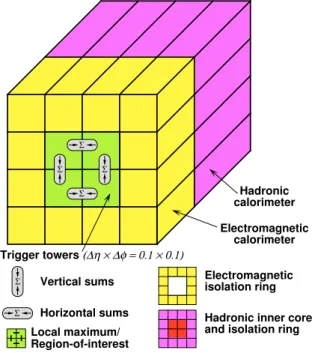
Vertical sums
Σ
Σ Horizontal sums
Σ Σ
Σ
Σ
Electromagnetic isolation ring Hadronic inner core and isolation ring
Electromagnetic calorimeter
Hadronic calorimeter
Trigger towers (∆η × ∆φ = 0.1 × 0.1)
Local maximum/
Region-of-interest
Figure 3.4.: Schema of the trigger algorithm used in the Cluster Processor Module.
taken to avoid multiple counting. The local maximum in such cases is defined as the region where four of the eight possible neighboring windows have equal or less energy deposition while the other four have less energy deposition than the selected region. The local maximum also defines the RoI’s for the electron/photon and τ-triggers.
The Jet/Energy Module (JEM) works with the jet elements which are the sums of 2x2 towers in the EM calorimeters and the hadronic calorimeters behind them. The JEM calculates ET on overlapping windows of sizes 2x2, 3x3 or 4x4 jet elements and compares them to predefined thresholds. Similar to the electron/photon and τ-triggers, multiple counting is avoided by requiring the 2x 2 jet element window to be a local maximum. The same window is defined as the jet RoI. The JEM can compare the results with four PET and eightETmiss thresholds and report results to the CTP.
3.1.1. Level-1 Muon Trigger
The L1 Muon trigger uses the information from the RPC’s in the barrel region and the TGC’s in the end-cap region. The fast response from the RPC’s and TGC’s enables L1 Muon trigger to associate the muon tracks with their corresponding beam-crossings. The L1 Muon trigger checks for muon tracks by looking at the coincidence hits in different chamber layers within a certain path defined by the trigger pT thresholds. Both the


![Figure 2.15.: η dependency of the integrated magnetic field strength for two different azimuthal angles [9].](https://thumb-eu.123doks.com/thumbv2/1library_info/5622937.1692286/31.892.170.637.128.431/figure-dependency-integrated-magnetic-strength-different-azimuthal-angles.webp)