Theoretical investigations of orbital and spin-orbital effects in functionalized graphene

Theoretical investigations of orbital and spin-orbital effects

in functionalized graphene

DISSERTATION ZUR ERLANGUNG DES DOKTORGRADES DER NATURWISSENSCHAFTEN (DR. RER. NAT.) DER FAKULTÄT

FÜR PHYSIK

DER UNIVERSITÄT REGENSBURG

vorgelegt von Susanne Irmer aus

Hirschau

im Jahr 2018

Prüfungsausschuss:

Vorsitzender: Prof. Dr. Dieter Weiss 1. Gutachter: Prof. Dr. Jaroslav Fabian 2. Gutachter: Prof. Dr. John Schliemann Weiterer Prüfer: Prof. Dr. Vladimir Braun

Termin Promotionskolloquium: 13.06.2018

Contents

List of Figures v

List of Tables ix

1 Introduction 1

2 Spin-orbit coupling in graphene systems from symmetry argu-

ments 5

2.1 Spin-orbit coupling in graphene . . . . 5

2.2 Tight-binding model for graphene and effective Hamiltonians . . . . 7

2.3 Spin-orbit coupling from symmetry . . . 11

2.3.1 Microscopic SOC Hamiltonian . . . 11

2.3.2 Symmetry approach . . . 12

2.3.3 Point group symmetries and transformation of spin . . . 13

2.3.4 Practical relations . . . 15

2.4 Spin-orbit coupling under global symmetries . . . 17

2.4.1 Pristine graphene and the point group D

. . . 17

2.4.2 Subgroups of D

. . . 20

2.4.3 SOC and the point group D

. . . 21

2.4.4 SOC and the point group D

. . . 24

2.4.5 SOC and the point group C

. . . 28

2.4.6 SOC and the point group C

. . . 33

2.5 Spin-orbit coupling under local symmetries . . . 37

2.5.1 Local symmetry . . . 37

2.5.2 Adatom in the hollow position . . . 38

2.5.3 Adatom in the top position . . . 40

2.5.4 Adatom in the bridge position . . . 43

2.6 Concluding remarks . . . 46

3 Local spin-orbit coupling from adatoms: Case studies 49 3.1 Adatoms on graphene . . . 49

3.2 Mechanisms for local spin-orbit coupling in graphene . . . 52

3.3 Methods . . . 53

3.4 Methyl functionalized graphene . . . 54

3.4.1 Structure and orbital physics . . . 55

3.4.2 Spin-orbit coupling from dilute methyl coverage . . . 58

3.5 Fluorine functionalized graphene . . . 61

3.5.1 Structure and orbital physics . . . 61

3.5.2 Spin-orbit coupling from dilute fluorine coverage . . . 64

3.6 Copper functionalized graphene . . . 66

3.6.1 Structure and orbital physics . . . 67

3.6.2 Spin-orbit coupling from dilute copper coverage . . . 73

3.7 Concluding remarks . . . 78

4 Adatoms and resonant scatterers in graphene 81 4.1 Resonant scattering in graphene . . . 81

4.2 Methods . . . 83

4.2.1 T -matrix formalism . . . 83

4.2.2 Density of states and momentum relaxation rate . . . 89

4.3 Resonance characteristics for adatoms in the top, bridge, and hollow positions . . . 92

4.3.1 Adatom in the top position . . . 93

4.3.2 Adatom in the bridge position . . . 96

4.3.3 Adatom in the hollow position . . . 98

4.4 Localization of resonant states . . . 102

4.5 Adatoms, vacancies, and the model of a strong midgap scatterer . . 106

4.6 Concluding remarks . . . 110

5 Spin relaxation in bilayer graphene: Resonant scattering off magnetic moments 113 5.1 Spin relaxation in graphene . . . 113

5.2 Spin relaxation by resonant scattering off magnetic moments . . . . 116

5.2.1 Adatom model with exchange . . . 116

5.2.2 Relaxation rates . . . 121

5.3 Is fluorine a magnetic resonant scatterer in graphene? . . . 127

5.3.1 Experiment at Penn State University . . . 128

5.3.2 DFT and TB input . . . 132

5.3.3 Spin relaxation in fluorinated BL and SL graphene . . . 133

5.3.4 Momentum relaxation in fluorinated SL and BL graphene . . 139

5.4 Concluding remarks . . . 142

6 Summary 145

7 Bibliography 149

List of Figures

2.1 Unit cell, Bravais lattice vectors, and Brillouin zone of graphene. . . 8

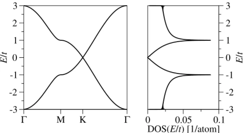
2.2 Band structure and DOS of graphene. . . 10

2.3 Point group symmetry D

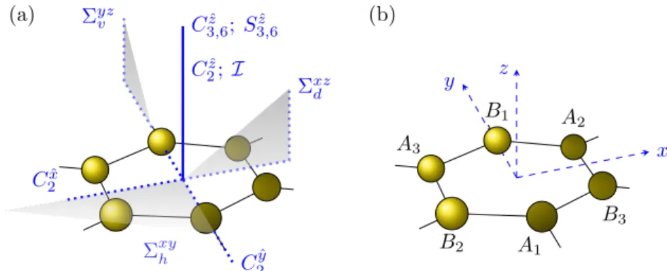
and site labeling convention. . . 13

2.4 Effect of intrinsic SOC on the electronic band structure of graphene. 19 2.5 Electronic band structure and conserved spin quantity around the K point for a D

invariant SOC Hamiltonian. . . 25

2.6 Electronic band structure around the K point for a D

invariant SOC Hamiltonian. . . 27

2.7 Electronic band structure and spin texture around the K point for a C

invariant SOC Hamiltonian. . . 32

2.8 Electronic band structure around the K point for a C

invariant SOC Hamiltonian. . . 35

2.9 Pictorial view of graphene systems with the point groups D

, D

, D

, C

, and C

. . . 36

2.10 Adatom in the hollow position. . . 38

2.11 Adatom in the top position. . . 41

2.12 Adatom in the bridge position. . . 44

3.1 Periodic system of adsorbates studied on graphene. . . 50

3.2 Geometric structure of methyl functionalized graphene and consid- ered supercell. . . 55

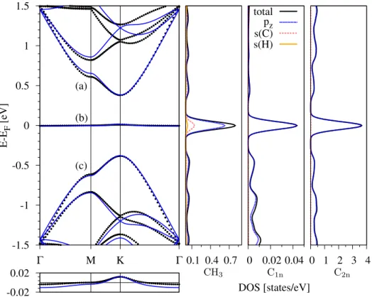
3.3 Electronic band structure and DOS of methyl functionalized graphene with dilute admolecule coverage. . . 56

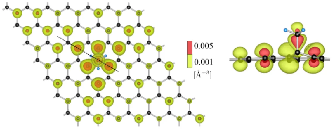
3.4 Electronic charge density of methyl functionalized graphene in the dilute limit. . . 57

3.5 Pictorial view of the local orbital and spin-orbital hoppings describ- ing CH

on graphene in top position. . . 58

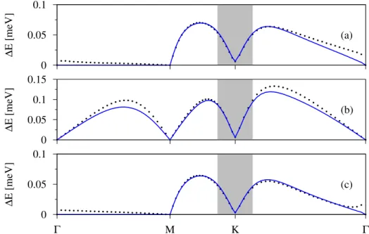
3.6 Spin splitting of bands of methyl functionalized graphene with dilute admolecule coverage. . . 59

3.7 Geometric structure of fluorinated graphene and example for a su-

percell. . . 62

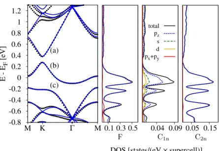
3.8 Electronic band structure and DOS of fluorinated graphene with dilute adatom coverage. . . 62 3.9 Pictorial view of the local orbital and spin-orbital hoppings describ-

ing F on graphene in top position. . . 63 3.10 Spin splitting of bands of fluorinated graphene with dilute adatom

coverage. . . 64 3.11 Schematic view of copper binding in top and bridge position. . . 68 3.12 Electronic band structure of graphene functionalized with copper in

top position for dilute adatom coverage. . . 68 3.13 PDOS of graphene functionalized with copper in top position for a

7 × 7 supercell. . . 69 3.14 Electronic band structure of graphene functionalized with copper in

bridge position for dilute adatom coverage. . . 71 3.15 PDOS of graphene functionalized with copper in bridge position for

a 7 × 7 supercell. . . 72 3.16 Spin splitting of bands of graphene functionalized with copper in top

position with dilute adatom coverage. . . 73 3.17 Spin splitting of bands of graphene functionalized with copper in

bridge position with dilute adatom coverage. . . 75 3.18 Spin splitting of bands of graphene functionalized with copper in top

and bridge position for a 7 × 7 supercell. . . 77 4.1 Convention on unit cell, site labeling, and the nearest neighbor con-

nection vectors, together with the relevant Green’s propagators. . . 87 4.2 Resonance and momentum relaxation characteristics induced by adatoms

in the top position. . . 94 4.3 Resonance and momentum relaxation characteristics induced by adatoms

in the bridge position. . . 97 4.4 Resonance and momentum relaxation characteristics induced by adatoms

(m

= 0) in the hollow position. . . 99 4.5 Comparison of DOS and τ

for different adsorption positions. . . . 100 4.6 Band structure from large supercell for a m

= 0 and m

= 1 orbital

in the hollow position. . . 101 4.7 Resonance and momentum relaxation characteristics induced by adatoms

( m

= 1 ) in the hollow position. . . 103 4.8 Localization of resonant states for adatoms in the top, bridge, and

hollow positions. . . 104 4.9 Signatures of top adatoms in the DOS and τ

in comparison to the

models of a vacancy and the strong midgap scatterer. . . 107

5.1 Band structure and DOS of AB-stacked BL graphene. . . 119

5.2 Electronic band structure of hydrogenated BL graphene. . . 122

5.3 Effect of the exchange coupling on the DOS of hydrogenated SL and BL graphene. . . 123 5.4 Spin and momentum relaxation rates for hydrogenated BL graphene

with local magnetic moments. . . 124 5.5 Scheme of the influence of electron-hole puddles on the spin relax-

ation rates in both hydrogenated SL and BL graphene. . . 127 5.6 Spin relaxation rates for hydrogenated SL and BL graphene with

local magnetic moment. . . 128 5.7 Electronic band structure of fluorinated BL graphene. . . 132 5.8 Effect of the exchange coupling on the DOS of fluorinated SL and

BL graphene. . . 134 5.9 Spin relaxation rate of fluorinated BL graphene. . . 135 5.10 Spin relaxation rate of fluorinated SL graphene. . . 136 5.11 SMS model for the conductivity of SL fluorinated graphene and

hydrogen-like adsorbate induced spin relaxation rate. . . 137 5.12 SMS model for the conductivity of BL fluorinated graphene and

hydrogen-like adsorbate induced spin relaxation rate. . . 138 5.13 Electronic band structures corresponding to the disk scatterer model

in comparison to the DFT results for fluorinated SL and BL graphene.139 5.14 Ratio of spin to momentum relaxation rate in fluorinated SL and BL

graphene. . . 140 5.15 Electronic band structure of fluorinated bilayer graphene including

a finite potential offset to the top layer in the TB calculation. . . . 141 5.16 Ratio of spin to momentum relaxation rate in fluorinated SL and BL

graphene considering fluorine as a charged impurity. . . 142

List of Tables

2.1 Symmetry elements of the point groups D

, D

, D

, C

, and C

. 20 2.2 Orbital tight-binding parameters for the adsorbates hydrogen, methyl,

fluorine, and copper. . . 38 3.1 Orbital and SOC best-fit tight-binding parameters of 5 × 5 and 7 × 7

supercells for methyl functionalized graphene. . . 60 3.2 Orbital and SOC best-fit tight-binding parameters of 7 × 7 and 10 × 10

supercells of fluorinated graphene. . . 66 3.3 Orbital tight-binding parameters and local SOC strengths for graphene

functionalized with the methyl group, fluorine, and copper. . . 78

1 Introduction

In the year 2004, the first exfoliation and characterization of the carbon allotrope graphene [1] heralded a new era of research in the realm of two-dimensional crystal materials. Graphene is a semimetal with its electrons obeying a linear dispersion relation at low energies. As in this energy regime the description of graphene bears resemblance with an effective Dirac equation for massless fermions, this material suggested the possibility to study relativistic effects such as Klein tunneling or zitterbewegung in condensed matter [2].

Graphene offers remarkable qualities regarding its mechanical, optical, thermal and electric properties [3] so that applications of this astonishing material were explored for such diverse topics as flexible electronics [4], chemical sensors [5, 6], or nanopore templates for DNA sequencing [7]. Besides high electron mobilities at room temperature [3], graphene shows a strong ambipolar electric field effect [1]

allowing to tune the charge carrier density in graphene by a gate voltage. Fur- thermore, the sublattice degree of freedom in graphene gives rise to fascinating pseudospin physics and an unconventional integer quantum Hall effect [8, 9].

Bilayer (BL) graphene, two sheets of graphene stacked on top of each other, shares many of the qualities of its single layer (SL) counterpart [10]. However, as BL graphene’s low-energy physics is dictated by a quadratic dispersion relation, also important differences between the BL and SL cases appear, for example, in the form of a third kind of quantum Hall effect [11, 12]. Moreover, the two graphene layers in the BL structure can be addressed separately and a tunable band gap can be introduced by doping or gating [10, 13, 14]. Recently, experimental indications were found that twisted BL graphene exhibits superconductivity [15]. This is a clear difference to SL graphene, where the introduction of superconductivity in the material relies on proximity to superconductors [16–19] and intercalation [20].

Early on, also the research field of spintronics evinced large interest in graphene (SL and BL). This interest was mainly motivated by the negligible hyperfine interac- tion in graphene and its small spin-orbit coupling (SOC) on the order of 10 µeV [21]

due to carbon’s small atomic number

. Long spin relaxation lengths on the scale of µm were found at room temperature [23–28] and the successful injection of spins to

1Carbon has the atomic numberZ = 6. The SOC energy of an electron close to the atomic core can be estimated to scale like SOC∝Z⁴[22].

graphene and its detection were early demonstrated [23, 24, 29, 30], accompanied by large spin signals in the nonlocal resistance of the spin valve experiments [31].

On the other hand, the hope for long spin relaxation times, based on graphene’s small SOC, was not fulfilled. The experimental observations disagree in general with the theoretical predictions by about three orders of magnitude [31–33]. Not only because of this discrepancy but also to realize graphene spintronics devices on the wafer scale, efforts were taken to improve the quality of the graphene sam- ples in order to study spin injection and transport in high-mobility and large-area graphene samples [31].

Spintronics aims to utilize not only the electronic properties of a material but also the spin degree of freedom for fast and efficient memory storage and quantum computing [31]. Therefore, apart the injection and detection of spins, graphene based spintronics devices need to allow for an efficient manipulation of the electron spin.

Both proximitized graphene and graphene functionalized with adsorbates offer ways to manipulate spin and, furthermore, to tailor existing or introduce new feasi- ble properties to graphene, such as superconductivity (see above) and magnetism.

For example, exchange interaction can be induced in the nonmagnetic graphene by placing it on a ferromagnetic insulator [34], or, separated by a tunnel barrier, on a ferromagnetic metal [35]. If also strong SOC is induced, transport magne- toanisotropies [36] are predicted to occur.

Large attention was recently drawn to graphene substrates based on transi- tion metal dichalcogenides (TMDC). These substrates were shown to induce large SOC in graphene giving rise to the spin Hall effect

observable at room tempera- ture [38–41]. This aspect opens the way for spin field effect transistors [42] involving graphene. Also charge-to-spin conversion, relying on the strong Rashba coupling in the TMDC material, was demonstrated experimentally [43] and the occurrence of topological effects in graphene are predicted [44]. The rise of spin-valley locking in graphene on a TMDC allows moreover for optical spin injection into graphene [45–

47]. Recently, giant spin lifetime anisotropy was predicted and demonstrated [48–

50]. The possibility to access and control the relaxation times for different spin orientations proposes graphene-TMDC systems for new spintronics logic devices.

Graphene can be further functionalized locally by adsorbates. Adatoms such as hydrogen [51, 52] and copper enhance graphene’s small intrinsic SOC by factors of 100 (hydrogen) to 1000 (copper) and large spin Hall angles were observed in Refs. [53, 54]. Neutral adatoms with large SOC, such as indium, were predicted to stabilize the quantum spin Hall state in graphene [55]. However, in both the case of the analysis of the spin Hall effect as the experimental verification of the quantum spin Hall state issues remain [56–61].

In this thesis, we concentrate on the theoretical view on both orbital and spin-

2The interested reader can find a review on the spin Hall effect, for example, in Ref. [37].

orbital effects in functionalized graphene, with an emphasis on SOC, the role of specific adsorbates for the latter, resonant scattering off adsorbates, and, finally, a new spin relaxation mechanism for bilayer graphene.

In Ch. 2, we first consider pristine graphene and graphene-like systems which ex- hibit the honeycomb structure. In particular, we take into account two-dimensional lattices described by the point group symmetries D

, D

, D

, C

, and C

, and derive effective SOC Hamiltonians by applying simple symmetry arguments. With this, the ab- or presence of different SOC couplings, such as the well-known intrin- sic one, the Rashba-like coupling, and the PIA term [52], is motivated by intuitive arguments. The second part of this chapter concentrates on SOC in graphene in the presence of the local point group symmetries C

, C

, and C

. These modifi- cations to the local symmetry in graphene are introduced by single adsorbates on the hexagonal lattice in the hollow, the bridge, and the top position, respectively.

Considering the given local changes in the symmetry, we identify and describe the emerging local SOC hoppings in the vicinity of the impurity.

In the following chapter, Ch. 3, we use the insights of the previous chapter and analyze three specific adsorbates on graphene, which are the methyl group, fluorine, and copper. These adsorbates settle down in the top (methyl and fluorine), as well the top and bridge position (copper) on graphene. In order to extract, on the one hand, the local SOC strength and, on the other hand, to identify the microscopic origin of it, we combine tight-binding (TB) models and density functional theory (DFT) calculations.

Chapter 4 is devoted to the orbital impact of hollow, top, and bridge adsorbates with s or p orbital character on scattering resonances in graphene. We choose as a theoretical tool for the investigation the T -matrix approach and complement it with TB calculations of large supercells. This topic has already received large attention throughout the past years due to the prediction of zero-energy states arising, for example, from vacancies. As the density of states (DOS) of pristine graphene vanishes at the charge neutrality point, a strong impact on the orbital quantities such as the conductivity is expected. As we will see in Ch. 5, also the spin relaxation in graphene is largely influenced by adsorbates representing resonant scatterers. In Ch. 4 we concentrate on the orbital aspects of single adsorbates in the three different adsorption positions and the formation of resonance levels. We furthermore compare the case of a general adsorbate to the models of strong midgap scatterers and vacancies and outline the differences between them.

Spin relaxation in graphene and a possible mechanism to explain the observed

difference in magnitude between theory and experiment are the topic of Ch. 5. We

first explain a new spin relaxation mechanism which relies on resonant scattering

off magnetic moments in SL [62] and BL graphene. These local magnetic moments

are likely introduced in small concentrations in experimental graphene samples due

to vacancies or contaminating adsorbates such as hydrogen or methyl. We concen-

trate in particular on BL graphene and find that an hydrogen amount of about

1 ppm is sufficient to recover the experimental spin relaxation data of Refs. [26, 27]. The distinct dependence of the spin relaxation rate on the charge carrier den- sity observed in SL and BL graphene samples can be explained by the presence of electron-hole puddles. In the second part, the focus lies on fluorinated SL and BL graphene as fabricated and measured in the group of Jun Zhu at Penn State University. By applying our spin relaxation model, which is supported by DFT cal- culations of fluorine, we aim to resolve the theoretical debate on whether fluorine induces local magnetic moments in graphene or not. We report here on the current status of this ongoing project and present the discrepancies found so far between the experimental observations and our model predictions.

The results of this thesis are summarized in Ch. 6.

2 Spin-orbit coupling in graphene systems from symmetry arguments

This chapter is based on the paper “Model spin-orbit coupling Hamiltonians for graphene systems”, PRB 95, 165415 (2017), by Denis Kochan, Susanne Irmer, and Jaroslav Fabian.

2.1 Spin-orbit coupling in graphene

The first theoretical description of the electronic band structure of graphene goes back to the work of Philip R. Wallace in 1947 [63]. Neglecting the coupling between graphite’s single layers, he essentially derived a TB model for graphene. Further- more, he showed that the conduction and valence band touch at the six corners of the Brillouin zone, the K points, which makes graphene a semimetal. In the fifties and the following years, the attention was drawn to the effect of SOC in graphene.

Slonczewski [64], McClure and Yafet [65], and Dresselhaus and Dresselhaus [66]

argumented on a group theoretical basis that the SOC intrinsic to graphene in- troduces a gap at the corners of the Brillouin zone. However, it took about fifty years to obtain realistic estimates for this spin-orbit gap. Intense studies on the SOC of graphene had been resumed after graphene’s exfoliation in 2004 [1]. Kane and Mele [67] revived the studies in 2005 by estimating the spin-orbit gap ∆

to be about 200 µeV. This was a promising prediction since it inferred that the quan- tum spin Hall state should be observable in graphene at low temperatures of a few Kelvins.

In the subsequent years, it was shown by several groups that the value of ∆

had been significantly overestimated in Ref. [67] by a factor of 10-100. Specifically, the contribution of the mixing of σ and π states to the SOC is very weak and of the order of 1 µeV [21, 68–70]. The low energy states of graphene, i.e., the occupied states forming the π bands around the K points, are mainly built from the 2p

orbitals of the carbon atoms. These p

orbitals, having zero magnetic quantum

number, have to couple to states with nonzero magnetic quantum number in order

to induce a finite SOC gap at K . Possible candidates are the p

and p

orbitals of

the σ band, or orbitals with even higher magnetic quantum number such as the d

orbitals.

In flat graphene, the p

orbitals are orthogonal to the p

and p

orbitals. How- ever, the intra-atomic SOC allows for a spin-flipping hopping of electrons between the p

and the p

or p

orbital on the same carbon atom. It can be shown by group theoretical arguments (see for example Sec. 2.4.1) that the intrinsic SOC of graphene is described by an overall spin-conserving hopping process, which couples next-nearest neighbor carbon atoms. Therefore, the spin-orbit gap will depend in leading order on the square of the spin-flip hopping strength between the p lev- els [21, 68–71]. Although the spin-orbit splitting of the 2p states (entering the σ band) of an isolated carbon atom is about ∆

≈ 10 meV [21, 67], the spin-orbit gap at the K points resulting from this σ - π mixing process

is in total only of the order of 1 µeV [21, 71].

The importance of the d orbitals for the SOC in graphene was already pointed out by Slonczewski [64] and McClure and Yafet [65]. Indeed, the states around the Fermi level show a small contribution of the unoccupied 3d

and 3d

levels of carbon [21]. This allows for a direct overlap between the p

and d

or d

states on neighboring carbon atoms in graphene. The atomic SOC between d

and d

is of spin-conserving nature and, therefore, contributes in the first order to the intrinsic SOC of graphene. Although the atomic SOC hopping strength between the d orbitals is smaller than the one between the p orbitals, the small but direct overlap of the p

and d states on the neighboring carbon atoms is important and the d levels cause about 96% of the spin-orbit gap observed in the DFT calculations of Gmitra et al. [21]. The gap opened at the K points was found in this work to be about 24 µeV. In an earlier DFT work, Boettger and Trickey [72], who employed a different approximation for the treatment of the SOC, found a gap of about 50 µ eV. In the rest of this thesis, we will consider the spin-orbit gap of 24 µ eV as the reference value for the intrinsic SOC gap in graphene.

Placing graphene in an external electric field or on a substrate, a so-called Rashba SOC emerges in the graphene system. This coupling is of extrinsic nature and, thus, can be tuned by modifying the external conditions, for example by changing the electric field strength. The Rashba SOC is described as a spin-flipping hopping be- tween nearest carbon neighbors and causes a spin splitting of the otherwise twofold degenerate bands of graphene. The microscopic origin of the Rashba coupling is found in the σ-π mixing in combination with the atomic Stark effect [21, 68, 69, 71]

which couples the s orbital with the p

orbital within the same carbon atom. The d orbitals are of less importance for the magnitude of the Rashba coupling [21, 71].

Gmitra et al. [21] found in their DFT study that the Rashba strength grows lin- early with the electric field strength, yielding the value of 5 µ eV for typical electric field strengths of 1 V/nm. Previously, Kane and Mele [67] estimated the Rashba

1Explicitly, Konschuhet al. [71] find that theσ-π mixing contribution to the spin-orbit gap is 4 (∆p/3)²(εp−εs)/(9V_spσ² ). From a DFT analysis, they obtain for the difference of the on-site energies of thes andporbitals |εp−εs| ≈10eV and for the overlap parameterVspσ ≈6eV.

This leads to the spin-orbit gap magnitude of1µeV considering onlyσ-πmixing.

2.2 Tight-binding model for graphene and effective Hamiltonians

coupling to be an order of magnitude smaller, while other works [68, 69] predicted it to be one order of magnitude larger compared to the DFT result of Gmitra et al. [21].

Modifications to graphene’s crystal structure directly affect the SOC, both in strength and in the underlying origin or mechanism. Proximity effects from differ- ent substrate materials [45, 73–76], for example, can transfer strong SOC to the graphene band structure. Furthermore, curvature effects [21, 68] are well-known from the SOC studies of carbon nanotubes and are predicted to enhance the effect of σ - π mixing by an order of magnitude [68] in undulating graphene [77–79]. Lo- cally, adsorbates binding to graphene [51] can also lead to a notable enhancement of the SOC of about a factor of 10 to 100 through sp

distortion in the σ network of graphene [51]. As another mechanism, depending on the adsorbate, also the intra-atomic SOC of the impurity can locally influence the SOC strength, see for example Ch. 3.

In this chapter, we concentrate on the SOC in graphene systems, i.e., systems with a hexagonal honeycomb structure under specific global and local structural modifications. The structural modifications reduce the point group symmetry of the system and can, therefore, give rise to new SOC mechanisms. Explicitly, we study in the first part of this chapter the point groups D

, D

, D

, C

, and C

. In the second half, we focus on local adsorbates binding in the hollow, top, and bridge positions and the allowed SOC hoppings in the vicinity of the impurity.

Examples of adatoms together with realistic estimates of the local SOC strength will be treated in Ch. 3. We close the chapter with a short summary and a comparison to the approach and results of three other works [55, 80, 81] on the impact of adsorbates on graphene’s SOC.

2.2 Tight-binding model for graphene and effective Hamiltonians

Graphene and the graphene systems, which we will consider in the following sec- tions, have a hexagonal lattice structure with a two-atomic basis. Equivalently, the lattice structure can be described by two interpenetrating hexagonal sublattices (each with a one-atomic basis) labeled by A and B, which form the well-known honeycomb lattice. Figure 2.1(a) shows our choice of the unit cell together with three Bravais lattice vectors

R

= a

cos

, sin

, α = 1, 2, 3 , (2.1)

where a

is the lattice constant. In graphene we have a

= 2.46 Å. Selecting for

the two primitive translation vectors R ˜

= R

and R ˜

= − R

, we obtain the basis

R1

A R2

B R3

(a) G2

G1

Γ +K

−K

M (b)

Figure 2.1:

(a) Unit cell of the hexagonal graphene lattice with the two-atomic basis

and

and the Bravais lattice vectors

(α

graphene with the reciprocal lattice vectors

and the high symmetry points

,

and

(τ

).

vectors of the reciprocal lattice, G

= 4π

√ 3a

cos

, sin

, α = 1, 2 , (2.2)

which obey the orthogonality relation G

. R ˜

= 2πδ

. The corresponding max- imally symmetric unit cell in reciprocal space, the first Brillouin zone, is shown Fig. 2.1(b). The first Brillouin zone contains the high symmetry points Γ , M , and τ K , which are invariant under specific subgroups of the full point group describing the direct lattice. The points Γ and M are the so-called time reversal symmetric points, as their time reversal counterparts differ only by a reciprocal lattice vector

. The points τ K (τ = ± ) are defined as the corners of the Brillouin zone and result from the two sublattices A and B. In graphene, they are also known as the Dirac points or Dirac valleys. The term “Dirac” is borrowed from the famous relativistic Dirac equation: Around the two τK points, graphene’s dispersion is linear and can be described by a relation that looks similar

to the Dirac equation in the limit of zero mass.

The low-energy physics of graphene is well-described within a TB description based on π orbitals. The TB method, which is closely related to the LCAO method from chemistry, describes single-electron states which are localized at the atomic sites in the crystal lattice so that their wave functions reflect the atomic orbital of the ion. Leaving SOC aside for this moment, the Hamiltonian describing the orbital motion of an electron in the crystal lattice is given by

H ˆ

= − ~

2m ∇

+ V

(r) + X

i6=0

v

(r) . (2.3)

2The time reversal symmetry is introduced in Sec. 2.3.3 and its influence on the spectrum is shortly commented in Sec. 2.4.1

3With this analogy one has to keep in mind that the itinerant electrons in graphene are not relativistic. Their Fermi velocity is about10⁶m/s.

2.2 Tight-binding model for graphene and effective Hamiltonians

The second and third term in the Hamiltonian build the crystal potential which is formed of the potential of the ionic site hosting the electron, V

, and the contribution of the remaining ionic sites and electrons, P

i6=0

v

(r). We choose the basis to be composed of single (real-valued) π -orbital states | X

σ i with spin σ per lattice site n and take the matrix elements of H ˆ

with all possible combinations of | X

σ i . Neglecting the overlap of atomic orbitals on different lattice sites, h X

σ | X

σ

i ≈ δ

δ

, two kinds of terms appear: the on-site energy on lattice sites n , represented by the matrix element h X

σ |−

∇

+V

(r − r

) | X

σ i, and the hopping integrals, h X

σ | P

i6=0

v

(r − r

) | X

σ i, connecting sites n and m. We determine our reference zero energy by setting the on-site energy of all π -orbitals to zero. Furthermore, we neglect all hopping integrals going beyond nearest neighbor contributions

. Within this nearest neighbor approximation, the orbital TB Hamiltonian for graphene reads

H

= − t X

σ

X

hm,ni

X

σ X

σ

, (2.4)

where the positive quantity t is the nearest neighbor hopping strength, for which one finds in the literature for graphene a value of about 3 eV [3, 71, 82]. Throughout this thesis, we fix the nearest neighbor hopping strength to t = 2.6 eV. To obtain the band structure of graphene, we transform H

from the local atomic into the Bloch basis, | X

σ i → | X

σ i ,

X

σ

= 1

√ N X

Rm

e

X

σ

. (2.5)

Here, we set X ∈ { A, B } according to the sublattice of the site and measure the quasi-momentum q from the center of the hexagonal Brillouin zone at the Γ point.

The number of graphene unit cells enters Eq. (2.5) as the quantity N . Note that R

is the lattice vector pointing to the m-th unit cell that hosts the orbital | X

σ i . We can now express the orbital Hamiltonian in the Bloch form, H

= P

q

H

(q), with

H

(q) = − t X

σ

f

(q) ˆ s

σσ

A

σ B

σ

+ H.c. , (2.6) where s ˆ

represents the unit matrix in spin space (see below) and the orbital struc- tural function is given by

f

(q) =

1 + e

+ e

. (2.7) Diagonalizing Eq. (2.6), we obtain the dispersion relation for the π states of graphene which form the conduction ( n = +1 ) and the valence band ( n = − 1 ),

(q) = n t | f

(q) | . (2.8)

Γ M K Γ -3

-2 -1 0 1 2 3

E/t

0 0.05 0.1

DOS(E/t) [1/atom]

-3 -2 -1 0 1 2 3

E/t

Figure 2.2:

(a) Band Structure of graphene with the linear dispersion around the

point and, (b), corresponding DOS of graphene.

Figure 2.2 shows the energy dispersion of graphene in momentum space resulting from the diagonalization of Eq. (2.4) together with the DOS

.

In pristine (undoped) graphene, the Fermi level lies at zero energy, i.e., it crosses the energy dispersion directly at the Dirac points where the valence and conduction band meet. The linear dispersion, which appears at nearby energies, can be further investigated by considering quasi-momenta q = τK + k around the Dirac point

τ K = τ 4π 3a

(1, 0) . (2.9)

Keeping the first nonzero term in the expansion of Eq. (2.7) in k , we obtain f

(τK + k) '

√ 3a

2 − τ k

− ik

, (2.10)

and the orbital Hamiltonian, Eq. (2.6), reduces in the low-energy limit to H

(τK + k) = ~ v

τ k

σ ˆ

− k

σ ˆ

s ˆ

. (2.11)

Here, we introduced the Fermi velocity v

= √

3a

t/2 ~ which has for graphene the value of about v

≈ 10

m/s. The sublattice degree of freedom is described by the Pauli matrices ˆ σ

acting on the sublattice space, whereas for the spin degree of freedom we use the Pauli matrices ˆ s

in the spin space. We choose as the ordering of the sublattices { A, B } and for the spins σ = {↑ , ↓} with spin quantization axis along z . The spin-Pauli matrices are given by

ˆ s

=

1 0 0 1

, ˆ s

=

0 1 1 0

, s ˆ

=

0 −i i 0

, s ˆ

=

1 0 0 − 1

(2.12)

4The next-nearest neighbor hopping term, for example, induces electron-hole asymmetry in the spectrum of graphene.

5For the diagonalization, the LAPACK [83] routine zheevx is employed. The DOS is calculated applying the triangle method [84] for the integration over the two-dimensional Brillouin zone.

2.3 Spin-orbit coupling from symmetry

and are equivalently defined for the sublattice degree of freedom, for example [ˆ σ

]

= 1 = − [ˆ σ

]

and [ˆ σ

]

= 0 = [ˆ σ

]

. The linear dispersion relation appears then after diagonalizing Eq. (2.11) and reads

(τK + k) = n ~ v

| k | . (2.13) In graphene, the π-orbitals are primarily built of the carbon 2p

orbitals, though all TB and symmetry discussions of the following sections are valid for any atomic orbital with quantum numbers n , l 6 = 0 , m

= 0 . We further note that for hexagonal systems other than pristine graphene the value of t might differ and its magnitude needs to be re-estimated or fitted for a quantitative analysis of those systems.

Additional terms in Eq. (2.4) can arise if A and B sublattice atoms are distinct or feel different electrostatic potential; see the examples of planar hexagonal boron nitride (hBN), Sec. 2.4.4, or graphene on a TMDC, Sec. 2.4.6.

In the subsequent sections we focus on the following question: Given a graphene system (and its point group symmetry) what can we predict for the SOC? Concen- trating on the modeling site of this problem, we will derive effective Hamiltonians describing the spin-degree of freedom in the structure. We consider one effective orbital per lattice site from which we demand invariance under certain symmetries.

The approach is symmetry based which enables us to make general statements for different structural realizations of graphene systems with the same point group symmetry and provides us with a first intuitive view on the subject. The effective description incorporates the microscopic origin of the SOC but does not rely on a detailed description of the SOC in the vicinity of the atomic cores. The study of specific systems may call in a second step for multi-orbital TB models, e.g. in the Koster-Slater two-center approximation, and, for a quantitative analysis of the spin-orbit strength, DFT calculations. The effective SOC Hamiltonians for the local adsorbates will be applied to three specific impurities in Ch. 3, which also supports the validity of our following statements.

2.3 Spin-orbit coupling from symmetry

2.3.1 Microscopic SOC Hamiltonian

SOC appears as a relativistic correction in the Schrödinger equation at the atomic level and can be directly observed in the fine structure of atomic spectra. It de- scribes the coupling of an electron’s momentum to its spin degree of freedom as it moves under the influence of the gradient of an electric potential. For atoms in a lattice, the potential is represented by the effective crystal field potential V . The Hamiltonian for this microscopic spin-orbit interaction is given by

H ˆ

= ~

4m

c

∇V × p ˆ

.ˆ s , (2.14)

where m is the vacuum rest mass of the electron, c the speed of light, p ˆ the mo- mentum operator, and s ˆ = (ˆ s

, ˆ s

, s ˆ

) represents the array of Pauli matrices acting on the spin degrees of freedom. For the discussions below, it is useful to expand the Hamiltonian in spin-raising and spin-lowering operators, s ˆ

= ˆ s

± iˆ s

,

H ˆ

= ˆ L

s ˆ

+ ˆ L

ˆ s

+ ˆ L

s ˆ

. (2.15) The L’s are differential operators which act only on the orbital part of the wave ˆ function

.

2.3.2 Symmetry approach

Starting point for the derivation of an effective, system-specific SOC Hamiltonian is the system’s (local) symmetry which is described by a set of symmetry operations and their respective representations S. The symmetry allows or forbids certain spin-orbit mediated hopping terms between lattice sites. Thus, we need to inves- tigate the behavior of the matrix elements

X

σ | H ˆ

| X

σ

of the microscopic SOC Hamiltonian under symmetry in our effective one-particle Hilbert space. As the gradient of the crystal field potential ∇ V is largest around the atomic cores, the magnitude of the matrix elements decreases strongly with increasing distance between sites n and m. Our analysis of SOC mediated hoppings is therefore re- stricted to on-site, nearest neighbors, and next-nearest neighbors. Let us first give general relations that will facilitate our SOC studies.

If the system’s structure is invariant under a symmetry operation S (S is a group element of the structure’s point or space group) then both orbital and spin-orbital Hamiltonian have to commute with S . In particular, this means that the effective SOC matrix element between states | X

σ i and | X

σ

i fulfills

for unitary S

S [X

σ] | H ˆ

| S [X

σ

]

=

S [X

σ] | S [ ˆ H

X

σ

]

=

X

σ | H ˆ

| X

σ

. (2.16)

We further impose time reversal T symmetry on our systems which is represented by an antiunitary operator and can therefore be written as the product of a uni- tary operator and complex conjugation. From this follows directly how the matrix

6The operatorsLˆ transform under space and time reversal symmetry as the standard angular momentum operatorsLˆ but do not fulfill their SU(2)-commutation relations. In a microscopic treatment of the SOC, the SOC is most efficient in the vicinity of the atomic core. There, the crystal field potential can be approximated by the spherically symmetric atomic potential.

With V(r) = V(|r|) and ∇V = (r/r)(dV /dr), the Hamiltonian of Eq. (2.14) reduces to Hˆso=ξ(r) ˆL.ˆs[85]. The factorξ(r)incorporates all of the radial information.

7We employ the notation|αS[Xnσ]

≡αS|Xnσ

to denote a state|Xnσ

after transformation under the operationαS.

2.3 Spin-orbit coupling from symmetry

C_3,6^zˆ ; S_3,6^zˆ C₂^zˆ; I Σ^yz_v

C₂^yˆ Σ^xz_d

C₂^xˆ

Σ^xy_h (a)

x y z

A3

B2

B1

A1

A2

B3

(b)

Figure 2.3:

(a) Symmetries of the point group

, which leave the honeycomb lattice structure invariant. (b) Chosen coordinate system and labeling of the carbon sites on one hexagon ring.

elements for the self-adjoint Hamiltonian transform under time reversal symmetry

, T [X

σ] | H ˆ

| T [X

σ

]

=

T [X

σ] | T [ ˆ H

X

σ

]

=

X

σ | H ˆ

| X

σ

=

X

σ

| H ˆ

| X

σ

. (2.17)

2.3.3 Point group symmetries and transformation of spin

We have to specify from which pool of symmetries we can select S . Pristine graphene is invariant under the crystallographic point group

D

, which comprises the 24 group elements of unity E , rotations C

, space inversion I, reflections Σ and improper rotations S

in 12 classes,

D

= { E; 2C

; 2C

; C

; 3C

; 3C

; I ; Σ

; 3Σ

; 3Σ

; 2S

; 2S

} . (2.18) Here, each class is represented by one symmetry operation and the numbers in front specify the total number of equivalent elements contained in the respective class. Representative operations of each class are shown in Fig. 2.3(a) and we use the following notation: Superscripts xy , yz , and xz identify the location of reflection planes in our coordinate system, which is shown in Fig. 2.3(b), and we add for emphasis the attributes horizontal (h), vertical (v), and diagonal

(d), respectively. Superscripts x ˆ , y ˆ , and z ˆ specify the axes of spatial rotations. The

8By awe denote the complex conjugate of the quantitya.

9We label the point groups according to the Schönflies notation [86].

10This plane is commonly called a dihedral plane since it contains the principal axis (axis with highest rotational symmetry) and bisects the angle between twoC2axes that are perpendicular to the principal axis [86].

angle of rotation Φ

= 2π/l is encoded in the subscript l . Apart of proper rotations C

, D

also contains improper rotations S

, which involve a proper rotation, C

, followed by reflection about the horizontal plane, Σ

. Note that the π-orbitals are odd under horizontal reflections, inversion, and π -rotations around in-plane axes.

Throughout the first part of this chapter we will study and compare SOC in systems with the point group D

and its subgroups D

, D

, C

, and C

. Depending on the system, we will apply only a subset of the symmetry operations contained in D

.

For our spin-orbit analysis we further need to know, how spin ↑ and ↓ components transform under a symmetry operator S. With the help of the unit matrix and the spin-Pauli matrices, one can write down a two-dimensional representation of the operator for rotation of spin by angle Φ

around the axis n ˆ

[22],

C

= e

= cos Φ

2

− i n ˆ

.ˆ s sin Φ

2

, (2.19)

and reflection of spin in a plane with plane normal n ˆ

,

σ

= − i n ˆ

. s ˆ . (2.20)

Specifically, we choose for the reflection planes xy, yz, and xz the plane normals ˆ

n

pointing along the (positive) cartesian axes α displayed in Fig. 2.3(b).

For one-particle spin-

/

states, the time reversal operator fulfills T

= − 1 [86].

We choose as a specific representation for the anti-unitary operator T = − iˆ s

C ˆ where C ˆ indicates complex conjugation. As we are considering real (effective) or- bitals the time reversal operator only affects the spin part of the wave function.

We can now write down transformation rules for our π-orbital states | X

σ i under the symmetry operations S presented in Fig. 2.3(a), time reversal T and translations T

along ~a,

| X

σ

−−→ e

| X

l(m)

σ

, (2.21a)

| X

σ

−−→ i | X

2(m)

( − σ)

, (2.21b)

| X

σ

ˆ y

−−→

( − 1)

| X

2(m)

( − σ)

, (2.21c)

| X

σ

xy

−−→

i( − 1)

| X

σ

, (2.21d)

| X

σ

−−→ − i | X

( − σ)

, (2.21e)

| X

σ

−−→ ( − 1)

| X

( − σ)

, (2.21f)

| X

σ

−−→ i( − 1)

e

| X

l(m)

σ

, (2.21g)

| X

σ

−−→ ( − 1)

| X

( − σ)

, (2.21h)

2.3 Spin-orbit coupling from symmetry

| X

σ

−−→ −| X

σ

, (2.21i)

| X

σ

−−−→ | X

σ

. (2.21j)

The transformation properties under improper rotations follow directly from S

= Σ

◦ C

and we can rewrite space inversion as I = Σ

◦ Σ

◦ Σ

.

Equivalently, we could do our symmetry analysis in the space of quasi-momenta by transforming the local atomic basis | X

σ i to the Bloch basis | X

σ i. One obtains similar transformation rules as in Eqs. (2.21) where it has to be taken into account that both time reversal and inversion cause q 7→ − q . We focus in our symmetry analysis on the states in Wannier space as we will discuss both systems with and without translational symmetry (Sec. 2.4 and Sec. 2.5, respectively). In the first case we will express our effective SOC Hamiltonians also in the Bloch basis to show the impact of the SOC terms on the band structure at low energies.

2.3.4 Practical relations

Time reversal symmetry and the properties of H ˆ

, Eq. (2.15), alone provide already important information about the nature of SOC terms in graphene-like systems.

Time reversal symmetry, for example, connects SOC matrix elements with opposite spin projections,

X

σ H ˆ

X

σ

=

(2.21h)

=

( − 1)

T [X

( − σ)]

H ˆ

( − 1)

0

2

T [X

( − σ

)]

= − ( − 1)

0

2

T [X

( − σ)]

H ˆ

T [X

( − σ

)]

(2.17)

= − ( − 1)

0

2

X

( − σ

) H ˆ

X

( − σ)

. (2.22)

We will exploit this relation frequently in our SOC analysis. In particular, it follows that on-site spin-flipping SOC terms, i.e., n = m and σ

= − σ , are equal to zero:

X

σ H ˆ

X

( − σ)

= − X

σ

H ˆ

X

( − σ)

. (2.23)

Furthermore, as σ

s ˆ

σ

= 0 , Eq. (2.15) indicates that a spin-conserving hop- ping changes sign under an overall flip of the spins,

X

σ H ˆ

X

σ

= −

X

( − σ) H ˆ

X

( − σ)

. (2.24)

Getting time reversal symmetry involved in the game, we find X

( − σ)

H ˆ

X

( − σ)

= X

σ

H ˆ

X

σ

= X

σ

H ˆ

X

σ

, (2.25)

which, together with Eq. (2.24), implies that a spin-conserving SOC term coupling sites n and m is purely imaginary. Though, in the case of n = m we see that

X

σ H ˆ

X

σ

=

X

( − σ) H ˆ

X

( − σ)

(2.24)

= − X

σ

H ˆ

X

σ

. (2.26)

Thus, on-site spin-conserving SOC terms vanish for all sites m.

So far, we have not used any point-group specific symmetries. As we will see in the following, we can make three statements about the absence of SOC terms related to the presence of specific symmetries. In detail, the statements explain why we find for pristine graphene, point group D

, only the intrinsic SOC term.

Statement 1. Spin-flipping SOCs are inhibited by horizontal reflection Σ

. With a glance at Eq. (2.21d), we write

X

σ H ˆ

X

( − σ)

(2.21d)

=

i( − 1)

Σ

[X

σ]

H ˆ

i( − 1)

Σ

[X

( − σ)]

= −

Σ

[X

σ]

H ˆ

Σ

[X

( − σ)]

(2.16)

= − X

σ

H ˆ

X

( − σ)

, (2.27)

which is fulfilled only if X

σ

H ˆ

X

( − σ)

= 0 .

Statement 2. Nearest neighbor spin-flip SOCs are inhibited by a combination of space inversion I , translation T

, and time reversal T .

We show the effect of the symmetries, as an example, on one matrix element h A

σ

H ˆ

B

( − σ) i [see Fig. 2.3(b)]. All other nearest neighbor spin-flip matrix elements can be treated analogously. Under space inversion and translation along

~a = −−−→

A

A

= −−−→

B

B

the matrix element transforms to A

σ

H ˆ

B

( − σ)

=

−I [B

σ]

H ˆ

− I [A

( − σ)]

=

I [B

σ]

H ˆ

I [A

( − σ)]

(2.16)

= B

σ

H ˆ

A

( − σ)

(2.21j)

=

T

[B

σ]

H ˆ

T

[A

( − σ)]

(2.16)

= B

σ

H ˆ

A

( − σ)

. (2.28a)

The right side of Eq. (2.28a) is distinct from the initial matrix element by complex conjugation and interchange of spin. This calls for applying time reversal symmetry,

B

σ H ˆ

A

( − σ)

= − A

σ

H ˆ

B

( − σ)

, (2.28b)

2.4 Spin-orbit coupling under global symmetries

and thus we showed that the nearest neighbor SOC mediated spin-flip hopping is zero due to the presence of space inversion, translation, and time reversal.

Statement 3. Nearest neighbor spin-conserving SOCs are inhibited by a combina- tion of vertical reflection Σ

and translation T

.

We first translate the states | A

σ i and | B

σ i along ~a = −−−→ A

A

= −−−→ B

B

and go back to the initial position by Σ

, i.e.,

A

σ H ˆ

B

σ

=

A

σ H ˆ

B

σ

(2.21e)

=

iΣ

[A

( − σ)]

H ˆ

iΣ

[B

( − σ)]

=

A

( − σ) H ˆ

B

( − σ)

(2.29a) With help of Eq. (2.24) we finally obtain, in accordance with our third statement,

A

σ H ˆ

B

σ

= − A

σ

H ˆ

B

σ

= 0 . (2.29b)

When we consider subgroups of D

, i.e., we explicitly lower the symmetry in our system, certain symmetry operations are absent and, thus, specific statements are not fulfilled. In particular, the third statement does not necessarily hold in the case of local adsorbates where translational invariance is absent. We will nevertheless first consider systems with translational invariance.

2.4 Spin-orbit coupling under global symmetries

2.4.1 Pristine graphene and the point group D

In the previous section we showed that the π-states in D

invariant graphene me- diate only a next-nearest neighbor spin-conserving SOC term. This is the so-called intrinsic SOC and we will label its strength by λ

. It enters the SOC Hamiltonian as

H

= iλ

3 √ 3

X

σ

X

hhm,nii

ν

ˆ s

σσ

X

σ X

σ

. (2.30)

Here, the summation over hh m, n ii addresses all second nearest neighbor sites m and n which are members of the same sublattice. By convention, the SOC strength λ

enters Eq. (2.30) with the numerical prefactor (3 √

3)

which simplifies the form of

the low-energy expansion in Bloch space (see below). The imaginary unit i reflects

the purely imaginary nature of spin-conserving hoppings in graphene, Eqs. (2.24)

and (2.25). As seen before in Eq. (2.24), the intrinsic SOC comes with opposite sign