Spin relaxation in s-wave superconductors in the presence of resonant spin-flip scatterers

(1)

SUPPLEMENTAL MATERIAL

Spin relaxation in s-wave superconductors in the presence of resonant spin-flip scatterers

Denis Kochan, Michael Barth, Andreas Costa, Klaus Richter, and Jaroslav Fabian Institute for Theoretical Physics, University of Regensburg, 93040 Regensburg, Germany

The following Supplemental Material presents in detail spin-relaxation fundamentals in connection to analytical T-matrix approach, and, primarily, to its superconduct- ing Kwant-package implementation. The last section dis- cusses the break-down of the Hebel-Slichter effect in res- onant Josephson junctions, what provides an evidence that the effect is more universal and extends beyond su- perconducting graphene.

Spin relaxation of quasiparticles (QPs) in the su- perconducting phase depends on the underlying scat- tering mechanism, namely its time-reversal parity [S1].

The latter determines how the electron and hole tran- sition amplitudes combine giving rise to the final spin- flip rate. As pointed out by Yafet [S2], the spin relax- ation rate in the superconducting phase, 1/τ

_s^SC

, relates—

within first-order perturbation theory—to its normal- phase counterpart, 1/τ

_s^N

, by

1/τ

_s^SC

∼ h(u

k

u

_q

± v

_k

v

_q

)

²

/τ

_s^N

i. (S1) Here, u and v are the standard BCS coherence factors of the QP wave functions participating in scattering, and h· · · i represents thermal broadening over the QP ener- gies. Consequently, the spin relaxation rate in the su- perconducting phase increases or decreases depending on the relative sign between the coherence factors. The plus (minus) sign applies to perturbations that are odd (even) w.r.t. time-reversal symmetry, e.g., magnetic im- purities (local SOC fields), eventually giving rise to a larger (smaller) 1/τ

_s^SC

compared to 1/τ

_s^N

. As demon- strated in the main text for superconducting graphene, those differences vary with the chemical potential and temperature, and can even change by a few orders of magnitude. Thus conducting the same spin relaxation measurement in the normal and superconducting phase of graphene, and comparing 1/τ

_s^N

to 1/τ

_s^SC

would provide an unprecedented experimental feasibility to disentangle the dominant spin relaxation mechanism.

The qualitative physical understanding is rather in- tuitive. On the one hand, QPs have well-defined spins and almost the same mass as normal-phase carriers, but energy dependent effective charges q = (u

²

− v

²

) e

_el.

, es- pecially for QPs in the coherence peaks (u

²

' v

²

) that dominate scattering at T < T

_c

. Therefore, ‘direct charge- charge’ interaction is less pronounced (superconducting pairing enfeebles Coulomb repulsion) and the ‘indirect spin-spin exchange’ takes over, giving 1/τ

_s^SC

> 1/τ

_s^N

. This effect is known as Hebel-Slichter effect [S3–S5]. On

the other hand, not only the QP charges diminish, but also their group velocities v

_SC

' |(u

²

− v

²

)| v

_N

and like- wise their momenta. Since spin-orbit coupling (SOC) couples QP spins to their momenta

SOC

_SC

≈ m(v

_SC

× L) · s ≈ |(u

²

− v

²

)| m(v

_N

× L) · s

| {z }

SOCN

,

the effective SOC strength significantly decreases in the superconducting phase, implying 1/τ

_s^SC

< 1/τ

_s^N

.

SPIN-ORBIT COUPLING HAMILTONIAN In the main text, we use the local SOC Hamiltoni- ans V

s⁽²⁾

that capture spatially localized spin-orbit fields adatoms induce in graphene. Those tight-binding model Hamiltonians are based on relevant local symmetries [S6]

and their couplings are fitted to first-principles calcula- tions; see Ref. [S7] for more details regarding hydrogen and Ref. [S8] for fluorine.

Since the SOC of pristine graphene is weak, about 40 µeV [S9], it does not play a significant role, and we disregard that global SOC contribution. The de- fect region in our model consists of the adatomized car- bon (site m = 0) and its three nearest (nn), C

nn

, and six next-nearest (nnn), C

nnn

, neighbors. A minimal effective SOC Hamiltonian in local atomic basis that is consistent

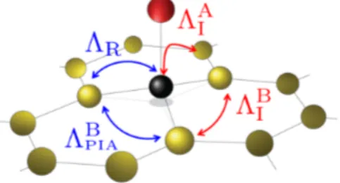
FIG. S1. Schematic representation of the local SOC strengths

in the vicinity of the adatom (red), which eventually enter

the SOC Hamiltonian V

s⁽²⁾

. Blue and red arrows label spin-

flipping and spin-conserving SOC hoppings, connecting spe-

cific nearest or next-nearest neighbor carbon atoms (yellow).

(2)

II with the local symmetries reads then as

V

_s⁽²⁾

= iΛ

^A_I

3 √

3 X

m∈Cnnn

X

σ

c

^†_0σ

(ˆ s

z

)

_σσ

c

_mσ

+ h.c.

+ iΛ

^B_I

3 √

3 X

m,n∈Cnn m6=n

X

σ

c

^†_mσ

ν

_mn

(ˆ s

_z

)

_σσ

c

_nσ

+ 2iΛ

R

3 X

m∈Cnn

X

σ6=σ⁰

c

^†_0σ

(ˆ s × d

0m

)

_z,σσ0

c

_mσ0

+ h.c.

+ 2iΛ

^A_PIA

3 X

m∈Cnnn

X

σ6=σ⁰

c

^†_0σ

(d

0m

× s) ˆ

_z,σσ0

c

_mσ0

+ h.c.

+ 2iΛ

^B_PIA

3 X

m,n∈Cnn m6=n

X

σ6=σ⁰

c

^†_mσ

(d

mn

× ˆ s)

_z,σσ0

c

_nσ0

, (S2) where s ˆ represents an array of Pauli matrices acting in spin space. The sign factor ν

mn

equals −1 (+1) if the next-nearest neighbor hopping n → l → m via a com- mon neighbor l becomes (counter)clockwise oriented and the unit vector d

mn

=

_|R^R^m^−Rⁿ

m−Rn|

points from site n to m. The first two terms in Eq. (S2) are the local intrin- sic SOCs associated with sublattices A and B, respec- tively, the third is the local Rashba SOC, and the last two terms are the local pseudospin inversion asymme- try (PIA)-induced SOC terms for sublattices A and B;

for more details, see [S6]. The graphical representation of local SOC hoppings is depicted in Fig. S1. The numerical values of these parameters for hydrogenated and fluori- nated graphene are summarized in Tab. S1. We adopted those values in our numerical and analytical calculations of the rates in superconducting graphene.

SPIN RELAXATION RATES IN SUPERCONDUCTING GRAPHENE—

ANALYTICS VS. NUMERICS Analytical computational scheme

The theory of spin relaxation is well developed and a commonly used subject [S10]; for the mech- anisms discussed here—Elliott-Yafet and resonant ex- change model—we refer the reader to the proceedings re- views [S11] and [S12]. The basic idea is to start from the

TABLE S1. Spin-orbital tight-binding parameters (in meV), entering the model Hamiltonian V

s⁽²⁾

.

Adatom Λ

^A_I

Λ

^B_I

Λ

R

Λ

^A_PIA

Λ

^B_PIA

Hydrogen −0.21 0 0.33 0 0.77

Fluorine 0 3.3 11.2 0 -7.3

transition rates W

_k,↑|q,↓

and W

_k,↓|q,↑

giving the probabil- ity per unit time that an electron with momentum q scat- ters into state with momentum k, simultaneously flipping its spin. Those rates are obtained from the microscopic theory—model Hamiltonian of the host system, H

₀

, and perturbation, V , that causes spin flips (e.g., SOC, mag- netic moments, interaction with phonons, absorption of circularly polarized light, etc.). Transition rates are ob- tained from Fermi’s golden rule

W

_k,σ|q,σ0

= 2π

~

hk, σ|V |q, σ

⁰

i

2

δ(E

_k,σ

− E

_q,σ⁰

), (S3) or the generalized Fermi golden rule that goes beyond first order perturbation theory

W

_k,σ|q,σ⁰

= 2π

~

hk, σ| T |q, σ

⁰

i

2

δ(E

k,σ

− E

q,σ⁰

). (S4) Here, T is the so-called T-matrix, which is formally given as

T = V + V 1

E − H

₀

+ i V +

+ V 1

E − H

0

+ i V 1

E − H

0

+ i V + · · ·

= V

1 −

_E−H¹

0+i

V

(S5)

and counts for the multiple scattering processes that are important for the proper account of resonances [S13, S14].

For perturbations V that are spatially local, what is the case considered here, the expression for the T-matrix can be handled explicitly in the local atomic (or Wan- nier) basis—the resulting object is a finite-size matrix effectively encoding hoppings between different atomic orbitals residing on different lattice sites. The price to be paid is to invert the operator E − H

0

+ i (giving the retarded Green’s resolution G

0

), and express its elements in the Wannier basis (basically the Fourier transforma- tion). Exactly those steps were carried out analytically for the Hamiltonian H

0

= H

g

describing the unperturbed superconducting graphene, see Eq. (1) in the main text.

The resulting formulas for G

0

= (E − H

0

+ i)

⁻¹

in the Wannier basis are too long to be concisely presented here.

Knowing the transition rates W

_k,σ|q,σ⁰

, one forms the detailed balance equations that govern the time evolu- tion of the spin distribution functions f

_k,↑

(t) = f

_k⁰

+ δf

_k,↑

(t) and f

_k,↓

(t) = f

_k⁰

+ δf

_k,↓

(t). Those are assumed to be not far from local thermodynamic equilibrium—

characterized by the chemical potential µ, tempera- ture T, and the equilibrium Fermi-Dirac distribution f

_k⁰

(E, µ, T ) [outside of this section we denote the latter by g(E); moreover, we assume that the equilibrium has no net magnetization].

The spin relaxation time τ

s

(also called T

1

-time) is

(3)

III defined from the equation

− ∂

∂t X

k

f

_k,↑

(t) − f

_k,↓

(t) =: 1 τ

_s

X

k

f

_k,↑

(t)− f

_k,↓

(t). (S6) The derivation from the detailed balance principle in the case of, e.g., Elliott-Yafet spin-relaxation mechanism can be found in Ref. [S11]. The final formula for 1/τ

s

(µ, T ) reads

1 τ

s

= X

k,q

W

_k,↑|q,↓

− ∂f

_k⁰

∂E

k

X

k

− ∂f

_k⁰

∂E

k

. (S7) The spin relaxation in graphene due to local SOC for the Hamiltonian V

s⁽²⁾

, Eq. (S2), was analyzed in Ref. [S14].

In the present study we straightforwardly extend that calculation scheme to the spin-full particle-hole Nambu basis tailored to the superconducting graphene.

The case of magnetic impurity interacting via the ex- change interaction with graphene electrons,

V

_s⁽¹⁾

= −J s· S = −J σ

x

⊗Σ

x

+σ

y

⊗Σ

y

+σ

z

⊗Σ

z

, (S8) where s = (σ

x

, σ

y

, σ

z

) acts in the spin space of electrons, and S = (Σ

x

, Σ

y

, Σ

z

) in the spin space of impurity, is handled in details in the proceedings review [S12]. The spin-relaxation rate equals

1 τ

_s

= X

k,q

W

k,↑,⇓|q,↓,⇑

− ∂f

_k⁰

∂E

_k

X

k

− ∂f

_k⁰

∂E

_k

, (S9) where W

k,↑,⇓|q,↓,⇑

is the probability per unit time for the spin-flip scattering process when an electron scat- ters from the state q to k and flips its spin from ↓ to ↑.

Due to the conservation of angular momentum, the im- purity flips its spin from ⇑ to ⇓. Discussions presented in Refs. [S12, S13] formulated the problem in the extended Hilbert space that counts the impurity spin degrees of freedom Σ = {⇑, ⇓}, i.e., each original electron annihila- tion (creation) operator c

^(†)m,σ

was extended by Σ giving rise to c

^(†)_m,σ,Σ

acting in the extended space. Then, by making the unitary transformation in the spin space—

(σ, Σ) maps to the singlet and triplet states—one can diagonalize V

s⁽¹⁾

, Eq. (S8), obtain T-matrices, and com- pute the transition rates. Finally, to get rid off the im- purity spins, we traced out those rates by the impurity (spin-unpolarized) density matrix % =

¹₂

|⇑ih⇑| +

¹₂

|⇓ih⇓|.

The exactly same analytical procedure is carried out for the case of superconducting graphene. However, there is a shorter path to arrive at the same final results for the spin-flip transition rates that avoids the extension into enlarged Hilbert space and then tracing out its ad- ditional degrees of freedom. That is beneficial for the Kwant implementation of the magnetic exchange prob- lem—the same spin-flip transition rates that would be generated by V

s⁽¹⁾

can be obtained from the simpler ef- fective Hamiltonian

V ˜

_s⁽¹⁾

= J d

^†_↑

d

_↑

+ d

^†_↓

d

_↓

− 2J d

^†_↑

d

_↓

+ d

^†_↓

d

_↑

(S10)

that does not involve S degrees of freedom, just the an- nihilation (creation) operators d

^(†)σ

acting on electrons at the adatom site in the same way as in Hamiltonian V

o

in the main text. As a comment, the form of ˜ V

s⁽¹⁾

is not unique and, as a warning, such an effective Hamiltonian V ˜

s⁽¹⁾

would not reproduce the correct spin-conserving rates as the original exchange Hamiltonian V

s⁽¹⁾

.

Our methodology for the full analytical approach as shortly outlined above, can be compactly and with all consequent logical steps presented as the following route map: Starting from H

₀

= H

_g

at given µ and ∆ [see the Eq. (1) in main text], we compute:

(1) the associated unperturbed eigenspectrum of su- perconducting graphene E

k

= p

(

k

− µ)

²

+ ∆

²

, where

k

represents known normal-phase eigenvalues,

(2) the corresponding quasiparticle eigenstates |k, σi serving as ‘in’ and ‘out’ scattering states [normalized as hk, σ|q, σ

⁰

i

unit cell

= δ

k,q

δ

σ,σ⁰

],

(3) the unperturbed (retarded) Green’s func- tions G

0

= (E − H

0

+ i)

⁻¹

consisting of normal and anomalous parts. From G

0

and given V = V

o

+ V

s^(1)/(2)

, we get T-matrix T = V (1 − G

0

V )

⁻¹

, as described above, which yields the scattering amplitudes hk, ↑| T | q, ↓i and the perturbed Green’s function G = G

0

+ G

0

T G

0

,

(4) from the full Green’s function G , we evaluate the (local) density of states (trace of G ), bound states (poles of G ), and other spectral characteristics of perturbed su- perconducting graphene,

(5) to access the spin relaxation rate 1/τ

_s^SC

at given µ, T , and η, we numerically evaluate [generalized Fermi’s golden rule in the presence of thermal smearing]:

1 τ

_s^SC

=

RR

BZ

dk dq |hk, ↑| T |q, ↓i|

²

δ(E

_k

− E

_q

)

−

_∂E^∂g

k

~π Aucη

R

BZ

dk

−

_∂E^∂g

k

, (S11) where the integrations are taken over graphene’s 1st Bril- louin zone (BZ); g = [exp (

_k^E^k

BT

) + 1]

⁻¹

is the Fermi- Dirac distribution (its derivative gives thermal smear- ing), while A

_uc

is the area of graphene unit cell.

Yafet’s relation, Eq. (S1), emerges as a special case of Eq. (S11). Employing the first Born approximation

T ' V

s

= X

k,q

(v

s

)

kq

c

^†_k↑

c

_q↓

+ h.c., (S12) expressing the electron operators c

^†

and c therein via the corresponding Bogoliubov QP operators γ

^†

and γ, and using (v

s

)

−q−k

= ∓(v

s

)

kq

, which results from even/odd parity of V

_s

w.r.t. time reversal, one gets

hk, ↑| T |q, ↓i ' (u

_k

u

_q

∓ v

_k

v

_q

) (v

_s

)

_kq

. (S13)

Taking its absolute square, plugging it into Fermi’s

golden rule, and integrating over q and k (while account-

ing for the thermal smearing factor) yields the spin re-

laxation rate as given by Eq. (S1).

(4)

IV Numerical Kwant implementation

For the numerical tight-binding calculations, we use the python package Kwant [S15]. In order to study the spin relaxation of QPs in the superconducting state, we employ the following procedure. The case of SOC per- turbation is the more intricate one and will be addressed in detail. The original model Hamiltonian H

_g

+V

_o

+V

s⁽²⁾

, written in the local atomic basis, can be represented in

PBC

PBC y

x

L R

FIG. S2. Kwant -implementation scheme. Original graphene lattice including the adatom site is virtually split into two subsidiary QP lattices, upper (red color) for spin-up QPs γ

↑

and lower (blue color) for spin-down QPs γ

↓

—their dynam- ics are governed by diagonal parts of Eq. (S19). The green areas denote the impurity site, namely its spin-up and spin- down degrees of freedom embedded within the corresponding QP-up and QP-down layers. The spin-flip part of the per- turbation V

s

is local in space and couples those two virtual QP layers—this is our local scattering region and its spin-flip dynamics is dictated by the off-diagonal part of Eq. (S19). We assume periodic boundary conditions (PBCs) along the trans- verse y-direction—such quasi-1D geometry with PBCs effec- tively simulates 2D transport [S14]. Left (L) and right (R) regions in the QP-up and QP-down virtual layers represent leads that are injecting and extracting QPs with the corre- sponding spin degree of freedom and the required propaga- tion direction. For each incoming mode—entering from L or R into the QP-up or QP-down layer—we extract the cor- responding spin-flip transmission amplitudes—T

_γ^RL_↑_γ_↓

, T

_γ^RL_↓_γ_↑

, T

γ^LR_↑γ_↓

, T

γ^LR_↓γ_↑

, T

γ^LL_↑γ_↓

, T

γ^LL_↓γ_↑

, T

γ^RR_↑γ_↓

, and T

γ^RR_↓γ_↑

—components of the S-matrix as provided by Kwant. As a great advantage, this virtual-layer implementation with well-defined QP spins does not involve reflection amplitudes. Two scattering pro- cesses (with L-incoming and L-/R-outgoing states, together with their relevant T -amplitudes) are for the sake of visualiza- tion displayed by the black dashed paths—spin flips inevitably displace QPs between the two virtual layers. Having the spin- flip components of the S-matrix, or equivalently those of the T-matrix, at given QP energy E, we obtain the average spin- flip probability p

s

(E) from Eq. (S24).

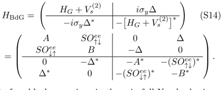
the Bogoliubov-de Gennes form

H

BdG

= H

_G

+ V

s⁽²⁾

iσ

_y

∆

−iσ

y

∆

^∗

−

H

G

+ V

s⁽²⁾

^∗

!

(S14)

=







A SO

^ee_↑↓

0 ∆

SO

^ee_↓↑

B −∆ 0

0 −∆

^∗

−A

^∗

−(SO

_↑↓^ee

)

^∗

∆

^∗

0 −(SO

^ee_↓↑

)

^∗

−B

^∗





 .

Its four blocks are given in the spin-full Nambu basis Ψ =

Ψ

_↑^e

, Ψ

_↓^e

, Ψ

_↑^h

, Ψ

_↓^h

^>

, (S15)

where Ψ

^e_σ

(Ψ

^h_σ

) stands, schematically, for an array of all annihilation (creation) operators with spin σ that operate on local atomic orbitals residing on the real-space lattice (graphene + adatom). Components A, B, SO

_↑↓^ee

, and SO

^ee_↓↑

represent spin-conserving and spin-flipping tight- binding matrix elements in the normal phase. Each of them is a matrix, whose entries are labeled by the two lattice sites’ indices. For example, the element A

_m,n

rep- resents spin-conserving hopping of an electron with spin up from the site n to site m. Since we are interested in the spin relaxation of QPs, a more convenient implementa- tion in Kwant relies on the global unitary transformation

U =







1 0 0 0 0 0 0 1 0 0 1 0 0 1 0 0







, (S16)

which transforms the Hamiltonian H

_BdG

into

H

_BdG⁰

=







A ∆ 0 SO

_↑↓^ee

∆

^∗

−B

^∗

−(SO

_↓↑^ee

)

^∗

0 0 −(SO

_↑↓^ee

)

^∗

−A

^∗

−∆

^∗

SO

_↓↑^ee

0 −∆ B





 .

(S17) This representation is tailored to the basis (γ

_↑

, γ

_↓

)

^>

, con- sisting of two reduced particle-hole Nambu spinors

γ

↑

=

Ψ

_↑^e

, Ψ

_↓^h

>

and γ

↓

=

Ψ

_↑^h

, Ψ

_↓^e

>

. (S18) The above transformation eventually partitions the Hamiltonian into two blocks—the up-spin QP sec- tor γ

↑

(upper-left corner) and the down-spin QP sec- tor γ

↓

(lower-right corner). Those blocks are cou- pled by the off-diagonal spin-flip perturbation Hamilto- nian (sparse matrix) that encompasses just the spin-flip part of the local SOC (or magnetic exchange). The total Hamiltonian takes therefore the form

H

_BdG⁰

=

H

γ↑γ↑

H

_γ^SO_↑_γ_↓

H

_γ^SO_↓_γ_↑

H

_γ_↓_γ_↓

. (S19)

Making use of H

_BdG⁰

significantly simplifies not only

the implementation of the QP scattering problem

(5)

V in Kwant [see also Fig. S2 and the detailed description in

its caption], but also the interpretation of the obtained results in terms of the S-matrix entries. The reduced Nambu basis naturally separates the QP spins, and, more importantly, allows us to directly compute the supercon- ducting S-matrix, which is not so obvious in the original basis due to Kwant code specific technicalities (“conser- vation laws”).

In order to effectively simulate 2D bulk transport em- ploying the 1D ribbon calculation, we follow the method presented, for example, in Ref. [S14]. Particularly, we im- pose Φ-periodic boundary conditions (PBCs) along the transverse y-direction that promote hoppings between the sites (x, y = 0) and (x, y = W ) lying on opposite edges of the 1D ribbon (W stands for its width). Those hoppings enter H

γ↑γ↑

and H

γ↓γ↓

terms in Eq. (S19). For the sake of brevity, we represent them in the tight-binding form using γ

↑

and γ

↓

operators at sites (x, 0) and (x, W ):

hop

^Φ-PBC

= γ

_↑,(x,W)^†

−te

^−iΦ

0 0 te

^−iΦ

γ

_↑,(x,0)

+ γ

_↓,(x,W)^†

te

^+iΦ

0 0 −te

^+iΦ

γ

_↓,(x,0)

+ h.c., (S20) where the angle Φ ∈ [0, 2π], and t is the nearest neigh- bor graphene hopping. Note that the phase factors in the γ

_↓

-part should be complex conjugated in order to preserve time-reversal symmetry of the unperturbed su- perconducting host. This additional phase factors allow for accessing different transverse momenta k

y

and thus for the simulation of 2D transport characteristics. A de- tailed scheme how that works is illustrated in Fig. S3 for ordinary graphene. Finite width of the scattering re- gion discretizes the allowed values of the transverse mo- menta k

y

and the resulting 1D band structure foliates into several projected subbands. Changing Φ in the PBCs, the originally discrete k

_y

levels in k-space shift by an equal amount and different sets of 2D graphene states can therefore be addressed. Averaging over many dif- ferent phases basically leads to a reliable sampling of 2D graphene’s Brillouin zone and hence to bulk trans- port simulations which can be well compared with an- alytical results. The aforementioned strategy and im- plementation is used to numerically obtain the S-matrix elements.

To treat the magnetic moment-mediated spin relax- ation of QPs, we proceed in exactly the same way, i.e., we start from the Hamiltonian H

BdG

, Eq. (S14), but we use the effective Hamiltonian ˜ V

s⁽¹⁾

, Eq. (S10), instead of V

s⁽²⁾

, and then follow the same steps as in the above SOC case.

Spin relaxation rates from Kwant

Knowing the S-matrix entries as functions of chem- ical potential, the QP energy, and the incoming and

outgoing modes, we can compute the QP spin-flip rate 1/τ

s

(E) at energy E, and consequently the total spin-flip rate 1/τ

s

(µ, T ) in the superconducting phase held at chemical potential µ and temperature T. The fermionic nature of QP excitations implies that those two rates are related [S2, S16] via the formula

1 τ

_s

(µ, T ) =

∞

R

∆

dE QP-DOS

_sr

(E)

−

_∂E^∂g

1 τs(E)

∞

R

∆

dE QP-DOS

_sr

(E)

−

_∂E^∂g

, (S21) where the integration is taken over all QP energies, QP-DOS

_sr

(E) represents the unperturbed QP density of states in the scattering region at energy E, and g(E, T ) = [exp (E/k

_B

T) + 1]

⁻¹

is the Fermi-Dirac dis- tribution [note that QP energies are measured relative to µ since the latter explicitly enters the model Hamil- tonian H

_g

]. In what follows, we derive the expressions for 1/τ

_s

(E) and QP-DOS

_sr

(E) employing solely the en- tries accessible from the Kwant package, and then, using Eq. (S21), we compare the numerical approach with our analytical calculations.

Kwant provides S-matrix entries among different leads’

modes that are labeled by spin σ, energy E, and a set {n}

of other discrete indices. For example, in our 1D problem the latter represent the transverse lead mode quantum number and the direction of motion—encoded in the su- perscripts L and R [convention used in Fig. S2: incoming (outgoing) L-/R-mode departs from (arrives at) L-/R- lead]. In sequel, we suppress most of them and, for the sake of brevity, we use just collective labels i and o for the incoming and outgoing modes, and the spin index σ = {↑, ↓}. Our system, displayed in Fig. S2, consists of spin-up and spin-down QP semi-infinite leads with width W , and a scattering region with length L and width W that hosts 4W L/( √

3a

²

) carbon atoms [graphene lattice constant a = 2.46 ˚ A] and one impurity, hence concentra- tion

η =

√ 3a

²

4W L . (S22)

Assuming that there is an incoming QP mode (i, σ) at energy E, the probability p

−σ,σ

(i, E) measuring that the mode (i, σ) experiences a spin-flip equals

p

_−σ,σ

(i, E) = X

o

S

_−σ,σ^o,i

(E)

2

, (S23)

where the sum over o runs over all outgoing modes (o, −σ) at energy E. Then, the average QP spin- flip probability at energy E reads

p

_s

(E) = 1 2#

i

X

i

p

_↑,↓

(i, E) + 1 2#

i

X

i

p

_↓,↑

(i, E), (S24)

where the term in the denominator #

i

counts the number

of accessible incoming modes per spin at energy E. The

(6)

VI factor 1/2 takes into account the probability—picking a

QP at energy E, it is equally likely to have up- or down- spin.

It is specific to the Kwant package to associate with each incoming mode (i, σ) the lead wave function |Ψ

i,σ

i, such that its scalar product over the lead-unit cell [that covers spatial area a × W and the number of 2W/( √

3a) of graphene unit cells along the transverse direction] is given as follows

hΨ

i,σ

|Ψ

i,σ

i

luc

= 1

~ a

v

g

(i) , (S25) where v

g

(i) stands for the magnitude of group velocity of the mode (i, σ). Since the underlying system is not magnetic, the corresponding QP energies and group ve- locities are same for both spin projections. The Kwant normalization of |Ψ

_i,σ

i implies that the QP DOS in the lead unit cell equals

QP-DOS

_luc

(E) = 1 2π

X

(i,σ)

hΨ

_i,σ

|Ψ

_i,σ

i

_luc

, (S26)

and, therefore, the unperturbed QP DOS in the scatter- ing region L × W is given as follows

QP-DOS

_sr

(E) = L

a

QP DOS

_luc

(E). (S27) The average time t(E), the incoming QP at energy E would need in order to scatter into a family of empty outgoing modes would be the average of L/v

_g

(i) over all incoming modes, i.e.,

t(E) = 1 2#

i

X

(i,σ)

L

v

g

(i) = L/a 2#

i

X

(i,σ)

a

v

g

(i) (S28)

= ~ L/a 2#

i

X

(i,σ)

hΨ

i,σ

|Ψ

i,σ

i

luc

= 2π ~ 2#

i

QP-DOS

_sr

(E),

where we have used Eqs. (S25)-(S27). Dividing the aver- age spin-flip probability p

s

(E) by the average time t(E) gives the average QP spin-flip rate at energy E,

1 τ

_s

(E) = 1 2π ~

P

i,o

S

_↑,↓^o,i

(E)

2

+

S

_↓,↑^o,i

(E)

2

QP-DOS

_sr

(E) . (S29) Plugging the partial results, Eqs. (S26) (S27) and (S29), into the main formula for the spin-relaxation rate 1/τ

s

(µ, T ), Eq. (S21), we get the central result of this section—the Kochan-Barth formula © :

1 τ

_s^Kw

=

a L

~

∞

R

∆

dE

−

_∂E^∂g

P

i,o,σ

S

_−σ,σ^o,i

(E)

2

∞

R

∆

dE

−

_∂E^∂g

P

(i,σ)

hΨ

i,σ

|Ψ

i,σ

i

luc

. (S30)

The quantities on the right-hand side, the entries of S- matrix, and the lead wave functions are fully accessible from the Kwant calculation. Multiplying the nomina- tor of the above fraction by unity, written in the form (4W )/( √

3a) × ( √

3a)/(4W ), we can write

1 τ

_s^Kw

=

η

^√^4W

3a

~

∞

R

∆

dE

−

_∂E^∂g

P

i,o,σ

S

_−σ,σ^o,i

(E)

2

∞

R

∆

dE P

(i,σ)

hΨ

i,σ

|Ψ

i,σ

i

luc

−

_∂E^∂g

. (S31)

The energy integration is numerically evaluated employ- ing the Riemann summation, where we integrate from the band gap ∆ to a energy cut-off of ∆ + 25k

B

T . In or- der to have a higher resolution close to the band gap ∆, we split the integral into two integration regions. First, we integrate from ∆ to ∆ + 3.5k

_B

T with 15 steps and second, to ∆ + 25k

_B

T with 25 steps. We keep the same partitioning prescription for all temperatures keeping the same number of points within the corresponding regions, so that all integrated results have the same “systematic error”. To keep a reasonable balance between the com- putational efforts and the required accuracy, we restrict our calculations to a scattering region of length L = 5 a and width W = 299 a (we checked that without includ- ing a disorder the dependence on L is substantially less pronounced than that on W , there we use such elon- gated geometry). For averaging over the angle that enters Φ-PBC, we choose 20 equally distributed values within [0, 2π]. Given our parameters, the correspond- ing η

_Kwant

equals 288 ppm.

The results of the Kwant package calculations are presented in Figs. S4 and S5, respectively, along with the corresponding data from the analytic T-matrix ap- proach presented in the opening subsection to that para- graph. Similarly as in the main text, Fig. S4 displays the magnetic-impurity-scenarios and Fig. S5 the SOC- dominated regimes, each for hydrogen [panels (a)] and fluorine [panels (b)]. Comparing the Kwant -computed results with the analytical ones, as also presented in the main text [see Figs. 2(a) and (b), as well as Fig. 3 therein], we see the striking qualitative and quantita- tive agreements between both approaches over the whole ranges of doping and temperature. All distinguished characteristics as observed analytically occur simulta- neously in the numerical Kwant simulations, serving as an unprecedented evidence of our predictions’ self- consistency. Therefore, we believe that our findings are universal and potentially interesting for spin-relaxation experiments that can, then, resolve the dominant spin- relaxation mechanism in graphene.

As a comment, the numerically determined spin-

relaxation curves are not as smooth as the analytical

ones since we need to restrict ourselves to reasonable

scattering region sizes; otherwise, the computational ef-

forts would become unmanageable and too expensive.

(7)

VII

k

y

[nm

¹

]

3 2 1 0 1 2 3 _{3 2 1}

k

^{0 1 2}^x

[nm

³¹

]

E [eV]

3 2 1 0 1 2 3

k

y

[nm

¹

]

3 2 1 0 1 2 3 4 _{3 2 1}

k

^{0 1 2}^x

[nm

³¹

]

E [eV]

3 2 1 0 1 2 3

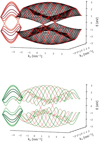
FIG. S3. The phase-averaging scheme with Φ-periodic bound- ary conditions for graphene in the normal phase. Top: Elec- tronic band structure of 2D graphene (3D black mash) versus momenta (k

x

, k

y

). The finite width of the sample along the y-direction quantizes the allowed values of k

y

what is giving the discretized electronic dispersion (red lines on top of the 3D black mesh). Projecting the latter along k

y

in the Bril- louin zone gives the distinct k

x

-dependent projected subbands shown on the left (displayed in different tones of red). Bot- tom: Changing the phase of exp(±iΦ) in the PBCs shifts the discretized electronic dispersion—schematically, the original red bands move to the green ones. The resulting subbands give rise to the new projected band structure (displayed on the left in different tones of green). Sampling Φ ∈ [0, 2π] cov- ers different incoming and outgoing modes by allowing dif- ferent transverse momenta k

y

. This enables us to simulate 2D bulk transport characteristics within a 1D ribbon geome- try.

The limited size of the scattering region and the afore- mentioned phase averaging over the transverse modes raise some numerical fluctuations, which—although be- ing clearly evident—do not spoil the qualitative behav- ior. Moreover, finite-size effects cause that the value of η needed to align analytical calculations (in most cases

280 ppm) with the numerical results slightly deviates from the corresponding η

Kwant

(288 ppm). The finite size effects are mostly visible in the case of SOC in hy- drogenated graphene, Fig. S5(a). This is because the typical energy separation due to finite width W is about 5 meV while the dominant SOC scale Λ

^B_PIA

' 1 meV, in that case to match numeric with analytic we need efec- tively lower η = 220 ppm.

(ANTI -)HEBEL-SLICHTER EFFECT IN RESONANT MAGNETIC

JOSEPHSON JUNCTIONS

In the main text, we attributed the breakdown of the Hebel-Slichter effect in superconducting graphene to a substantial energy separation between the QP excitations that reside at the coherence peaks and YSR bound states around impurities whose energies immerse deep in- side the superconducting gap. It is well known (see, for example Ref. [S17] and references therein) that such YSR states determine underlying spectral and spin char- acteristics. For instance, they are responsible for 0- π transitions in magnetic Josephson junctions that re- verse the direction of the supercurrent. This section demonstrates yet on another example—resonant mag- netic Josephson junctions—that the observed breakdown of the Hebel-Slichter effect seems to be a universal phys- ical phenomenon that accompanies QP spin transport through magnetic resonances in s-wave superconductors.

We consider the one-dimensional Josephson geome- try depicted in Fig. S6(a). Two semi-infinite super- conductors are coupled via the “resonant superconduct- ing trap” with width a (not related to the graphene lat- tice constant). The latter is composed of two outer ul- trathin deltalike scalar tunnel barriers—residing at z = 0 and z = a, respectively—and the additional host—

deltalike magnetic impurities—intercalated in the mid- dle, i.e., at z = a/2. Such a configuration enables a full analytical treatment, yielding a relatively simple and vi- sual toy model of resonant magnetic impurity scattering inside Josephson junctions that allows to qualitatively and quantitatively explore its spin-flip properties.

Scattering of QPs and the formation of YSR states in the above resonant setup can be described in terms of the Bogoliubov-de Gennes Hamiltonian [S16] that needs to be formulated within the spin-full Nambu basis,

H

BdG

=

H

_e

∆(z)

∆

^†

(z) H

h

. (S32)

It couples the single electronlike QP Hamiltonian H

e

=

− ~

²

2m

d

²

dz

²

− µ

σ

0

+ λ

SC

σ

0

δ(z) + δ(z − a) +

λ

MA,z

σ

z

+ λ

MA,x

σ

x

δ(z − a/2) (S33)

(8)

VIII

FIG. S4. Comparison of Kwant (symbols) and analytical (solid lines) calculations of QP spin-relaxation rates in superconducting graphene in the presence of hydrogen [panel (a)] and fluorine [panel (b)] magnetic impurities with concentration (per carbon atom) η

Kwant

= 288 ppm. Both methods match and provide consistent qualitative and quantitative pictures regarding the temperature and doping dependencies of 1/τ

s

, and its enhancement and depletion depending on the position of the Fermi level µ with respect to resonances. Rainbow arrows indicate the expected increase of the spin relaxation with lowered temperature outside the resonances—the Hebel-Slichter effect—and its predicted break-down [substantial decrease of the spin-relaxation] near the resonances due to emergent YRS states deep inside the superconducting gap. Magnetic exchange coupling is J = −0.4 eV for hydrogen, and J = 0.5 eV for fluorine, the Kwant simulation used a scattering region with W = 299 a and L = 5 a. Analytical results require slightly lower concentrations η [values are inside the plots] to be perfectly aligned with the Kwant data. The reasons for that are originating from finite-size effects and the finite number of phases used in the PBC averaging.

FIG. S5. Comparison of Kwant (symbols) and analytical (solid lines) calculations of QP spin-relaxation rates in superconducting graphene in the presence of locally enhanced SOC for hydrogen [panel (a)] and fluorine [panel (b)] impurities with η

Kwant

= 288 ppm. Both methods match perfectly and provide the same qualitative and quantitative features regarding the temperature and doping dependencies of 1/τ

s

. Rainbow arrows evolving from red to blue indicate the expected decreasing trend of the spin relaxation with lowered temperature. SOC parameters are given in Table S1 and the geometrical setup is the same as in Fig. S4. Analytical results require slightly lower concentrations η [values are inside the plots] to be perfectly aligned with the Kwant data [W = 299 a and L = 5 a]. The reasons for that are originating from finite-size effects and the finite number of phases used in the PBC averaging.

with its holelike counterpart H

_h

= −σ

y

H

_e^∗

σ

_y

, en- wrought through the s-wave superconducting pairing po- tential ∆(z) = ∆ σ

₀

. We assume the outer (semi-infinite) superconductors possess the same superconducting en- ergy gap ∆ and that the junction is not subject to any superconducting phase difference. To further sim-

plify the analytical treatment, we consider also equal QP masses m and chemical potentials µ. The scat- tering strengths of the two identical outer barriers are parameterized by the scalar λ

_SC

, whereas the magnetic scattering strengths in the middle are governed by λ

MA,z

and λ

MA,x

, accordingly. The latter acts perpendicular

(9)

IX

resonant trap

scalar magnetic SCATTERING

scalar

0 -1 -0.5 0 0.5 1

-4 -3 -2 -1 0 1 2 3 4

E

YSR

/ ∆

Magnetic scattering strength (a)

(b)

FIG. S6. (a) Schematic sketch of the one-dimensional res- onant magnetic Josephson junction (oriented along ˆ z), cou- pling two semi-infinite superconducting electrodes (light red) via the resonant superconducting trap (light blue) with width a. The latter consists of two outer deltalike tun- neling barriers at z = 0 and z = a, parameterized by scalar strength λ

SC

, and the central deltalike barrier at z = a/2 mimicking magnetic impurity scattering, pa- rameterized by λ

MA,z

and λ

MA,x

, respectively. An In- cident QP with spin σ—IN

^σ

—arrives from the left su- perconductor and can be reflected back as a QP with spin σ

⁰

—probability R

^σ,σ⁰

—or transmitted through the reso- nant trap—probability T

^σ,σ⁰

. (b) Calculated energies of the YSR bound states, E

YSR

, normalized to the magnitude ∆ of the superconducting gap, as a function of the (dimension- less) magnetic strength λ

MA,z

= (2mλ

MA,z

)/( ~

²

q

F

). We as- sume fixed scalar and magnetic λ

MA,x

scattering strengths such that λ

SC

= (2mλ

SC

)/( ~

²

q

F

) = 2 and λ

MA,x

= (2mλ

MA,x

)/( ~

²

q

F

) = 1, as well the representative chemi- cal potential µ = 200 meV = 200∆

0

∆

0

. The width of the resonant trap is a = 10 nm. The magnetic impurity strength controls a wide parameter region in which the YSR states are immersed deep inside the superconducting gap (emphasized by shading).

to the QPs initial spin quantization axis (ˆ z) and induces thus spin-flip scattering. As usual, σ

0

denotes the two- by-two identity matrix and σ

i

the ith Pauli matrix, all acting in spin space.

To unravel the energies of the YSR states that form around the central magnetic barrier of the junction, we

follow the same strategy as described in Ref. [S17]. Re- garding the model parameters, we use the same supercon- ducting gap and the critical temperature as for supercon- ducting graphene, i.e., ∆

₀

= 1 meV and T

_c

' 6.593 K.

Furthermore, we take a representative chemical poten- tial, µ = 200 meV = 200∆

₀

∆

₀

, with the corre- sponding Fermi wave vector q

_F

= √

2mµ/ ~ . For the scalar and magnetic λ

_MA,x

scattering strengths, we im- pose the moderate values λ

SC

= (2mλ

SC

)/( ~

²

q

F

) = 2 and λ

MA,x

= (2mλ

MA,x

)/( ~

²

q

F

) = 1—as motivated by [S18]—, while the resonant trap’s width is set to a = 10 nm. Figure S6(b) displays the computed energies of the subgap states as a function of the magnetic scat- tering strength λ

MA,z

= (2mλ

MA,z

)/( ~

²

q

F

), confirm- ing the previously observed behavior [S17]. As long as λ

MA,z

inside the trap is smaller than |λ

MA,z

| . 0.04, the bound state spectrum contains only the usual An- dreev states at E

ABS

= ±∆ and lacks the YSR counter- parts. Contrary, going over that value, |λ

MA,z

| & 0.04, the spectrum starts to host also YSR states. Their ener- gies are deeply immersed inside the gap so that one can expect reduced spin-flip scattering. Magnetic Joseph- son junctions’ spectral properties are effectively tuned by changing λ

MA,z

, which serves as the control param- eter for tuning the energies of the YSR states in this section. Contrary to the case of graphene, where that was done by varying the chemical potential.

In the main text, we argued that magnetic impurities are expected to significantly impact the QP spin-flip scat- tering characteristics in resonances, and thereby cause the breakdown of the Hebel-Slichter effect. That this is not a red herring inherent to the nature of superconduct- ing graphene is demonstrated now by the 1D resonant magnetic Josephson junction with |λ

MA,z

| & 0.04, sup- porting deeply immersed YRS states. Instead of com- puting the QP spin-relaxation rate 1/τ

_s

, which can be measured directly in experiments, we compute a from the theoretical viewpoint equivalent physical quantity, namely the QP spin-flip scattering probability P

spin-flip

. The latter is given by

P

spin-flip

= X

σ

X

σ⁰=−σ

1 2

× R

E⁰

∆

dE

R

^σ,σ⁰

(E) + T

^σ,σ⁰

(E)

QP DOS(E)

−

_∂E^∂g

R

E⁰

∆

dE QP DOS(E)

−

_∂E^∂g

,

(S34)

counting the same spin-flip scattering processes that

would determine the spin-relaxation rate, averaged over

all excited QP states starting from the ground state en-

ergy ∆. Regarding the computational details, we con-

sider an incoming QP with spin σ that enters from

the left superconducting electrode and can either be re-

flected back or transmitted through the resonant mag-

netic trap into the right superconductor as a QP with

(10)

X

0 1 2 3 4 5

-0.4 -0.3 -0.2 -0.1 0 0.1 0.2 0.3 0.4

Magnetic scattering strength

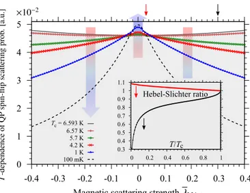
T_c= 6.593 K 6.57 K 5.7 K 4.2 K 1 K 100 mK

0.3 0.4 0.5 0.6 0.7 0.8 0.9 1 1.1

0 0.2 0.4 0.6 0.8 1

Hebel-Slichter ratio

T/Tc

FIG. S7. QP spin-flip scattering probability at different tem- peratures and as a function of λ

MA,z

; the remaining param- eters are the same as in Fig. S6(b). With decreasing tem- perature, the spin-flip scattering probabilities increase in the region where the YSR states overlap with the edges of the superconducting gap and decrease in the regions where the YSR states move into the gap. The shaded region shows the related normal-phase spin-flip probability (as a guide for eyes). Rainbow arrows (coded in colors of temperature descent) indicate the raising (upward arrow) and lowering (downward arrow) trends of the spin-flip scattering prob- ability as temperature goes down, starting at T

c

(normal phase). The inset shows the corresponding Hebel-Slichter ra- tio, P

spin-flip

(T )/P

spin-flip

(T

c

), as a function of T /T

c

and at two representative magnetic scattering strengths (indicated by red and black arrow ticks on the top horizontal axis):

λ

MA,z

= 0.03 (see red circled data) and λ

MA,z

= 0.3 (see black circled data).

spin σ

⁰

= −σ. The scattering probabilities for the re- flection and transmission of the incident QP with en- ergy E are denoted by R

^σ,σ⁰

(E) and T

^σ,σ⁰

(E), respec- tively. They are computed in the standard way as ab- solute squares of the amplitudes that come from the standard wave-function matching at each delta barrier.

Recall that the QP DOS is given by QP DOS(E) =

√ E

E²−∆²

DOS(µ) and the temperature dependence of the superconducting gap scales according to the BCS the- ory [S16], i.e., ∆ = ∆

0

tanh(1.74 p

T

c

/T − 1). The up- per limits in the above integrals should be infinities, but because of the thermal smearing (−

_∂E^∂g

), the dominant contributions come from those QP states that reside in the coherence peaks. It is therefore most important to cover primarily that energy range, recognizing that the coherence peaks’ energy widths scale ∼ ∆. Since the chemical potential µ is set to a large value anyway, we take E

⁰

= p

µ

²

+ ∆

²

∆ as the upper integration limits in the above formula for P

_spin-flip

.

Figure S7 presents the calculated QP spin-flip scat- tering probabilities as functions of temperature and the

magnetic scattering strength λ

MA,z

. We decrease the overall temperature in the same way as for superconduct- ing graphene, see Figs. 2 and 3 in the main text. The range of λ

_MA,z

is rather narrow to cover the crossover from the usual Hebel-Slichter scenario to its resonant breakdown. Comparing the outcomes with the YSR en- ergies in Fig. S6(b), we observe the same trends as ini- tially predicted for superconducting graphene. Hence, we can state the following conclusions: (1) superconducting systems hosting magnetic impurities support the usual Hebel-Slichter effect only when the YSR states overlap or are very close to the QP coherence peaks (for the considered junction, |λ

MA,z

| . 0.04). In these cases, the related QP spin-flip scattering probabilities increase with decreasing temperature. Contrary to that, (2) once the strength of λ

MA,z

(or another control parame- ter) starts to immerse the energies of YSR state deep in- side the superconducting gap (for the considered junction,

|λ

MA,z

| & 0.04), the Hebel-Slichter effect breaks down and

lowered temperature depletes the QP spin-flip processes.

Our findings serve as yet further evidence that sup- ports the physical explanation of the Hebel-Slichter ef- fect’s breakdown at magnetic resonances and gives our findings more universal validity not limited just to graphene. Investigating the temperature dependence of QP spin relaxation in superconducting systems might provide a novel experimental tool to unravel the dom- inant spin-relaxation mechanisms and simultaneously sheds new light on the physics of YSR states.

[S1] J. R. Schrieffer, Theory of Superconductivity (Benjamin, New York, 1964).

[S2] Y. Yafet, Physics Letters A 98, 287 (1983).

[S3] L. C. Hebel and C. P. Slichter, Physical Review 107, 901 (1957).

[S4] L. C. Hebel and C. P. Slichter, Physical Review 113, 1504 (1959).

[S5] L. C. Hebel, Physical Review 116, 79 (1959).

[S6] D. Kochan, S. Irmer, and J. Fabian, Physical Review B 95, 165415 (2017).

[S7] M. Gmitra, D. Kochan, and J. Fabian, Physical Review Letters 110, 246602 (2013).

[S8] S. Irmer, T. Frank, S. Putz, M. Gmitra, D. Kochan, and J. Fabian, Physical Review B 91, 115141 (2015).

[S9] M. Gmitra, S. Konschuh, C. Ertler, C. Ambrosch-Draxl, and J. Fabian, Phys. Rev. B 80, 235431 (2009).

[S10] I. ˇ Zuti´ c, J. Fabian, and S. Das Sarma, Reviews of Mod- ern Physics 76, 323 (2004).

[S11] J. Fabian and M. W. Wu, in Handbook of Spin Trans- port and Magnetism, edited by E. Tsymbal and I. ˇ Zuti´ c (CRC Press, Taylor & Francis Group, 2012) pp. 303–

327. [S12] D. Kochan, M. Gmitra, and J. Fabian, in Symmetry,

Spin Dynamics and the Properties of Nanostructures,

Lecture Notes of the 11th International School on The-

oretical Physics, edited by J. Barna´ s, V. Dugaev, and

(11)