Virtual Reality & Physically-Based Simulation

(1)

Virtual Reality &

Physically-Based Simulation

Sound Rendering

G. Zachmann

University of Bremen, Germany

cgvr.cs.uni-bremen.de

(2)

G. Zachmann Virtual Reality WS 18 December 2013 Sound Rendering 2

C C

Sound in VR

§  Reminder: complete immersion = all human senses are being stimulated consistently

§  (Counter-example: watch a thriller on TV without sound! J)

§  Some of the functions of our auditory sense:

§  Localization of not (yet) visible sound sources (e.g., predator)

§  Our second most important sense for navigation (e.g., in buildings)

§  Allows us to obtain a sense of the space around us

§  Auditory impressions (Höreindrücke):

§  "Big" (late reverberations),

§  "cavernous" (lots of echos),

§  "mufﬂed" (no reverberations),

§  "outside" (no echos, buts many other sounds).

§  How to render sound: in the following, only "sound propagation" (no sound synthesis)

(3)

C C

Digression: the Cocktail Party Effect

§ 

Describes the ability of humans to extract a single sound source from a complex

auditory environment (e.g., cocktail party)

§ 

Challenges:

§  Sound segregation

§  Directing attention to sound source of interest

Breakfast at Tiffany’s (Paramount Pictures)

Current Biology Vol 19 No 22 R1026

locations in a room. As some sources are closer to a microphone than others, each microphone yields a different weighted combination of the sources. If there are as many microphones as there are sources, rudimentary assumptions about the statistical properties of sources (typically, that they are non-Gaussian according to some criterion) often

suffice to derive the source signals from the mixtures.

Biological organisms, however, have but two microphones (our ears), and routinely must segregate sounds of interest from scenes with more than two sources. Moreover, although sound segregation is aided by binaural localization cues, we are not dependent on them — humans

generally can separate sources from a monaural mixture. Indeed, much popular music of the 20^th century was recorded in mono, and listeners can nonetheless hear different instruments and vocalists in such recordings without trouble. The target speech of Figure 2 is also readily understood from monaural mixtures of multiple talkers. It is thus clear that biological auditory systems are doing something rather different from standard ICA algorithms, though it remains possible that some of the principles of ICA contribute to biological hearing. At present we lack effective engineering solutions to the ‘single microphone’

source separation problem that biological auditory systems typically solve with success.

Auditory versus visual segmentation Segmentation is also a fundamental problem for the visual system. Visual scenes, like auditory scenes, usually contain multiple objects, often

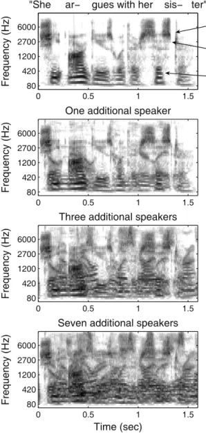
scattered over complex backgrounds, and the visual system must recognize individual objects amid this clutter (Figure 1). However, several salient differences between visual and auditory scenes make the auditory segmentation problem particularly difficult. The first is that visual objects tend to occupy local regions on the retina. Sound sources are, by comparison, spread out across the frequency map of the cochlea (as is apparent in Figure 2). As a result, their sensory representation often overlaps considerably more than do those of visual objects. A second difference compounds this problem — sound sources add linearly to create the signal entering the ears, whereas visual objects occlude each other. If objects are opaque, as they usually are, the object nearest the viewer determines the image content at its location. The sound energy at a particular time and frequency, by contrast, is a sum across every sound source in the auditory scene. The upshot is that the more people there are at a party, the harder it will be to hear the person standing next to you, as the sounds made by each additional person will at various points in time mask the speaker of interest. The speaker’s face, in contrast, will remain perfectly visible unless someone steps in front of them (Figure 1).

The situation with sound is perhaps most analogous to what the visual

Frequency (Hz)

"She ar− gues with her sis− ter"

0 0.5 1 1.5

6000 2700 1200 420 80

0 0.5 1 1.5

6000 2700 1200 420 80

0 0.5 1 1.5

6000 2700 1200 420 80

0 0.5 1 1.5

6000 2700 1200 420 80

0 0.5 1 1.5

6000 2700 1200 420 80

0 0.5 1 1.5

6000 2700 1200 420 80

0 0.5 1 1.5

6000 2700 1200 420 80

Frequency (Hz)

One additional speaker

Frequency (Hz)

Three additional speakers

Frequency (Hz)

Seven additional speakers

Time (sec) Time (sec)

−50

−40

−30

−20

−10 0 Common onset

Common offset

Harmonic frequencies Level (dB)

Current Biology

Figure 2. Cocktail party acoustics.

Spectrograms of a single ‘target’ utterance (top row), and the same utterance mixed with one, three and seven additional speech signals from different speakers. The mixtures ap- proximate the signal that would enter the ear if the additional speakers were talking as loud as the target speaker, but were standing twice as far away from the listener (as might occur in cocktail party conditions). Spectrograms were computed from a filter bank with bandwidths and frequency spacing similar to those in the ear. Each spectrogram pixel represents the rms amplitude of the signal within a frequency band and time window. The spectrogram thus omits local phase information, which listeners are insensitive to in most cases. The gray- scale denotes attenuation (in dB) from the maximum amplitude of all the pixels in all of the spectrograms, such that gray levels can be compared across spectrograms. Acoustic cues believed to contribute to sound segregation are indicated in the spectrogram of the target speech (top row). Spectrograms in the right column are identical to those on the left except for the superimposed color masks. Pixels labeled green are those where the original target speech signal is more than –50 dB but the mixture level is at least 5 dB higher. Pixels labeled red are those where the target was less and the mixture was more than –50 dB in amplitude.

The sound signals used to generate the spectrograms can be listened to at http://www.cns.

nyu.edu/~jhm/cocktail_examples/.

(4)

C C

Naïve Methods

§  Sound in games, e.g., noise from motors or guns

§  Sound = function of speed, kind of car/gun, centrifugal force, orientation of plane, etc.

§  Sounds have been sampled in advance

§  Simple "3D" sound:

§  Compute difference in volume of sound that reaches both ears

§  Possibly add some reverberation (Nachhall)

§  But how to render sound realistically and in real-time?

§  Differences between light and sound:

§  Velocity of propagation (sound = 343 m/s in air)

§  Wavelength

Ø Makes rendering of sound so difﬁcult

Sound source

Listener

(5)

C C

Human Factors

§  Akustische Effekte:

§  Reﬂexion (reﬂection),

§  Brechung (refraction),

§  Streuung,

§  Beugung (diffraction),

§  Interferenz.

§  Ortungsfähigkeit des Ohrs:

§  Amplitudendifferenz,

§  Laufzeitunterschiede,

§  Änderungen des Spektrums durch Ohrmuschel und Kopf.

from Isaac Newton's Principia (1686)

(6)

C G C C G C

Version for review

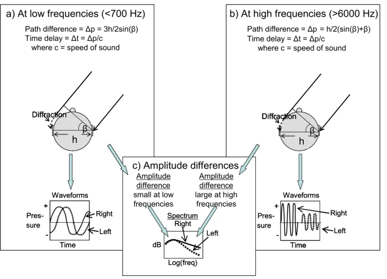
Figure 1. Inter-aural differences for a plane wave arriving at azimuth radians.

Panel a): At low frequencies, when the wavelength of sound is large compared with the width (h) of the head, the inter-aural difference is mainly one of time of arrival, and is less than the duration of a single cycle.

Panel b): At high frequencies, when the wavelength of sound is small compared with the width of the head, less energy travels to the far ear by diffraction. As a result, there are inter-aural differences of both amplitude and time J and the latter can amount to the duration of several cycles.

Panel c): The frequency-dependence of amplitude differences results in a spectral difference.

h

Diffraction

a) At low frequencies (<700 Hz)

Path difference = p = 3h/2sin( ) Time delay = t = p/c

where c = speed of sound

Time +

Pres- -

Right Left +

sure - +

-

Waveforms

h

Diffraction

b) At high frequencies (>6000 Hz)

Path difference = p = h/2(sin( )+ ) Time delay = t = p/c

Time +

-

Right Left Time

+

-

Waveforms +

- +

- Pres- sure

c) Amplitude differences

Amplitude difference small at low frequencies

Amplitude difference large at high

frequencies

Log(freq) dB

Right

Left Spectrum

h

Diffraction

Time +

Pres- -

Right Left +

sure - +

-

Waveforms

h

Diffraction

h

Diffraction Diffraction

Time +

Pres- -

Right Left +

sure - +

-

Waveforms

Time +

Pres- -

Right Left +

sure - +

-

Waveforms

h

Diffraction

Time +

-

Right Left Time

+

-

Waveforms +

- +

- Pres- sure

h

Diffraction

h

Diffraction Diffraction

Time +

-

Right Left Time

+

-

Waveforms +

- +

- Pres- sure

Time +

-

Right Left Time

+

-

Waveforms +

- +

- Pres- sure

frequencies

Log(freq) dB

Right

Left Spectrum

frequencies

Log(freq) dB

Right

Left Spectrum

Log(freq) dB

Right

Left Spectrum

Wellenlänge groß relativ zur Kopfgröße → starke Beugung um Kopf →

nur Zeitverschiebung zwischen den Ohren

Wellenlänge klein relativ zur Kopfgröße → schwache Beugung um Kopf →

Zeitverschiebung und Lautstärkedifferenz zwischen den Ohren

(7)

C C

Mischen von Schallquellen

§  

n Quellen aus verschiedenen Richtungen, jede sendet ein Signal s_i(t)

§  

Dämpfung ("attenuation") a_i pro Quelle s_i:

§ 

Summe:

Listener

Source

Source Source

Source

l_i

s_i

a

_i

= e

_i

(

_i

, ⇥

_i

)e

_r

(

_i

, ⇥

_i

)v

_i

l

_i

e

_i

( , ⇥) = Abstrahlchar. z.B.

¹₂

(1 + cos( )

^↵

) e

_r

= Empf¨angerchar.

v

_i

= visibility, incl. Beugung, 2 [0, 1]

l

_i

= Entfernung

s (t ) = X

i

a

_i

s

_i

(t

_i

)

i

= l

_i

/c , c = Schallgeschwindigkeit

(8)

C C

Eine psychoakustische Erkenntnis

§ 

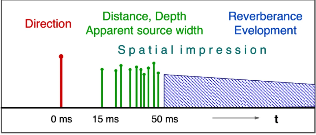
Der Einﬂuß von "frühem" und "spätem" Schall:

§  Direkter Schall → Aufschluß über Richtung der Schallquelle

§  Early reﬂections (nur wenige Reﬂexionen) → Aufschluß über Entfernung & "Breite" der Source

§  Late reﬂections (reverberations) → Informationen über den Raum

§  

Fazit: man muss eine große Zahl von Schall-Pfaden berechnen!

Figure 2: Influence of attributes on sound impression over time

2.1. Reflections and Reverb

Indirect sound portions allow for reproducing the recording space. The relation between direct and indirect sound determines the spatial attributes of a sound event. Figure 2 shows this interrelation. The natural pattern of early reflections occurring at a delay of 15 to 50 milliseconds plays a key role in spatial hearing. When it comes to recording, this portion of reflected sound deserves special attention as it critically affects attributes such as distance, depth, and spatial impression. The hearing takes spatial information from early reflections and converts it to a spatial event. With natural sound, the human ear performs this conversion spontaneously and with amazing robustness because that type of sound contains all properties of a reflection pattern in their original form. Key parameters include

 the timing structure in relation to direct sound

 levels and spectrums

 horizontal and vertical incidence directions

Imaging a spatial environment is realistic when the ear is able to recognize and interpret the features of the reflected sound – that is, when it “understands” the reflection pattern. Therefore, the reproduction must be absolutely consistent with a real spatial environment. The same applies to the spatial distribution of the early reflections’ incidence directions. Meeting this requirement using room microphones is hardly possible (see section 4) because one needs to keep acoustic crosstalk on the ambient-microphone channels as low as possible (approx. 10 dB at the most). A single reflection coming in from a specific direction – say, the top-right corner of the rear part of the hall – should be reproduced as such; it must not be picked up by the “wrong” mikes. This would be the case, for example, when using omnidirectional microphones in a room-microphone array.

The perception of distances and depth mostly depends on early reflections. This can be proven by simply adding pure early reflections (without the reverb) derived from a real room to a source that has been dryly recorded. The source is perceived as remote, which is in correspondence with the reflection pattern.

Perception is particularly stable when the reflections come in from the original directions of the upper half space. Reproducing depth requires careful handling of early reflections.

Adding appropriate reverb at a suitable level creates a natural sense of depth and realistic spatial impression /². Even with short reverb times, the virtual reproduction of these two attributes creates a realistic spatial impression. Increasing the reverb time, for example, by using concert-hall or church reverbs, adds another attribute of spatial hearing: the envelopment.

/ ² The term “spatial impression” refers to the effect of early reflections and early reverb on localization. Due to reverberation inside the room, the apparent source width (ASW) seems greater, and the source event appears to be “fuzzy” in time.

t 0 ms 15 ms

Direction Distance, Depth Apparent source width

Reverberance Evelopment

50 ms

S p a t i a l i m p r e s s i o n

t 0 ms 15 ms

Direction Distance, Depth Apparent source width

Reverberance Evelopment

50 ms

S p a t i a l i m p r e s s i o n

(9)

C C

Spiegelquellen-Methode ("image source")

§ 

Zur schnellen Berechnung der Reﬂexionspfade

§  

Idee: konstruiere für jede Schallquelle und jede Wand eine

"virtuelle" Schallquelle ("image source")

§ 

Länge des Strahls à Laufzeit,

#Reﬂexionen à Dämpfung

§  

Aufwand: O( n^.r )

n = # Schallquellen, r = # Wände.

§  

Probleme:

§  Alles neu berechnen,

wenn sich Quellen bewegen

§  Nur Reﬂexionseffekt

Listener

Source 1

2

3 4 S₁

S₂

S₃ S₄

(10)

C C

§ 

Beispiel (nicht alle Spiegelquellen eingezeichnet):

Source Listener

Spiegelquelle zweiten Grades Orig. Quelle

wird verdeckt

Listener auf der

"falschen" Seite der Wand

(11)

C C

Ray Tracing Methods

§ 

Verschieße Strahlen von Schallquelle (oder Listener).

§ 

Probleme:

§  Viele Strahlen "umsonst",

§  Listener besteht eigtl. aus 2 sehr kleinen Punkten im Raum

§  Wie ﬁndet man garantiert die Hauptpfade?

Source Listener

(12)

C C

Beam Tracing

§ 

Beam = ausgedehnter, sich aufweitender Strahl

§ 

Damit läßt sich viel vorausberechnen, zur Laufzeit Strahlrückverfolgung

§ 

Beam-Tracing:

1. Sortiere Polygone entlang Beam,

2. Für jedes Polygon, das Beam schneidet:

spalte Beam auf in 2 oder mehr,

bestimme Spiegelquelle für reﬂektierten Beam 3. Rekursion

(13)

C C

Source S

S'

S''

(14)

C C

Sound-Rendering mit Beams

§ 

Alle Beams berechnen: zu jedem Beam speichere:

§  zugehörige Quelle/Spiegelquelle;

§  spiegelndes Polygon;

§  Vater-Beam;

§  Anzahl Reﬂexionen;

§  ursprüngliche Quelle;

à "Beam tree".

§ 

Für gegebenen Listener:

1. Bestimme alle enthaltenden Beams,

2. Verfolge Strahlen zurück in Richtung der Quellen/Spiegelquellen über die Spiegelpolygone bis zum Ursprung mittels Image-Source-Methode, 3. Signale aufaddieren.

(15)

C C

Beschleunigung des Beam-Tracings

§ 

Wie macht man Beam-Tracing schnell ?

§ 

Idee: Berechne weitere Datenstruktur, die Szene in konvexe Zellen aufteilt.

§  Denn: ein Punkt in geschlossenem Polyeder "sieht" jedes Rand- Polygon;

§ 

Deﬁnition Zelle :

"Zelle" ist ein Volumen des Raumes, mit der Eigenschaft:

1. Das Volumen ist konvex;

2. Das Innere des Volumens enthält keine Polygone.

§ 

Zu jeder Zelle speichere:

§  Nachbarzellen

("cell adjacency graph"),

§  Rand-Polygone.

A B

C D

(16)

C C

Beam-Tracing mit Zellen

Gegeben Quelle, wie wird Beam "verschossen" und "beschnitten"?

1. 

Bestimme Zelle, in der der Beam anfängt

(entweder von Punkt innerhalb der Zelle, oder vom Rand).

2. 

Für jedes Polygon am Rand: generiere gespiegelten Beam, falls Polygon getroffen, und schneide Beam ab.

3. 

Falls etwas "übrigbleibt" vom Beam, beginne wieder von vorne in der Nachbarzelle.

4. 

Rekursion mit den gespiegelten und den "übriggebliebenen"

Beams.

(17)

C C

Gesamtsystem

Dekomposition in Zellen

Beam Tracing

Strahl- rückverfolgung

Signal-Addition Geometrie

Position/Richtung der Schallquellen

Position/Richtung des Empfängers

Audiosignal

Räumliches Audiosignal Zell-Graph Beam-Tree

Strahlen

(18)

C C

§ 

Eigenschaften des Algorithmus':

§  Schnell

§  Auch Beugung schnell berechenbar

§  Gut parallelisierbar

(19)

C C

(20)

C C

Exkurs: Monte-Carlo-Integration

§ 

Aufgabe: bestimmtes Integral berechnen

(wobei f zu "schwierig" zum analytischen Berechnen des unbestimmten Integrals sei)

§ 

Triviale numerische Näherung: f auf einem Gitter auswerten

wobei

§ 

Wenn , dann geht

§ 

Alternative Betrachtung:

d.h., jedes wird mit gewichtet E =

Z _b

a

f (x) dx

E_N =

XN i=1

h·f (a + i·h) h = ^{b a}_N

N ! 1 E_N ! E

E_N = (b a) XN

i=1

1

Nf (x_i) ,x_i = a + i·h

f (x_i) _N¹

(21)

C C

§ 

Das selbe funktioniert auch für mehrdimensionale Integrale, d.h., dass :

wobei die x_i (insgesamt N Stück) wieder auf einem regelmäßigen Gitter innerhalb von Ω angeordnet sind

§ 

Probleme:

§  Aufwand steigt exponentiell mit d, weil Vol(Ω) = Seitenlänge^d

§  Sampling von f ist schwierig, falls das Gebiet Ω eine nicht-kanonische Form hat

§  

Lösung: Monte-Carlo-Integration = sample f an zufälligen, gleichverteilten Positionen x_i:

f : R^d ! R E =

Z

⌦

f (x) dx ⇡ Vol(⌦) XN

i=1

1

N f (xi)

E_N = (b a) XN

i=1

1

N f (x_i)

(22)

C C

§ 

Wie wahrscheinlich ist es, dass E_N "nah" bei E liegt?

§ 

Beobachtung: wenn die {x_i} zufällig gezogen sind, ist auch E_N eine Zufallsvariable, die eine bestimmte Wahrscheinlichkeits- dichtefunktion haben muß

§ 

Zentraler Grenzwertsatz (central limit theorem) sagt:

wenn N groß ist, dann folgt E_Nungefähr der Gauss'schen

Normalverteilung, mit Mittelwert E, und Standardabweichung

§ 

Mit W'keit 0.95 liegt E_N im Intervall [E-σ_N,E+σ_N]

§ 

Die Standardabweichung σ_Nsagt also etwas über die Unsicherheit unserer Schätzung von E aus

N2 =

b a N

PN

i=1 f ²(xi) E_N² N 1

(23)

C C

§ 

Vorteil von Monte-Carlo-Integration:

§  Man kann N beliebig steuern (muss nicht mehr n^d sein)

§  Beliebige Gebiete lassen sich leicht sampeln &

integrieren, falls der Test x ∈ Ω einfach ist, z.B.

Integration über eine Kugel

§ 

Weitere Probleme:

der Beitrag manchener / vieler Sample-Punkte x_i zu kann sehr gering sein

§ 

Ziel: versuche nur dort zu sampeln, wo f groß ist

➙  Importance Sampling

P_N

i=1 1

Nf (x_i)

(24)

C C

§ 

Beispiel:

§  

Der größte Beitrag kommt von x-Werten nahe 1

§  

Wähle Sample-Stellen nicht uniform, sondern gemäß Dichtefunktion p(x), z.B.

§  

Frage: wie muß das Integral geschrieben werden, um den Bias (hier: "Vorliebe" für

bestimmte Sample-Region) zu kompensieren?

E = Z 1

0

3x² dx

( ) 3 2

f x = x

p(x)=2x

p(x) = 2x

(25)

C C

§ 

Eine (eindimensionale) Plausibilitätsbetrachtung:

§  Betrachte numerische Integration mit Rechteck-Regel:

§  Ein Δx_i = Kehrwert der lokalen Dichte der Sample-Punkte:

EN =

XN

i=1

xi·f (xi)

xi = b a

N · 1 p(x_i)

Größeres p

→ mehr Sample-Punkte

→ kleineres Δxi

x1

Δ Δx₂ Δx₃ ^… Δx_n

(26)

C C

§ 

MC-Integration mit Importance-Sampling:

wobei die x_i zufällig gemäß der Wahrscheinlichkeitsdichtefunktion p(x) gewählt werden

§ 

Mehrdimensionale funktioniert es ganz analog:

E_N = b a N

XN i=1

f (x_i) p(xi)

EN = Vol(⌦) N

XN

i=1

f (x_i) p(x_i)

(27)

C C

Stochastisches Sound-Rendering

§ 

Szenen mit vielen Schallquellen (z.B. 100k)

§  Durch Spiegelquellenmethode

§  Stadium, Fußgängerzone, …

§ 

Mixing

läßt sich nicht mehr für alle mit 40 kHz durchführen

§ 

Wähle k Samples aus n:

schätze Gesamtsignal s(t) durch:

(28)

C C

Importance Sampling

§ 

Wahl der Wahrscheinlichkeiten:

§  Optimal wäre:

§  Vereinfachung:

§  

Dynamische Veränderungen in der Szene:

§  Listener bewegt sich

§  Schallquelle bewegt sich (oder rotiert und Abstrahlcharakteristik ist nicht kugelförmig)

§  Occluder oder Reﬂektoren bewegen sich

§  Die a_i ändern sich, damit auch die p_i

(29)

C C

Dynamisches Importance Sampling

1.  Volles Resampling:

§  Schätzung ŝ ist nicht exakt

§  Umschalten auf neues Sample-Set hörbar

2.  Stochastic diffusion:

§  Wechsle pro Zeiteinheit nur einen gewissen Anteil des Sample-Sets

§  Fade-out, dann ersetzen durch neue zufällige Quelle, dann Fade-in

§  Weniger, aber immer noch Artefakte

3.  Adaptive diffusion:

§  Passe Änderungsrate des Sample-Sets der Änderungsrate der a_i an

§  Falls sich mehr als ε geändert hat:

-  Fall "zu klein": fade-out, ersetzen, fade-in

-  Fall "zu groß": anderes Sample ausfaden und ersetzen durch zufälliges Sample

§  Problem: immer noch O(n) Zeit, da Auswahl gemäß p_i irgendeine Form der Durchmusterung benötigt

(30)

C C

Hierarchisches Sampling

§ 

Für statische Szenen

§ 

Octree über Schallquellen:

§  Repräsentant = einer der Repräsentanten der 8 Kinder (Wahrscheinlichkeit ~ Volumen)

§  Volumen des Repräsentanten = Summe der Volumen der Kinder Orig. Quellen Repräsentant

(31)

C C

Prioritätsgesteuerte Traversierung

§  Priorität = Lautstärke des Repräsentanten x Dämpfung

§  Algorithmus:

repeat

hole Top aus Queue

füge Top zur Liste der k Samples füge Kinder von Top in Queue

until k Elemente in Liste

§  Laufzeit: O(k log k)

§  Implementiert Importance Sampling

§  Und Stratiﬁzierung ("stratiﬁcation" = "gleichmäßigere Auswahl")

§  Nachteile:

§  Nur Empfängercharakteristik und Dämpfung durch Distanz

§  Sichtbarkeit und Emissionscharakteristik werden ignoriert

§  Lösung:

§  Wähle 10,000 Kandidaten mit hierarchischem Sampling

§  Wähle daraus mit dynamischem Sampling 100-1000 Samples

(32)

C C

13 versch. Soundtracks, zufällige Phasenverschiebung, 16 bit, 44.1 kHz, Mono;

Mixer erzeugt Stereo.

Sekundärquellen durch Photon-Tracing erzeugt (diffuse Reﬂexion)

(33)

C C

Sekundärquellen durch Spiegelquellenmethode

(34)

C C

Audio-Processing on the GPU

§  Aufgaben des Mixer:

§  Audiodaten verschieben (Zeitverzögerung)

§  Strecken oder Stauchen (Dopplereffekt)

§  n Frequenzbänder gewichten und aufsummieren (pro Schallquelle)

§  Idee: verwende GPU

§  Audiodaten = 1D-Textur (4 Frequenzkanäle → RGBA)

§  Texturkoord.verschiebung = Zeitverzögerung

§  Farbtransformation = Frequenzmodulation

§  Skalierung der Texturkoord. = Dopplereffekt

Gestreckte Textur

Neues Signal (Dopplerv.)

(35)

C C

§  HRTF ("head-related transfer function"

= Empfängercharakteristik) = Cubemap

§  Mixen = 4D-Skalarprodukt

§ 

Vergleich:

§  SSE-Implementierung auf 3 GHz Pentium 4

§  GPU-Implementierung auf GeForce FX 5950 Ultra, AGP 8x

§  Audio-Processing: Frames der Länge 1024-Samples, 44.1 kHz, 32-bit ﬂoating point.

§  Resultat:

-  GPU ca. 20% langsamer,

-  Zukünftige GPUs evtl. ca. 50% schneller -  Bus-Transfer unberücksichtigt