Virtual Reality & Physically-Based Simulation

(1)

Virtual Reality &

Physically-Based Simulation

Haptics

G. Zachmann

University of Bremen, Germany

cgvr.cs.uni-bremen.de

(2)

G. Zachmann Virtual Reality & Simulation WS 24 January 2018 Haptics & Force-Feedback 6

Some Technical Terms

§ Haptics = sense of touch and force (greek haptesthai = berühren)

§ Special case: force feedback

§ What is to be rendered:

§ Forces on the user's hand / arm (= haptic "image" of objects)

§ Haptic texture of surfaces (roughness, grain, friction, elasticity, ...)

§ Shape of objects by way of touching/feeling

(3)

Applications

§ Training of minimally invasive surgery (surgeons rather work by feeling, not seeing)

§ Games? Can increase presence significantly (self-presence, social presence, virtual object presence)

§ Industry:

§ Virtual assembly simulation (e.g., to improve worker's performance / comfort when assembling parts)

§ Styling (look & feel of a new product)

- Ideally, one would like to answer questions like "how does the new design of the

product feel when grasped?"

(4)

Example Application: Minimally Invasive Surgery

(5)

Another Application: Assembly Simulation

DLR: A Platform for Bimanual Virtual Assembly Training with Haptic Feedback in Large Multi-Object Environments

(6)

A Collection of Force Feedback Devices

CyberForce CyberForce

Sarcos

(movie)

Phantom

(movie)

Force Dimension

(7)

Scale-1 by Haption

(8)

Tsukuba

Spidar

(movies)

Maglev (Bytterfly Haptics)

(9)

Devices with Force Feedback via Wires (Spidar Variants)

Two-Handed Multi-Fingers Haptic Interface Device: SPIDAR-8

(10)

G. Zachmann Virtual Reality & Simulation WS 24 January 2018 Haptics & Force-Feedback 15 INCA 6D von Haption

(11)

Tactile Displays

CyberTouch

Fe ele x

SmartTouch

AU RA IN TE RAC TO R

GloveOne

(12)

G. Zachmann Virtual Reality & Simulation WS 24 January 2018 Haptics & Force-Feedback 17 NormalTouch & TextureTouch, 2016, Microsoft

(13)

Haptic Feedback via Interference of Ultrasound

(14)

Haptoclone

micro mirror array 1992 phase-controlled ultrasound array Depth sensor for objs

(15)

Motion Platforms

Flogiston

(Not Really Force-Feedback)

BlueTiger

MPI Tübingen

(16)

The Special Problem of Force-Feedback Rendering

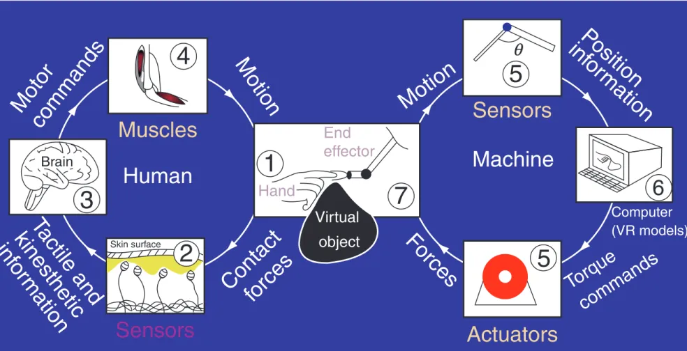
relationship between the machine and the human in a haptics-enabled VE. The central box contains the tip of a haptic interface device which the user grasps.

The left-hand loop of the picture shows the human interaction with the device. The human senses, through his/her contact with the device, forces to which he/she responds by providing motor signals that move his/her hand, which in turn affects the device. As shown in the right-hand loop, the com- puter attached to the device senses the movement of the device and responds by sending commands that create the forces the device applies on the human.

Both the human and the computer systems have sen- sors (receptors and encoders), processors (brain and computer), and actuators (muscles and motors). That is, the machine haptic system mirrors and extends the human haptic system.

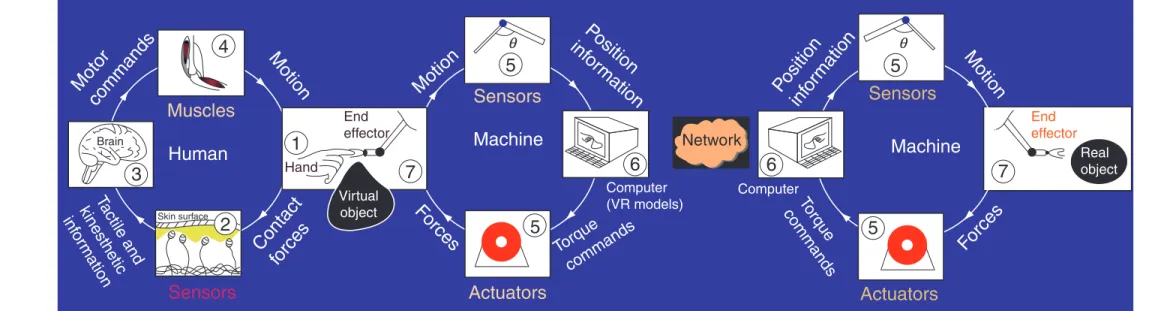
In the case of TO systems, the haptic interface is connected to a computer as previously discussed, but that computer, in turn, is connected to another com- puter, either directly or over a network such as the Internet, and haptic signals are sent back and forth between the two. This allows a user of the first com- puter to interact with a real environment through an interface device such as a robot that is connected to

the second computer. This kind of TO system is sum- marized in Figure 2.

More complex haptic interactions are possible with a system that combines VEs with TO to enable two- way interactions across a network. One case of this was in 2002 when people at the MIT Touch Lab shook hands, transatlantically, with people at University College, London. In the future, haptic interactions at a distance will be prevalent, powerful, and important.

These systems bring with them several new technical challenges (e.g., dealing with the latency of the trans- mitted signals) as well as new kinds of applications.

However, for the sake of ease of explication, this article is confined to the more simply explained VE paradigm until the applications section, in which emerging practical uses of VE and TO systems are discussed together. The section above brings out at least two reasons why a neuroscientist might be interested in machine haptics. First, machine haptics provides a par- ticular way of doing neuroscience: having unprece- dented control over touch stimuli displayed through haptic interfaces allows experimentation with the human haptic sensory system, the human motor sys- tem, and interactions between the two, as well as with other sensory systems such as vision and hearing.

Second, machine haptics provides an application area for neuroscience: bringing neuroscientific knowledge of the human haptic system to engineering design will help create improved haptic interfaces in the future.

The development of engaging, compelling haptic inter- faces will require an understanding of the roles played by the mechanical, sensory, motor, and cognitive sub- systems of the human haptic system. Therefore, machine haptics, both as a research topic and as a branch of engineering, in its search to provide natural touch interfaces for computers, requires an under- standing of human haptics and an understanding of the psychology of human–machine and human–

human interactions in VE and TO systems, as well as the technological questions of hardware and software.

Motor

commands

Tactile and kinesthetic inf or

mation

Human

Motion

Contact forces Sensors

Machine

Fo rces

Torque

commands

Computer (VR models)

Po sition inf or

mation

Muscles Sensors

Actuators

Brain

4

3

1 5 ^q

2

7

5

6

Skin surface

Virtual object

End effector Hand

Figure 1 Human–machine haptic interaction in virtual environments.

Sensors

6

5 7 Motion

Forces Po sition

inf or mation

To rq commands ue

Machine

Actuators

Computer

Human Machine

Forces

Torque

commands

Muscles Sensors

Actuators

Brain

4

1

5 q

5

2

7 5 5

6 6

3 Motor

commands

Motion

Position inf or mation

Contact forces

Ta ctile and kinesthetic inf or

mation

Virtual object

End effector Hand

Skin surface

Sensors

Computer (VR models)

Network

Real object End

effector

q

Figure 2 Human–machine haptic interaction in teleoperated environments.

590 Machine Haptics

M A Srinivasan & R Zimmer: Machine Haptics.

New Encyclopedia of Neuroscience, Ed: Larry R. Squire, Vol. 5, pp. 589-595, Oxford: Academic Press, 2009

(17)

… and that of Telepresence

relationship between the machine and the human in a haptics-enabled VE. The central box contains the tip of a haptic interface device which the user grasps.

The left-hand loop of the picture shows the human interaction with the device. The human senses, through his/her contact with the device, forces to which he/she responds by providing motor signals that move his/her hand, which in turn affects the device. As shown in the right-hand loop, the com- puter attached to the device senses the movement of the device and responds by sending commands that create the forces the device applies on the human.

Both the human and the computer systems have sen- sors (receptors and encoders), processors (brain and computer), and actuators (muscles and motors). That is, the machine haptic system mirrors and extends the human haptic system.

In the case of TO systems, the haptic interface is connected to a computer as previously discussed, but that computer, in turn, is connected to another com- puter, either directly or over a network such as the Internet, and haptic signals are sent back and forth between the two. This allows a user of the first com- puter to interact with a real environment through an interface device such as a robot that is connected to

the second computer. This kind of TO system is sum- marized in Figure 2.

More complex haptic interactions are possible with a system that combines VEs with TO to enable two- way interactions across a network. One case of this was in 2002 when people at the MIT Touch Lab shook hands, transatlantically, with people at University College, London. In the future, haptic interactions at a distance will be prevalent, powerful, and important.

These systems bring with them several new technical challenges (e.g., dealing with the latency of the trans- mitted signals) as well as new kinds of applications.

However, for the sake of ease of explication, this article is confined to the more simply explained VE paradigm until the applications section, in which emerging practical uses of VE and TO systems are discussed together. The section above brings out at least two reasons why a neuroscientist might be interested in machine haptics. First, machine haptics provides a par- ticular way of doing neuroscience: having unprece- dented control over touch stimuli displayed through haptic interfaces allows experimentation with the human haptic sensory system, the human motor sys- tem, and interactions between the two, as well as with other sensory systems such as vision and hearing.

Second, machine haptics provides an application area for neuroscience: bringing neuroscientific knowledge of the human haptic system to engineering design will help create improved haptic interfaces in the future.

The development of engaging, compelling haptic inter- faces will require an understanding of the roles played by the mechanical, sensory, motor, and cognitive sub- systems of the human haptic system. Therefore, machine haptics, both as a research topic and as a branch of engineering, in its search to provide natural touch interfaces for computers, requires an under- standing of human haptics and an understanding of the psychology of human–machine and human–

human interactions in VE and TO systems, as well as the technological questions of hardware and software.

Motor commands

Tactile and kinesthetic infor

mation

Human

Motion

Contactforces Sensors

Machine

Forces

Torque commands

Computer (VR models)

Position information

Muscles Sensors

Actuators

Brain

4

3

1

5^q

2

7

5

6

Skin surface

Virtual object End effector Hand

Figure 1 Human–machine haptic interaction in virtual environments.

Sensors

6

5

7 Motion

Forces Position

information

Torq commandsue

Machine

Actuators

Computer

Human Machine

Forces

Torque commands

Muscles Sensors

Actuators

Brain

4

1

5 q

5

2

7

5 5

6 6

3 Motor

commands

Motion

Position infor

mation

Contact forces Tactile and

kinesthetic infor

mation

Virtual object End effector Hand

Skin surface

Sensors

Computer (VR models)

Network

Real object End

effector

q

Figure 2 Human–machine haptic interaction in teleoperated environments.

590 Machine Haptics

M A Srinivasan & R Zimmer: Machine Haptics.

New Encyclopedia of Neuroscience, Ed: Larry R. Squire, Vol. 5, pp. 589-595, Oxford: Academic Press, 2009

(18)

Putting the Human Haptic Sense Into Perspective

§ Amount of the cortex devoted to processing sensory input:

§ Haptic sense is our

second-most important sense

Sensory Input Amount of cortex / %

Visual 30

Haptic 8

Auditory 3

Somatosensory cortex (touch)

Visual cortex

Auditory cortex

Gustatory cortex (taste)

Olfactory

cortex

(19)

The Human Tactile Sensors

§ There are 4 different kinds of sensors in our skin:

Mechanoreceptors

• Temporal Properties (adaptation)

• Rapidly adapting fibers (RA) found in Meissner receptor and Pacinian corpuscle - fire at onset and offset of stimulation

• Slowly adapting fibers (SA) found in Merkel and Ruffini receptors - fire continuously as long as pressure is applied

SA1

SA2

RA2

RA1

Surface

Deep

Epidermis Dermis

Subcutaneous fat

Ruffini cylinder

Pacini corpuscle

Meissner corpuscle Merkel discs

Duct of sweat gland

(20)

§ Their characteristics:

§ Ruffini & Merkel: slowly adapting (SA)

⟶ fire as long as the stimulus persists

§ Meissner & Pacini: rapidly adapting (RA)

⟶ fire only at onset and offset of stimulus

Mechanoreceptors

• Temporal Properties (adaptation)

• Rapidly adapting fibers (RA) found in Meissner receptor and Pacinian corpuscle - fire at onset and offset of stimulation

• Slowly adapting fibers (SA) found in Merkel and Ruffini receptors - fire continuously as long as pressure is applied

SA1

SA2

RA2

RA1

Surface

Deep

Ruffini cylinder

Pacini corpuscle

Meissner corpuscle Merkel discs

Merkel Meissner

Ruffini Pacini

slow fast

Adapting Rate

Re sp on se t o vi b ra ti on fr eq u en cy lo w hi g h Lo ca tio n in S kin

su rfa ce deep

(21)

Some Human Factors Regarding Haptics

§ Human factors of the tip of a finger:

§ Precision = 0.15 mm regarding the position of a point

§ Spatial acuity = 1 mm (i.e., discrimination of 2 points)

§ Detection thresholds ("there is something"):

0.2 micrometers for ridges; 1-6 micrometers for single points

§ Temporal resolution: 1 kHz (compare that to the eye!)

§ Kinaesthetic (proprioceptive) information:

§ Obtained by sensors in the human muscles

§ Can sense large-scale shapes, spring stiffness, …

§ Human factors:

- Acuity: 2 degrees for finger, 1 degree for shoulder

- 0.5-2.5 mm (finger)

(22)

§ Time until a reflex occurs:

§ Reflex by muscle: 30 millisec

§ Reflex through spinal cord: 70 millisec

§ Voluntary action: ?

§ The bandwidth of forces generated by humans:

§ 1-2 Hz for irregular force signals

§ 2-5 Hz when generating periodic force signals

§ 5 Hz for trained trajectories

§ 10 Hz with involuntary reflexes

§ Forces of hand/arm:

§ Max. 50-100 N

§ Typ. 5-15 N (manipulation and exploration)

§ Just noticeable difference (JND) = = 0.1 (10%) ^F

^ref

_F ^F

^comp

ref

(23)

Simulation Factors

§ Sensation of stiffness/rigidity: in order to render hard surfaces, you need >1 N/mm ( better yet 10 N/mm)

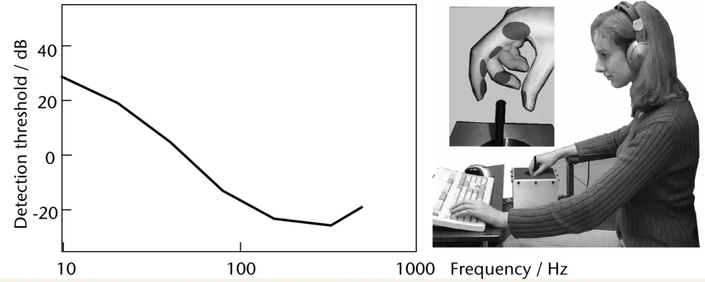
§ Detection threshold for vibrations:

§ Simulation must run at Nyquist frequency ⟶ in order to generate haptic signals with 500 Hz, the simulation loop must run at 1000 Hz

Frequency / Hz

De te ct io n th re sh ol d / d B

-20 0 20 40

10 100 1000

Apex, North Carolina) were fastened between the minishaker and the stylus (see Fig. 1) through adapter plates. The bottom adapter below the force sensor was fastened to the threaded hole connected to the shaker actuator. The top adapter holding the accelerometer was connected to the stylus by means of a set screw. The apparatus was placed on several rubber pads inside a metal enclosure that sat above a table. The stylus protruded through a hole on top of the enclosure so that it could be grasped by a hand. An arm rest was built to support the participant's elbow and upper arm (see Fig. 2).

Figure 1. Shaker assembly with one of the side panels removed.

The apparatus was controlled by a data acquisition board (Nation Instruments PCI-6229, Austin, Texas) with an open- loop control scheme. Command signals were generated from the board that first passed through a 16-bit Digital-to-Analog converter and then through a high-bandwidth linear audio power amplifier (model LVC 608, AE Techron Inc., Elkhart, Indiana) whose output was used to excite the minishaker vertically (along the length of the stylus). The acceleration and force data were captured by two 16-bit Analog-to-Digital converters at a sampling rate of 10 kHz. The acceleration data were integrated once and twice to obtain velocity and position estimates, respectively, for further analysis of detection threshold and mechanical impedance.

A calibration routine was performed to develop an input- output relationship for the apparatus at test frequencies by fitting a least-square straight-line through the controlled vibration input (in volts) and measured position data (in mm) at several amplitude levels. The routine was performed without loading the apparatus and with the human hand load.

The input-output relation was well represented by a straight- line (r

²

>0.99) in the operating range with a significant (p<0.0001) slope at each test frequency. The estimated slope and intercept of the straight-line fit were used to compensate the command signal in order to reach the desired output vibration levels. Force and position measurements were

transformed into the frequency domain by taking the Fast Fourier Transform (FFT) of the measured data. Mechanical impedance was estimated by the ratio of the force/velocity amplitudes, F/v, and was plotted against frequency under unloaded condition. The ratio was highly linear (r

²

>0.99) and a slope of 20 dB/decade indicated that only the inertial element was dominant between the measured force and position data (i.e., ^F ^mx ) under unloaded condition.

B. Participants

Five males and five females (age 22-40 years old, average 28 years old) participated in the study. Nine out of the ten participants were right-handed by self-report. Five of the participants had either participated in other haptic perception experiments in our laboratory before and/or were involved in developing the hardware/software system used in the present study. They were regarded as “experienced” users of force- feedback and vibrotactile haptic devices. The rest of the participants were regarded as “inexperienced.”

C. Procedure

The participant sat comfortably in front of a computer monitor with the dominant hand holding the stylus. The participant’s elbow and forearm rested on the arm rest that supported a neutral wrist position (see Fig. 2). The participant was instructed to hold the stylus like holding a pen or the stylus of a PHANToM force-feedback device. Some participants practiced by using the PHANToM device (not shown) for a few minutes prior to the experiment. When the stylus was held as instructed, the vibrations transmitted through the stylus were mostly tangential to the skin in contact. The areas of the skin touching the stylus are illustrated by shaded ovals in the inset of Fig. 2.

Figure 2. Experimental setup.

Seven test frequencies (10, 20, 40, 80, 160, 320, and 500 Hz) were used. They were chosen to be equally spaced on a logarithmic scale except for the highest frequency. The order of the test frequencies was randomized for each participant.

The duration of the stimulus was fixed at 1 sec with Hanning

windowing (100-msec rise and fall) to reduce transient effects.

(24)

Rule of Thumb: Hz Update Rate Needed for Haptic Rendering

§ An Experiment as "proof":

§ Haptic device with a pen-like handle and 3 DOFs

§ The virtual obstacle = a flat, infinite plane

§ Task: move the tip of the pen along the surface of the plane (tracing task)

§ Impedance-based rendering (later)

§ Stiffness = 10000 N/m, coefficient of friction = 1000 N/(m/sec)

§ Haptic sampling/rendering frequencies: 500 Hz, 250 Hz, 167 Hz

EXPERIMENT Experiment(l)

As a preliminary experiment, a tracing task by conventional approach(Fig.1) was carried out. The operator touched on a stiff wall( K = 10000 N/m, B = 1000 N/(m/see)) which was placed at X = -100 mm. Three sampling intervals(T), 2mSec (lD=5OOHz), 4mSec

(ln=25OHz) and 6mSec (l/r=167Hz)) were prepared for the experiment.

The trajectories projected on x-y plane are shown in Fig.13. The dots show the movement of the tip of the operator’s finger at each sampling time. Fig.l3(a) indi- cates that the operator could touch and trace on the surface smoothly. However, when the sampling intervals were 4mSec and 6mSec, unpleasant vibration was ce- curred (Fig.13 (b),(c)). From the result, it is confirmed that sampling rate of Impedance control should be greater than 5OOHz for the implementation of stiff objects.

Y(md 70 - 60 - 50 -

40 - 30 -

. . . P--~-““‘- ...

dry ... . f +-

... ... ...

-101 -100 -99 -98 -91

x(md (a) Sampling Interval : 2 mSec ( 500 Hz )

,. . . . . . . * * D-

. . . 2otLdhdbZ

-102 -101 -100 -99 -98

xwd (b) Sampling Interval : 4 m&c ( 2.50 Hz )

yt-1 50 -

40 -

30 -

20 -

~. . .

. “’

4

lOI._ ’ I I I

-102 -101 -100 -99 -98

x(-) (c) Sampling Interval : 6 mSec ( 167 Hz )

Figure 13: Tracing on the stiff wall placed at x = -100 by conventional method

Stiffness and viscosity are 10000 N/m and 1000 N/(mkec) respectively.

207

Y(md 70 - 60 - 50 -

40 -

30 -

. . . P--~-““‘- ...

dry ... . f +-

... ... ...

-101 -100 -99 -98 -91

,. . . . . . . * * D-

. . . 2otLdhdbZ

_-102 _-101 _-100 _-99 -98

yt-1 50 -

40 -

30 -

20 -

~. . .

. “’

4

lOI._ ’ I I I

-102 -101 -100 -99 -98

207

Y(md 70 -

60 - 50 -

40 -

30 -

. . . P--~-““‘- ...

dry ... . f +-

... ... ...

-101 -100 -99 -98 -91

,. . . . . . . * * D-

. . . 2otLdhdbZ

-102 -101 -100 -99 -98

yt-1 50 -

40 -

30 -

20 -

~. . .

. “’

4

lOI._ ’ I I I

-102 -101 -100 -99 -98

207

Position of the tip at each sampling time

40 $

Figure 7: Structure of mechanism of SPICE

Figure 8: General view of SPICE

+++ ++ ^{+t l +} A+

Force Command (N)

Figure 10: Force command and output of SPICE Y direction at center of work space

IRIS 420,‘VGX

SPICE

Figure 11 Structure of the controller r

Figure 9: Distribution of GIE Figure 12: General view of experimental system

206

1000

Tip direction

167 Hz 250 Hz 500 Hz

(25)

Haptic Textures

§ Texture = fine structure of the surface of objects (= micro- geometry); independent of the shape of an object (= macro- geometry)

§ Haptic textures can be sensed in two ways by touching:

§ Spatially

§ Temporally (when moving your finger across the surface)

§ Sensing haptic textures via force-feedback device:

as you slide the tip of the stylus along the surface,

texture is "transcoded" into a temporal signal, which is then output on the device (e.g., use IFFT to create the signal)

4.1 Experiment Design

4.1.1 Apparatus. The PHANToM force- reflecting device was used for both texture rendering and data collection. The position of the tip of the stylus, p(t), was measured using the position-sensing routines in the GHOST library provided with the PHANToM.

These routines read the optical encoders to sense joint angles of the PHANToM and converted them to a posi- tion of the stylus tip in the world coordinate frame.

For force and acceleration measurement, the PHAN- ToM was instrumented with two additional sensors. A triaxial force/torque (F/T) sensor (ATI Industrial Au- tomation, Apex, NC; model Nano 17 with temperature compensation) was used to measure force delivered by the PHANToM, f(t). In order to minimize the struc- tural change to the PHANToM, a new link with a built-in interface for the F/T sensor was fabricated to replace the last link (i.e., the link closest to the stylus) of the PHANToM (see Figure 7). The new link was of the same length as the original one, but weighed 60 g

(13%) more. Force data were transformed into the stylus coordinate frame. The origin of the stylus coordinate frame was always located at the tip of the stylus (i.e., p(t)), and its z-axis coincides with the cylindrical axis of the stylus (see Figure 1).

Acceleration of the stylus was captured with a triaxial accelerometer (Kistler, Blairsville, PA; model 8794A500).

The accelerometer was attached through a rigid mount that was press-fitted to the stylus. The attachment

added 11.8 g to the weight of the stylus. Acceleration measurements, a(t), were also taken in the stylus coordi- nate frame.

The effects of the sensor attachments on the device performance were investigated in terms of apparent in- ertia at the PHANToM stylus. We measured the tip in- ertia of the original and instrumented PHANToM

devices along paths that passed the origin of the PHAN- ToM coordinate frame. Two paths were chosen to be parallel to one of the axes of the PHANToM coordinate frame, differing in the direction of tip movement during the measurements (a total of six paths). The results are summarized in Table 3. It turned out that the tip inertia along the y-axis was affected most significantly by the the addition of the two sensors. In particular, the appar- ent tip inertia in the !y direction (the direction of grav- ity) was reduced by 139.4 g. This was due to the fact that the additional sensor weight increased the effect of gravity on the corresponding tip inertia. The inertia along other directions changed in the range 13.8 –29.4 g, and were therefore much less affected by the addi- tional sensor weight. Since the forces used in our experi- ments for rendering textured surfaces were confined in the x-z plane, we concluded, based on these measure- ments, that the instrumented PHANToM was able to reproduce the stimuli that led to perceived instability during the psychophysical experiments conducted ear- lier.

4.1.2 Subjects. Two subjects participated in the measurement experiment (one male, S1, and one fe- male, S4). Their average age was 33 years old. Both are right-handed and report no known sensory or motor abnormalities with their upper extremities. Only S1 had participated in the previous psychophysical experiments.

Both subjects were experienced users of the PHAN- ToM device. They were preferred over naive subjects because our experiments required the subjects to place or move the stylus in a particular manner in order to maintain well-controlled conditions during data collec- tion.

4.1.3 Experimental Conditions. A total of

seven experimental conditions was employed (see Table Figure 7. The PHANToM instrumented with a triaxial F/T sensor

and an accelerometer.

406 PRESENCE: VOLUME 13, NUMBER 4

(26)

A Frequent Problem: "Buzzing"

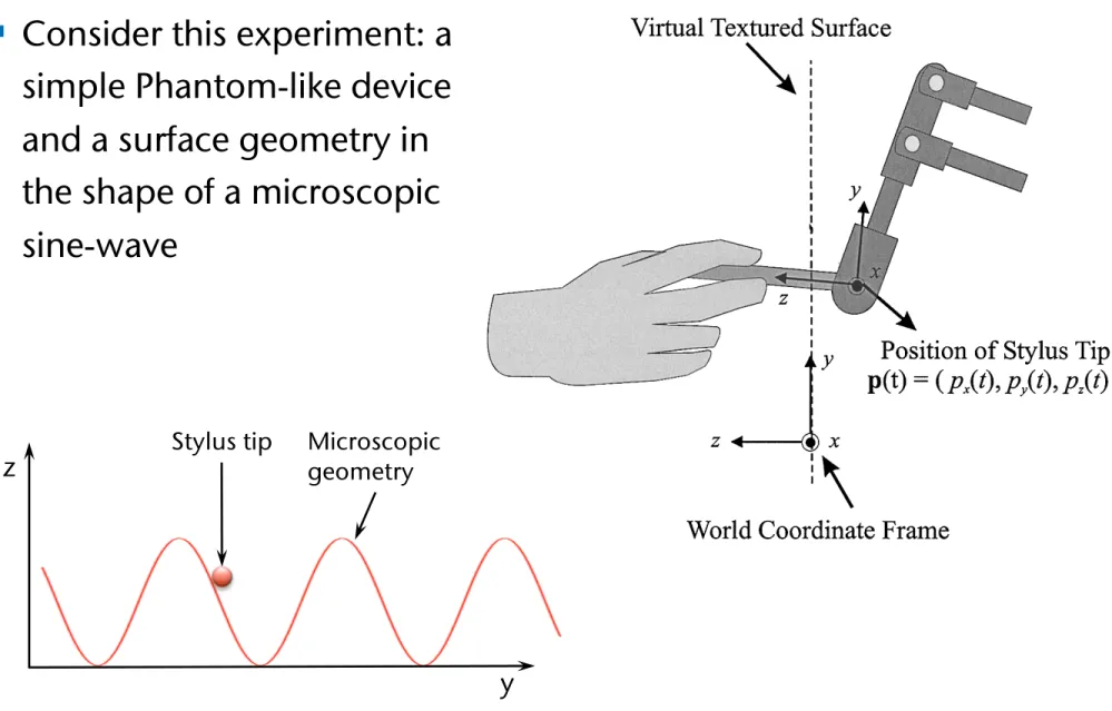
§ Consider this experiment: a simple Phantom-like device and a surface geometry in the shape of a microscopic sine-wave

length, respectively (see Figure 2). Sinusoidal gratings have been widely used as the basic building blocks for textured surfaces for studies on haptic texture percep- tion (Lederman et al., 1999; Weisenberger et al., 2000).

They have also been used as the basis of a function set for modeling real haptic textures (Wall & Harwin, 1999).

2.2 Texture Rendering Method

Two basic texture rendering methods were em- ployed in the current study. Both methods use a spring

model to calculate the magnitude of the rendered force as K ! d(t), where K is the stiffness of the textured sur- face, and d(t) is the penetration depth of the stylus at time t (see Figure 2). The penetration depth is calcu- lated as follows:

d!t" ! ! ^A ^sin ^!2# ^p

x

!t/L"" ⁰ $ A % p

_z

!t" ^if if ^p p

^z_z

^!t" !t" ^" & ⁰ 0 , (1) where p(t) # (p

_x

(t), p

_y

(t), p

_z

(t)) is the position of the tip of the stylus.

The two methods differ in the way the force direc- tions are rendered. The first method, introduced by Massie (1996), renders a force F

_mag

(t) with a constant direction normal to the underlying flat wall of the tex- tured surface. The second method, proposed by Ho et al. (1999), renders a force F

_vec

(t) with varying directions such that it remains normal to the local microgeometry of the sinusoidal texture model. Mathematically,

F

mag

!t" ! Kd!t" n

W

, (2)

F

vec

!t" ! Kd!t" n

T

!p!t"" , (3)

where n

_W

is the normal vector of the underlying flat wall, and n

_T

(p(t)) is the normal vector of the textured surface at p (t). Both methods keep the force vectors in the horizontal plane (zx plane in Figure 1), thereby eliminating the effect of gravity on rendered forces.

The two texture rendering methods are natural exten- sions of virtual flat wall rendering techniques. Perceptu- ally, they are very different: textures rendered by F

_vec

(t) feel rougher than those rendered by F

_mag

(t) with the same texture model. Textures rendered by F

_vec

(t) can also feel sticky sometimes.

2.3 Exploration Mode

An exploration mode refers to a stereotypical pat- tern of the motions that humans employ to perceive a certain object attribute through haptic interaction (Le- derman & Klatzky, 1987). In our experiments, we tested two exploration modes, free exploration and stroking, to examine the effect of user interaction patterns on in- stability perception. In the free exploration mode, sub- jects were allowed to use the interaction pattern that

Figure 1. An illustration of the virtual textured surfaces and the two coordinate frames used in our experiments. Position of the stylus tip was always measured in the world coordinate frame.

Figure 2. An illustration of the parameters used in texture rendering.

398 PRESENCE: VOLUME 13, NUMBER 4

Stylus tip

z

y

Microscopic

geometry

(27)

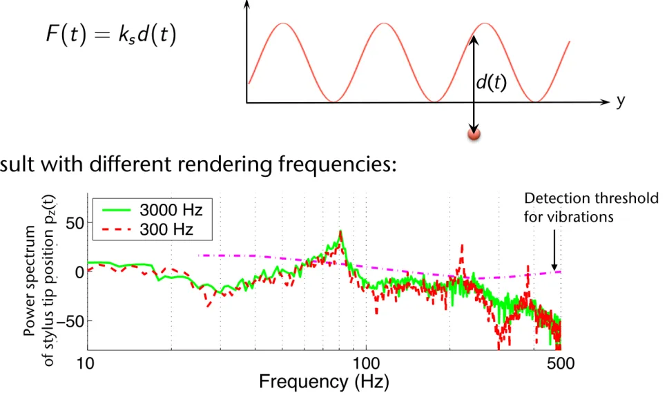
§ The force that is rendered (= output on the actuators):

§ Result with different rendering frequencies:

d(t)

F (t ) = k _s d (t )

10 100 500

10

⁻⁴

10

⁰

Power Spectrum of F z C (t) (N)

10 100 500

10

⁻⁴

10

⁰

Frequency (Hz) Power Spectrum of F z C (t) (N)

Ideal

3000 Hz 300 Hz

Fig. 7. Power spectral densities of the three force commands shown in Fig. 6.

10 100 500

−50 0 50

|P z (f)| (dB re 1 µ m peak)

10 100 500

−50 0 50

Frequency (Hz)

|P z (f)| (dB re 1 µ m peak)

Ideal

3000 Hz 300 Hz

Human Detection Thresholds

Fig. 8. Power spectral densities of the position outputs of the PHANToM along the z-axis (signal C in Fig. 4).

also exhibit significant spectral peaks at 220 and 380 Hz.

Finally, we calculated the output of the Haptic Interface, i.e., the input to the User (signal C in Fig. 4). We assumed that the PHANToM stylus moved around the origin of the PHANToM coordinate frame. We then approximated the dynamics of the PHANToM to the linearized frequency response whose magnitude response was shown earlier in Fig. 3. By multiplying this magnitude response with the power spectral densities of the force commands shown in Fig. 7, we obtained the spectral densities of the PHANToM position outputs.

The results are shown in Fig. 8 along with the hu- man detection thresholds. In the upper panel showing the PHANToM position signal from the ideal force command, only one spectral peak at 80 Hz is well above the human detection threshold. Therefore, we predict that the user will perceive a “clean” texture from the vibration at 80 Hz. In the lower panel, the same can be said about the position signal generated from the force command updated with the ZOH at 3000 Hz. Note, however, that the position signal driven by the force command updated at 300 Hz contains an additional peak at 220 Hz that is well above

the corresponding human detection threshold. We therefore conclude that when forces are updated at 300 Hz, the user will perceive not only the texture information from the vibration at 80 Hz, but also the perceived instability of buzzing from the vibration at 220 Hz. The buzzing noise is subsequently fed back to the Haptic Renderer (through the path D-E-F in Fig. 4). This closed-loop behavior usually increases the intensity of buzzing and widens its frequency range, thereby creating the closed-loop response similar to that shown earlier in Fig. 2.

In summary, the simulation results suggest that using a higher haptic update rate decreases the high-frequency signal content of the reconstructed force command to the force-feedback haptic interface, and consequently reduces the energy of the signal components that can cause the perception of buzzing. A relatively high haptic update rate can be particularly advantageous to force-feedback devices with structural resonances, such as the PHANToM.

V. E XPERIMENT

To verify the simulation results, we conducted a psy- chophysical experiment. The results confirmed that a higher haptic update rate could improve the perceived quality of virtual haptic textures. This section reports the design and results of the psychophysical experiment.

A. Methods

The PHANToM 1.0A model was used to render vir- tual haptic textures. The texture was modeled as one- dimensional sinusoidal gratings (Eq. 1). In all experimental conditions, the amplitude and spatial wavelength of the sinusoidal grating were set to 1 mm and 2 mm, respectively.

The texture model was rendered using F _vec (t) (Eq. 4).

Compared to those rendered with F _mag (t), virtual textures rendered with F _vec (t) exhibit buzzing more often and more intensely. The independent variable in the experiment was the haptic update rate for texture rendering. Eight update rates were tested: 250, 500, 1k, 2k, 5k, 10k, 20k, and 40 kHz. The dependent variable measured in each experi- mental condition was the maximum stiffness threshold K _T under which the textured surface was perceived to be stable without buzzing.

The method of limits, a well-established classical psy- chophysical method [13], was employed to estimate stiff- ness thresholds. The detailed procedure was essentially the same as that used in our previous experiments [1]–

[3]. Each experimental condition consisted of 25 ascending series and 25 descending series. The minimum stiffness (K _min ) and maximum stiffness (K _max ) were set to 0.0 and 1.6 N/mm, respectively, based on preliminary testing.

The increment of stiffness ∆K was 0.05 N/mm for all conditions. More details can be found in [2].

Two subjects (one male and one female) participated in the psychophysical experiment. Both subjects had partici- pated in our previous experiments [1]–[3]. Subject S1 was an experienced user of the PHANToM device. Subject S2 had not used any haptic interface prior to her participation in our previous experiments. The subjects are right-handed

Po w er s p ec tr um of s ty lu s tip p os iti on p

z

(t ) Detection threshold for vibrations

z

y

(28)

Latency in Haptic Feedback

§ General results [2009]:

§ Latency for haptic feedback < 30 msec ⟶ perceived as instantaneous

§ Latency > 30 msec ⟶ subjective user satisfaction drops

§ Latency > 100 msec ⟶ task performance drops

§ Real-life story: touch panel of the info- tainment system of a Cadillac, 2012

§ Conditions: infotainment and tablet, both with touch screen and

haptic feedback, but different delay

Haptic delay

Car Tablet Car Tablet

Feedback magnitude

Delay / msec Magnitude / g

0.7 1.8

28 102

Average rating

Easy to

use Pleasant

to use Felt

confident Was

responsive Knew it received

touch

Felt like real buttons

Car Tablet

Infotainment system in car with haptic touch screen

(29)

Intermediate Representations

§ Problem:

§ Update rate should be 1000 Hz!

§ Collision detection between tip of stylus und virtual environment takes (often) longer than1 msec

§ The VR system needs even more time for other tasks (e.g., rendering, etc.)

§ Solution:

§ Use "intermediate representation" for the current obstacle (typically planes or

spheres)

§ Put haptic rendering in a separate thread

§ Occasionally, send an update of the intermediate representation from the main loop to the haptic thread

constant controls the tightness of the coupling between application and probe; a weaker spring produces small forces in the application while a tighter spring causes more discontinuity in the force when the application endpoint moves.

In order to prevent the user from moving the probe too rapidly, we may in the future add adjustable viscosity to the force-server loop. Viscosity would tend to keep the probe from moving large distances (and thus adding large forces) between simulation time steps.

Multiple springs

Using a single point of contact between the application and the force server, it is only possible to specify forces, not torques. This restriction i s overcome by attaching springs t o multiple application points and multiple virtual probes. Acting together, multiple springs can specify a force and general torque on the probe and the application model (see Figure 5).

2.2 Preventing force discontinuity artifacts As pointed out in [1], the plane-and-probe model works well only when the plane equation is updated frequently compared t o the lateral speed of probe motion. As shown in Figure 6, this restriction is most severe on sharply-curving surfaces. A sharp discontinuity occurs in the force model when the probe i s allowed to move large distances before the new surface approximation is computed. If the discontinuity leaves the probe outside the surface, the probe drops suddenly onto the new level. Worse, if the probe is embedded in the new surface, it is violently accelerated until it leaves the surface (and sometimes the user’s hand).

a b

Figure 6: Probe motion that is rapid compared to the surface curvature causes a sharp discontinuity when the new plane equation arrives. Case a shows the free-fall that occurs for convex surfaces. The more severe case b shows the sudden force caused by being deeply embedded in the surface.

To solve the problem of extreme forces when the probe i s embedded in the new surface, we have developed a recovery time method. This method is applied during the time immediately after new surface parameters arrive. If the probe is outside the surface at the time the parameters change, the system works as described above, dropping suddenly to the surface. If the probe is within the surface, then the normal direction for the force remains as above but the force magnitude is reduced so as t o bring the tip out of the surface over a period of time, rather than instantaneously. This period of time is adjustable, and serves to move the probe out of the surface gently, while still maintaining proper direction for the force at all times. Figure 7 illustrates this algorithm.

n=4

Figure 7: When a new plane equation would cause the probe to be embedded in the surface, the recovery time algorithm artificially lowers the plane to the probe position then raises it linearly to the correct position over n force loop cycles.

This method allows the presentation of much stiffer- feeling surfaces (higher spring constant) without noticeable discontinuities. By using recovery times of up to 0.05 second, the Nanomanipulator application was able to increase the surface spring constant by a factor of 10.

A recovery-time algorithm is also required in the point-to- point spring model. When the only adjustable parameter is the spring constant, there is a trade-off between how tightly the probe is tied to the application endpoint (higher k is better) and how smooth the transition is when the application moves its endpoint (lower k is better). We avoid this tradeoff b y allowing the application to specify the rate of motion for its endpoint after an endpoint update. When the application sets a new position for its endpoint (or a new rest length for the spring), the point smoothly moves from its current location t o the new location over the specified number of server loop iterations.

2.3 Flexibility and extensibility

Our force-feedback software has evolved from application- specific device-driver routines [4], through a device-specific but application-independent library controlling our Argonne- III Remote Manipulator, to the current device-independent remote-access library, Armlib.

Armlib provides connectivity to widely-used graphics engines (SGI, HP and Sun workstations) over commonly-used networks (Ethernet and other TCP/IP). It supports commercially-available force displays (several varieties of SensAble Devices PHANToM [14], and Sarcos Research Corporation Dexterous Master), as well as our Argonne-III Remote Manipulator from Argonne National Laboratories.

Armlib supports the simultaneous use of multiple force- feedback devices, for multi-user or multi-hand applications.

The application selects the device(s) it needs to use at runtime.

Armlib structure

Armlib provides device independence at the API level b y using a cartesian coordinate system with an origin at the center of the device’s working volume. Forces and positions can be automatically scaled so that software will work unchanged with devices of different sizes.

The device independence extends to Armlib’s internal structure (Figure 8). Device-dependencies are compart- mentalized in a set of simple low-level “device-driver”

routines, which handle the reading of joint positions, the writing of joint forces, and the serializing of the robot link configuration. Higher levels of the library, including the intermediate representation servo loops, function in cartesian space. The conversion from joint space to cartesian space and back is handled by a common set of routines which utilize a Denavit-Hartenberg based description of each device t o compute the forward kinematics and Jacobian matrix at runtime (see e.g. [9]). These routines effectively discard most torque Figure 5: Torque

from multiple springs.

450 constant controls the tightness of the coupling between

application and probe; a weaker spring produces small forces in the application while a tighter spring causes more discontinuity in the force when the application endpoint moves.

In order to prevent the user from moving the probe too rapidly, we may in the future add adjustable viscosity to the force-server loop. Viscosity would tend to keep the probe from moving large distances (and thus adding large forces) between simulation time steps.

Multiple springs

Using a single point of contact between the application and the force server, it is only possible to specify forces, not torques. This restriction i s overcome by attaching springs t o multiple application points and multiple virtual probes. Acting together, multiple springs can specify a force and general torque on the probe and the application model (see Figure 5).

2.2 Preventing force discontinuity artifacts As pointed out in [1], the plane-and-probe model works well only when the plane equation is updated frequently compared t o the lateral speed of probe motion. As shown in Figure 6, this restriction is most severe on sharply-curving surfaces. A sharp discontinuity occurs in the force model when the probe i s allowed to move large distances before the new surface approximation is computed. If the discontinuity leaves the probe outside the surface, the probe drops suddenly onto the new level. Worse, if the probe is embedded in the new surface, it is violently accelerated until it leaves the surface (and sometimes the user’s hand).

a b

Figure 6: Probe motion that is rapid compared to the surface curvature causes a sharp discontinuity when the new plane equation arrives. Case a shows the free-fall that occurs for convex surfaces. The more severe case b shows the sudden force caused by being deeply embedded in the surface.

To solve the problem of extreme forces when the probe i s embedded in the new surface, we have developed a recovery time method. This method is applied during the time immediately after new surface parameters arrive. If the probe is outside the surface at the time the parameters change, the system works as described above, dropping suddenly to the surface. If the probe is within the surface, then the normal direction for the force remains as above but the force magnitude is reduced so as t o bring the tip out of the surface over a period of time, rather than instantaneously. This period of time is adjustable, and serves to move the probe out of the surface gently, while still maintaining proper direction for the force at all times. Figure 7 illustrates this algorithm.

n=4

Figure 7: When a new plane equation would cause the probe to be embedded in the surface, the recovery time algorithm artificially lowers the plane to the probe position then raises it linearly to the correct position over n force loop cycles.

This method allows the presentation of much stiffer- feeling surfaces (higher spring constant) without noticeable discontinuities. By using recovery times of up to 0.05 second, the Nanomanipulator application was able to increase the surface spring constant by a factor of 10.

A recovery-time algorithm is also required in the point-to- point spring model. When the only adjustable parameter is the spring constant, there is a trade-off between how tightly the probe is tied to the application endpoint (higher k is better) and how smooth the transition is when the application moves its endpoint (lower k is better). We avoid this tradeoff b y allowing the application to specify the rate of motion for its endpoint after an endpoint update. When the application sets a new position for its endpoint (or a new rest length for the spring), the point smoothly moves from its current location t o the new location over the specified number of server loop iterations.

2.3 Flexibility and extensibility

Our force-feedback software has evolved from application- specific device-driver routines [4], through a device-specific but application-independent library controlling our Argonne- III Remote Manipulator, to the current device-independent remote-access library, Armlib.

Armlib provides connectivity to widely-used graphics engines (SGI, HP and Sun workstations) over commonly-used networks (Ethernet and other TCP/IP). It supports commercially-available force displays (several varieties of SensAble Devices PHANToM [14], and Sarcos Research Corporation Dexterous Master), as well as our Argonne-III Remote Manipulator from Argonne National Laboratories.

Armlib supports the simultaneous use of multiple force- feedback devices, for multi-user or multi-hand applications.

The application selects the device(s) it needs to use at runtime.

Armlib structure

Armlib provides device independence at the API level b y using a cartesian coordinate system with an origin at the center of the device’s working volume. Forces and positions can be automatically scaled so that software will work unchanged with devices of different sizes.

The device independence extends to Armlib’s internal structure (Figure 8). Device-dependencies are compart- mentalized in a set of simple low-level “device-driver”

routines, which handle the reading of joint positions, the writing of joint forces, and the serializing of the robot link configuration. Higher levels of the library, including the intermediate representation servo loops, function in cartesian space. The conversion from joint space to cartesian space and back is handled by a common set of routines which utilize a Denavit-Hartenberg based description of each device t o compute the forward kinematics and Jacobian matrix at runtime (see e.g. [9]). These routines effectively discard most torque Figure 5: Torque

from multiple springs.

length, respectively (see Figure 2). Sinusoidal gratings have been widely used as the basic building blocks for textured surfaces for studies on haptic texture perception (Lederman et al., 1999; Weisenberger et al., 2000).

They have also been used as the basis of a function set for modeling real haptic textures (Wall & Harwin, 1999).

2.2 Texture Rendering Method Two basic texture rendering methods were employed in the current study. Both methods use a spring

model to calculate the magnitude of the rendered force asK!d(t), whereKis the stiffness of the textured surface, andd(t) is the penetration depth of the stylus at timet(see Figure 2). The penetration depth is calculated as follows:

d!t"!

!

Asin!2#px!t/L""⁰ $A% pz!t" ^ifif^pp^zz^!t"!t"^"&⁰0 , (1) where p(t)# (p_x(t),p_y(t),p_z(t)) is the position of the tip of the stylus.

The two methods differ in the way the force directions are rendered. Thefirst method, introduced by Massie (1996), renders a forceF_mag(t) with a constant direction normal to the underlyingflat wall of the textured surface. The second method, proposed by Ho et al. (1999), renders a forceF_vec(t) with varying directions such that it remains normal to the local microgeometry of the sinusoidal texture model. Mathematically,

Fmag!t"!Kd!t"nW, (2)

Fvec!t"!Kd!t"nT!p!t"", (3)

wheren_Wis the normal vector of the underlyingflat wall, andn_T(p(t)) is the normal vector of the textured surface atp(t). Both methods keep the force vectors in the horizontal plane (zxplane in Figure 1), thereby eliminating the effect of gravity on rendered forces.

The two texture rendering methods are natural exten- sions of virtualflat wall rendering techniques. Perceptu- ally, they are very different: textures rendered byF_vec(t) feel rougher than those rendered byF_mag(t) with the same texture model. Textures rendered byF_vec(t) can also feel sticky sometimes.

2.3 Exploration Mode

An exploration mode refers to a stereotypical pattern of the motions that humans employ to perceive a certain object attribute through haptic interaction (Le- derman & Klatzky, 1987). In our experiments, we tested two exploration modes, free exploration and stroking, to examine the effect of user interaction patterns on instability perception. In the free exploration mode, subjects were allowed to use the interaction pattern that Figure 1. An illustration of the virtual textured surfaces and the two

coordinate frames used in our experiments. Position of the stylus tip was always measured in the world coordinate frame.

Figure 2. An illustration of the parameters used in texture rendering.

398 PRESENCE: VOLUME 13, NUMBER 4

(30)

Software Archtecture

§ A haptic device consists of:

§ Sensor measures force (admittance-based) or position (impedance-based)

§ Actuator moves to a specific position (admittance-based) or produces a force/acceleration (impedance-based)

• Archtiecture:

Haptic device Synch.

Collision detection

Interm. Repr.

Position

Position Interm. Repr.

Device driver

Haptic thread

>=1000 Hz Haptic module

>>60 Hz VR System

~ 30 Hz

Force

Position

(31)

Two Principles for Haptic Rendering

§ Dynamic object = object that is being grasped/moved by user;

the end-effector of the haptic device is coupled with the dynamic object

§ Dynamic models:

§ Impedance approach:

haptic device returns current position,

simulation sends new forces to device (to be exerted on human)

§ Admittance approach:

haptic device returns current forces (created by human), simulation accumulates them (e.g. by Euler integration), and sends new positions to device that it assumes directly

§ In both cases, simulation checks collisions between dynamic object and rest of the VE

§ Penalty-based approach: the output force depends on the penetration depth of the dynamic object

§ Requirements:

§ 1000 Hz

§ Constant update rate

(32)