Virtual Reality & Physically-Based Simulation

Virtual Reality &

Physically-Based Simulation

Mass-Spring-Systems

G. Zachmann

University of Bremen, Germany

cgvr.cs.uni-bremen.de

§

Definition:

A mass-spring system is a system consisting of:

1. A set of point masses m_i with positions x_i and velocities v_i, i = 1…n ; 2. A set of springs , where s_ij connects

masses i and j, with rest length l₀ , spring constant k_s (= stiffness) and the damping coefficient k_d

§

Advantages:

§ Very easy to program

§ Ideally suited to study different kinds of solving methods

§ Ubiquitous in games (cloths, capes, sometimes also for deformable objects)

§

Disadvantages:

§ Some parameters (in particular the spring constants) are not obvious, i.e., difficult to derive

§ No built-in volumetric effects (e.g., preservation of volume)

G. Zachmann Virtual Reality & Simulation WS 17 January 2018 Mass-Spring-Systems 6

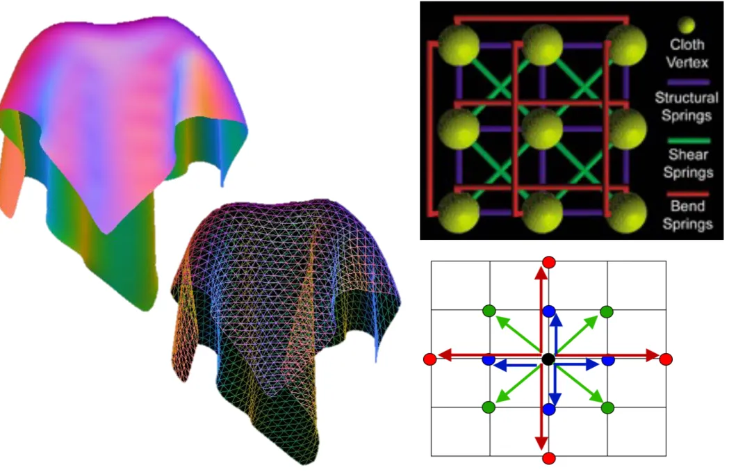
Example Mass-Spring System: Cloth

2 Anonymous

virtually coupled shell system; (2) our model is able to handle complex structures that has loops and branches;

(3) combined with a iterative position-based integra- tor our method allows for a very stable and practical solution; (4) the nature of our framework means it is highly suited to massively parallel execution environ- ments, such as, the GPU; (5) we require no o↵-line pre- processing and the deformations are smooth even for coarse meshes.

2 Related Work

Soft-body systems is a popular multi-discipline topic (e.g., graphics, robotics, animation [20], and medical [5]). Many methods and models have been proposed to simulate deformable bodies, such as, (1) implicit sur- faces [7], (2) finite di↵erence approaches [23], (2) mass- spring systems [9,1], (3) the Boundary Element Method (BEM) [13], (4) the Finite Element Method (FEM) [18,17,6], (5) the Finite Volume Method (FVM) [22], (6) mesh-free particle systems [20,25,8]. While specific methods target accurate scientific/engineering simula- tions, we focus on provide visually plausible emulations.

For example, the finite element method (FEM) targets accurate representations of the stress/decomposition of a model compared to more approximate systems, such as, a mass-spring method.

The inspiring work by Grinspun et al. [11], presented a single outer membrane method which connected the surface using distance constraints for the edges in con- junction with angular constraints for the faces to syn- thesize a soft-body mesh. Our method uses only dis- tance constraints and attempts to account for the sur- faces finite thickness by adding ‘virtual’ shells to add structural support (see Figure 3).

3 Method

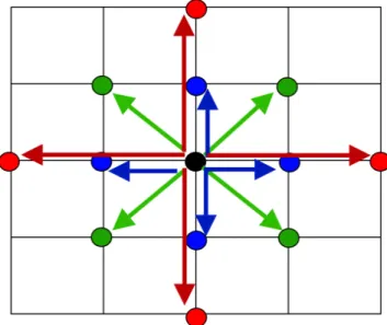
Our approach builds upon a popular penalty-based cloth- spring simulation concept. We use a set of intercon- nected point-masses to represent the physical shape of the mesh. A planar mesh surface is connected using three types of spring, i.e., a bend, a structural, and a shear spring, to synthesize an aesthetically pleasing e↵ect (i.e., smooth responsive deformations). The in- ternal forces from the springs in combination with the topological configuration provide an interactive solu- tion that is able to react to external forces, like gravity and collisions, in a realistic manner.

Fig. 3 Thin Surfaces Concept - Illustrating the problem this paper addresses and solves. (a) a thin surface can be con- nected by any number of distance constraints, however, due to the constraints being parallel, the surface will be unable to keep its rigidity; (b) simple example of a flat surface attached to a wall, the surface will bend under the influence of grav- ity; (c) Grinspun et al. [11] presented a solution to rectify the problem by adding angular springs to neighbouring faces; (d) our approach solves the problem by adding ‘virtual’ parallel layers to the surface that can be connected to provide rigidity to the mesh so it can support itself.

Fig. 4 Point-Mass Coupling - Spatial coupling of neigh- bouring constraints along the surface axis, which we can also apply to the vertically projected shells.

3.1 Dynamics

We define general constraints via a constraint function ([24,19,1]). Instead of computing forces as the deriva- tive of a constraint function energy, we directly solve for the equilibrium configuration and project positions.

With our method we derive a bending term for the ma- terial which uses a point based approach similar to the one proposed by Grinspun et al. [11] and Bridson et al.

[3].

Position-based dynamics have been used for a va- riety of systems. For example, Jakobsen [12] built his physics engine (called Fysix) on a position-based ap- proach. With the central idea of using a Verlet inte- grator to manipulate positions directly. The velocities are implicitly stored by the current and the previous

A Single Spring (Plus Damper)

§

Given: masses m_i and m_j with positions x_i , x_j

§

Let

§

The force between particles i and j :

1. Force exerted by spring (Hooke's law):

acts on particle i in the direction of j

2. Force exerted on i by damper:

3. Total force on i : 4. Force on m_j :

i j

r_ij

-f^ij

l

0

f^ij

k_s

k_d

m_i m_j

r

_ij

= x

_j

x

_i

⇥ x

_j

x

_i

⇥

f

_s^ij

= k

_s

r

_ij

( k x

_j

x

_i

k l

₀

)

f

_d^ij

= k

_d

((v

_i

v

_j

) · r

_ij

)r

_ij

§

A spring-damper element in reality:

§

Alternative spring force:

§

Notice: from (4) it follows that the total momentum is conserved

§ Momentum p = v^.m

§ Fundamental physical law (follows from Newton's laws)

§

Note on terminology:

§ English "momentum" = German "Impuls" = velocity × mass

§ English "Impulse" = German "Kraftstoß" = force × time

Remarks

f_s^{i j} = k_sr_{i j} kx_j x_ik l₀ l₀

Simulation of a Single Spring

§

From Newton’s law, we have:

§

Convert differential equation (ODE) of order 2 into ODE of order 1:

§

Initial values (boundary values):

§

"Simulation" = "Integration of ODE's over time"

§

By Taylor expansion we get:

§

Analogously:

à This integration scheme is called explicit Euler integration

x(t + t ) = x(t ) + t ˙x(t ) + O t

²

⇥

¨x =

_m¹

f

v(t

₀

) = v

₀

, x(t

₀

) = x

₀

˙x(t ) = v(t )

˙v(t ) =

_m¹

f (t )

The Algorithm for a Mass-Spring System

forall particles i : initialize x_i, v_i, m_i

loop forever:

forall particles i :

forall particles i :

render the system every n-th time

f ^g = gravitational force

f ^coll = penalty force exerted by collision (e.g., from obstacles)

f

_i

f

^g

+ f

_i^coll

+

j, (i,j) S

f (x

_i

, v

_i

, x

_j

, v

_j

)

v

_i

+ = t · f

_i

m

i

x

_i

+ = t · v

_i

§

Advantages:

§ Can be implemented very easily

§ Fast execution per time step

§ Is "trivial" to parallelize on the GPU (⟶ "Massively Parallel Algorithms")

§

Disadvantages:

§ Stable only for very small time steps

- Typically Δt ≈ 10^-4 … 10^-3 sec!

§ With large time steps, additional energy is generated "out of thin air", until the system explodes J

§ Example: overshooting when simulating a single spring

§ Errors accumulate quickly

Example for the Instability of Euler Integration

§

Consider the differential equation

§

The exact solution:

§

Euler integration does this:

§

Case :

⇒ x^t oscillates about 0, but approaches 0 (hopefully)

§

Case : ⇒ x^t → ∞ !

˙x (t ) = kx (t ) x (t ) = x

0

e

^kt

x

^t+1

= x

^t

+ t ( kx

^t

) t >

_k¹

x

^t+1

= x

^t

(1 k t )

⇤ ⇥ ⌅

<0

t >

_k²

§

Visualization:

§

Terminology: if k is large → the ODE is called "stiff "

§ The stiffer the ODE, the smaller Δt has to be

time

position

˙x (t ) = x (t )

Visualization of Error Accumulation

§

Consider this ODE:

§

Exact solution:

§

The solution by Euler integration moves in spirals outward, no

matter how small Δt!

§

Conclusion: Euler integration accumulates errors, no matter how small Δt!

x(t ) = r cos(t + ) r sin(t + )

⇥

˙x(t ) =

✓ –x

2

x

1

◆

Visualization of Differential Equations

§

The general form of an ODE (ordinary differential equation):

§

Visualization of f as a vector field:

§ Notice: this vector field can vary over time!

§

Solution of a boundary value problem = path through this field

˙x(t ) = f ( x(t ), t )

Other Integrators

§

Runge-Kutta of order 2:

§ Idea: approximate f( x(t), t ) by using the derivative at positions x(t) and x( t+ ½Δt )

§ The integrator (w/o proof):

§

Runge-Kutta of order 4:

§ The standard integrator among the explicit integration schemata

§ Needs 4 function evaluations (i.e., force computations) per time step

§ Order of convergence is:

e ( t ) = O t

⁴

⇥

a

₁

= v

^t

a

₂

= 1

m f (x

^t

, v

^t

) b

₁

= v

^t

+ 1

2 t a

₂

b

₂

= 1

m f x

^t

+ 1

2 t a

₁

, v

^t

+ 1

2 t a

₂

x

^t+1

= x

^t

+ t b

₁

v

^t+1

= v

^t

+ t b

₂

§

Runge-Kutta of order 2:

§

Runge-Kutta of order 4:

Euler

Verlet Integration

§

A general, alternative idea to increase the order of convergence:

utilize values from the past

§

Verlet integration = utilize x( t - Δt )

§

Derivation:

§ Develop the Taylor series in both time directions:

x(t + t ) = x(t ) + t ˙x(t ) + 1

2 t

²

¨ x(t ) + 1

6 t

³

...

x (t ) + O t

⁴

⇥

x(t t ) = x(t ) t ˙x(t ) + 1

2 t

²

¨ x(t ) 1

6 t

³

...

x (t ) + O t

⁴

⇥

§ Add both:

§

Initialization:

§

Remark: the velocity does not occur any more!

(at least, not explicitly)

x( t ) = x(0) + t v(0) + 1

2 t

²

1

m f (x(0), v(0)) ⇥

Constraints

§

Big advantage of Verlet over Euler & Runge-Kutta:

it is very easy to handle constraints

§

Definition: constraint = some condition on the position of one or more mass points

§

Examples:

1. A point must not penetrate an obstacle

2. The distance between two points must be constant, or distance must be ≤ some maximal distance

§

Example: consider the constraint

1. Perform one Verlet integration step → 2. Enforce the constraint:

§

Problem: if several constraints are to constrain the same mass point, we need to employ constraint satisfaction algorithms

d d

⇥ x

₁

x

₂

⇥ =

^!

l

₀

x₁ l₀ x₂

~ ~

d = 1

2 ( || ˜ x

^t₂⁺¹

˜ x

^t+1₁

|| l

0

) x

^t₁⁺¹

= ˜ x

^t₁⁺¹

+ d r

₁₂

x

^t₂⁺¹

= ˜ x

^t₂⁺¹

d r

₁₂

Time-Corrected Verlet Integration

§

Big assumption in basic Verlet: time-delta's are constant!

§

Solution for non-constant Δ_t's:

§ Time steps are: and

§ Expand Taylor series in both directions:

and

§ Divide the expansions by and , respectively, then add both, like in the derivation of the basic Verlet

§ Rearranging and omitting higher-order terms yields:

§

Note: basic Verlet is a special case of time-corrected Verlet

x(t

_i

+ t

_i

)

t

_i+1

= t

_i

+ t

_i

t

_i

= t

_{i 1}

+ t

_{i 1}

x(t

_i

t

_{i 1}

)

x(t_i + t_i) = x(t_i) + t_i

t_{i 1} x(t_i) x(t_i t_{i 1}) + ¨x(t_i) t_i + t_{i 1}

2 · t_i

t

_i

t

_{i 1}

Implicit Integration (a.k.a. Backwards Euler)

§

All explicit integration schemes are only conditionally stable

§ I.e.: they are only stable for a specific range for Δt

§ This range depends on the stiffness of the springs

§

Goal: unconditionally stability

§

One option: implicit Euler integration

§

Now we've got a system of non-linear, algebraic equations, with x^t+1 and v^t+1 as unknowns on both sides → implicit integration

x

^t_i⁺¹

= x

^t_i

+ t v

^t_i

x

^t_i⁺¹

= x

^t_i

+ t v

^t_i⁺¹

explicit implicit

v

^t_i⁺¹

= v

^t_i

+ t 1

m

_i

f (x

^t+1

) v

_i^t+1

= v

^t_i

+ t 1

m

_i

f (x

^t

)

Solution Method

§

Write the whole spring-mass system with vectors (n = #mass points):

x = 0 BB B@

x₀ x₁ ...

x_{n 1} 1 CC CA =

0 BB BB BB B@

x₀ x₁ x₂ x₃ ...

x_{3n 1} 1 CC CC CC CA

, v =

0 BB B@

v₀ v₁ ...

v_{n 1} 1 CC CA =

0 BB BB BB B@

v₀ v₁ v₂ v₃ ...

v_{3n 1} 1 CC CC CC CA

, f(x) =

0 B@

f₀(x) ...

f_{n 1}(x) 1 CA

fi = 0

@f3i+0(x) f_3i+1(x) f_3i+2(x)

1

A , M3n x3n = 0 BB BB BB BB BB BB B@

m0

m₀

m₀

m1

m1

. ..

mn 1

m_{n 1}

m_{n 1} 1 CC CC CC CC CC CC CA

§

Write all the implicit equations as one big system of equations :

§

Plug (2) into (1) :

§

Expand f as Taylor series:

M v

^t+1

= M v

^t

+ t f (x

^t+1

) (1)

x

^t+1

= x

^t

+ t v

^t+1

(2)

M v

^t+1

= M v

^t

+ t f ( x

^t

+ t v

^t+1

)

⁽³⁾

(4)

§

Plug (4) into (3):

§

K is the Jacobi-Matrix, i.e., the derivative of f wrt. x:

§ K is called the tangent stiffness matrix

- (The normal stiffness matrix is evaluated at the equilibrium of the system:

here, the matrix is evaluated at an arbitrary "position" of the system in phase space, hence the name "tangent …")

M v

^t+1

= M v

^t

+ t ⇣

f (x

^t

) + @

@ x f (x

^t

)

| {z }

K

· t v

^t+1

⌘

= M v

^t

+ t f (x

^t

) + t

²

K v

^t+1

K =

0 B @

@

@x₀

f

_{0 @x}^@

1

f

₀

. . .

_@x^@

3n 1

f

₀

... ... . .. ...

@

@x₀

f

_{3n 1}

. . . . . .

_@x^@

3n 1

f

_{3n 1}

1

C A

§

Reorder terms :

§

Now, this has the form:

§

Solve this system of linear equations with any of the standard iterative solvers

§

Don't use a non-iterative solver, because

§ A changes with every simulation step

§ We can "warm start" the iterative solver with the solution as of last frame

- Incremental computation

Computation of the Stiffness Matrix

§

First, understand the anatomy of matrix K :

§ A spring (i , j) adds the following four 3x3 block matrices to K :

§ Matrix K_ij arises from the derivation of f_i = (f_3i,f_3i+1, f_3i+2) wrt. x_j= (x_3j,x_3j+1, x_3j+2):

§ In the following, consider only f^s (spring force) 3i

3j

3i 3j

i j

K

_ij

= 0 B @

@

@x_3j

f

_{3i @x}^@

3j+1

f

_{3i @x}^@

3j+2

f

_3i

... ...

@

@x_3j

f

_3i+2

· · ·

_@x3j^@₊₂

f

_3i+2

1

C A

§ First of all, compute K_ii:

K

_ii

= @

@x

_i

f

_i

(x

_i

, x

_j

)

= k

_s

@

@ x

_i

⇣ (x

_j

x

_i

) l

₀

x

_j

x

_i

k x

_j

x

_i

k

⌘

= k

_s

0

@ I l

₀

I · k x

_j

x

_i

k (x

_j

x

_i

) ·

^(x_kx^j_j ^x_xⁱ⁾_ik^>

k x

_j

x

_i

k

²

1 A

= k

s

✓

I + l

0

1

k x

j

x

i

k I + l

0

k x

j

x

i

k

³

(x

j

x

i

)(x

j

x

i

)

^T

◆

§

Reminder:

§

§

@

@x k x k = @

@x

✓q

x

₁²

+ x

₂²

+ x

₃²

◆

= x

^T

k x k

§

From some symmetries, we can analogously derive:

§

§

§

K

_ij

=

x

_j

f

_i

(x

_i

, x

_j

) = K

_ii

K

_jj

=

x

_j

f

_j

(x

_i

, x

_j

) =

x

_j

( f

_i

(x

_i

, x

_j

)) = K

_ii

Overall Algorithm for Solving Implicit Euler Integration

§

Initialize K = 0

§

For each spring (i , j) compute K_ii, K_ij, K_ji, K_jj and accumulate it to K at the right places

§

Compute

§

Solve the linear equation system →

§

Compute

x

^t+1

= x

^t

+ t v

^t+1

Av

^t+1

= b

b = M v

^t

+ t f (x

^t

)

Advantages and Disadvantages

§

Explicit integration:

+ Very easy to implement - Small step sizes needed

- Stiff springs don't work very well

- Forces are propagated only by one spring per time step

§

Implicit Integration:

+ Unconditionally stable + Stiff springs work better

+ Global solver → forces are being propagated throughout the whole spring-mass system within one time step

- Large stime steps are needed, because one step is much more expensive (if real-time is needed)

- The integration scheme introduces damping by itself (might be unwanted)

§

Visualization of:

§

Informal Description:

§ Explicit jumps forward blindly, based on current information

§ Implicit tries to find a future position and a backwards jump such that the backwards jump arrives exactly at the current point (in phase space)

time

position

˙x (t ) = x (t )

Demo

G. Zachmann Virtual Reality & Simulation WS 17 January 2018 Mass-Spring-Systems 39

Mesh Creation for Volumetric Objects

§

How to create a mass-spring system for a volumetric model?

§ Challenge: volume preservation!

§

Approach 1: introduce additional, volume-preserving constraints

§ Springs to preserve distances between mass points

§ Springs to prevent shearing

§ Springs to prevent bending

§

No change in model & solver required

§

You could also introduce

"angle-preserving springs" that exert a torque on an edge

2 Anonymous

virtually coupled shell system; (2) our model is able to handle complex structures that has loops and branches;

(3) combined with a iterative position-based integra- tor our method allows for a very stable and practical solution; (4) the nature of our framework means it is highly suited to massively parallel execution environ- ments, such as, the GPU; (5) we require no o↵-line pre- processing and the deformations are smooth even for coarse meshes.

2 Related Work

Soft-body systems is a popular multi-discipline topic (e.g., graphics, robotics, animation [20], and medical [5]). Many methods and models have been proposed to simulate deformable bodies, such as, (1) implicit sur- faces [7], (2) finite di↵erence approaches [23], (2) mass- spring systems [9,1], (3) the Boundary Element Method (BEM) [13], (4) the Finite Element Method (FEM) [18,17,6], (5) the Finite Volume Method (FVM) [22], (6) mesh-free particle systems [20,25,8]. While specific methods target accurate scientific/engineering simula- tions, we focus on provide visually plausible emulations.

For example, the finite element method (FEM) targets accurate representations of the stress/decomposition of a model compared to more approximate systems, such as, a mass-spring method.

The inspiring work by Grinspun et al. [11], presented a single outer membrane method which connected the surface using distance constraints for the edges in con- junction with angular constraints for the faces to syn- thesize a soft-body mesh. Our method uses only dis- tance constraints and attempts to account for the sur- faces finite thickness by adding ‘virtual’ shells to add structural support (see Figure 3).

3 Method

Our approach builds upon a popular penalty-based cloth- spring simulation concept. We use a set of intercon- nected point-masses to represent the physical shape of the mesh. A planar mesh surface is connected using three types of spring, i.e., a bend, a structural, and a shear spring, to synthesize an aesthetically pleasing e↵ect (i.e., smooth responsive deformations). The in- ternal forces from the springs in combination with the topological configuration provide an interactive solu- tion that is able to react to external forces, like gravity and collisions, in a realistic manner.

Fig. 3 Thin Surfaces Concept - Illustrating the problem this paper addresses and solves. (a) a thin surface can be con- nected by any number of distance constraints, however, due to the constraints being parallel, the surface will be unable to keep its rigidity; (b) simple example of a flat surface attached to a wall, the surface will bend under the influence of grav- ity; (c) Grinspun et al. [11] presented a solution to rectify the problem by adding angular springs to neighbouring faces; (d) our approach solves the problem by adding ‘virtual’ parallel layers to the surface that can be connected to provide rigidity to the mesh so it can support itself.

Fig. 4 Point-Mass Coupling - Spatial coupling of neigh- bouring constraints along the surface axis, which we can also apply to the vertically projected shells.

3.1 Dynamics

We define general constraints via a constraint function ([24,19,1]). Instead of computing forces as the deriva- tive of a constraint function energy, we directly solve for the equilibrium configuration and project positions.

With our method we derive a bending term for the ma- terial which uses a point based approach similar to the one proposed by Grinspun et al. [11] and Bridson et al.

[3].

Position-based dynamics have been used for a va- riety of systems. For example, Jakobsen [12] built his physics engine (called Fysix) on a position-based ap- proach. With the central idea of using a Verlet inte- grator to manipulate positions directly. The velocities are implicitly stored by the current and the previous

§

Approach 2 (and still simple): model the inside volume explicitly

§ Create a tetrahedron mesh out of the geometry (somehow)

§ Each vertex (node) of the tetrahedron mesh becomes a mass point, each edge a spring

§ Distribute the masses of the tetrahedra (= density × volume) equally among the mass points

§

Generation of the tetrahedron mesh (simple method):

§ Distribute a number of points uniformly (perhaps randomly) in the interior of the geometry (so called "Steiner points")

§ Dito for a sheet/band above the surface

§ Connect the points by Delaunay triangulation (see my course

"Computational Geometry for CG")

§

Anchor the surface mesh within the tetrahedron mesh:

§ Represent each vertex of the surface mesh by the barycentric combination of its surrounding tetrahedron vertices

G. Zachmann Virtual Reality & Simulation WS 17 January 2018 Mass-Spring-Systems 42

§

Approach 3: kind of an "in-between" between approaches 1 & 2

§ Create a virtual shell around the two-manifold mesh

§ Connect the shell with the "real" mesh by diagonal springs

§

Video:

1. no virtual shells, 2. one virtual shell, 3. several virtual shells

2 Anonymous

virtually coupled shell system; (2) our model is able to handle complex structures that has loops and branches;

(3) combined with a iterative position-based integra- tor our method allows for a very stable and practical solution; (4) the nature of our framework means it is highly suited to massively parallel execution environ- ments, such as, the GPU; (5) we require no o↵-line pre- processing and the deformations are smooth even for coarse meshes.

2 Related Work

Soft-body systems is a popular multi-discipline topic (e.g., graphics, robotics, animation [20], and medical [5]). Many methods and models have been proposed to simulate deformable bodies, such as, (1) implicit sur- faces [7], (2) finite di↵erence approaches [23], (2) mass- spring systems [9, 1], (3) the Boundary Element Method (BEM) [13], (4) the Finite Element Method (FEM) [18, 17, 6], (5) the Finite Volume Method (FVM) [22], (6) mesh-free particle systems [20, 25, 8]. While specific methods target accurate scientific/engineering simula- tions, we focus on provide visually plausible emulations.

For example, the finite element method (FEM) targets accurate representations of the stress/decomposition of a model compared to more approximate systems, such as, a mass-spring method.

The inspiring work by Grinspun et al. [11], presented a single outer membrane method which connected the surface using distance constraints for the edges in con- junction with angular constraints for the faces to syn- thesize a soft-body mesh. Our method uses only dis- tance constraints and attempts to account for the sur- faces finite thickness by adding ‘virtual’ shells to add structural support (see Figure 3).

3 Method

Our approach builds upon a popular penalty-based cloth- spring simulation concept. We use a set of intercon- nected point-masses to represent the physical shape of the mesh. A planar mesh surface is connected using three types of spring, i.e., a bend, a structural, and a shear spring, to synthesize an aesthetically pleasing e↵ect (i.e., smooth responsive deformations). The in- ternal forces from the springs in combination with the topological configuration provide an interactive solu- tion that is able to react to external forces, like gravity and collisions, in a realistic manner.

Fig. 3 Thin Surfaces Concept - Illustrating the problem this paper addresses and solves. (a) a thin surface can be con- nected by any number of distance constraints, however, due to the constraints being parallel, the surface will be unable to keep its rigidity; (b) simple example of a flat surface attached to a wall, the surface will bend under the influence of grav- ity; (c) Grinspun et al. [11] presented a solution to rectify the problem by adding angular springs to neighbouring faces; (d) our approach solves the problem by adding ‘virtual’ parallel layers to the surface that can be connected to provide rigidity to the mesh so it can support itself.

Fig. 4 Point-Mass Coupling - Spatial coupling of neigh- bouring constraints along the surface axis, which we can also apply to the vertically projected shells.

3.1 Dynamics

We define general constraints via a constraint function ([24, 19, 1]). Instead of computing forces as the deriva- tive of a constraint function energy, we directly solve for the equilibrium configuration and project positions.

With our method we derive a bending term for the ma- terial which uses a point based approach similar to the one proposed by Grinspun et al. [11] and Bridson et al.

[3].

Position-based dynamics have been used for a va-

riety of systems. For example, Jakobsen [12] built his

physics engine (called Fysix) on a position-based ap-

proach. With the central idea of using a Verlet inte-

grator to manipulate positions directly. The velocities

are implicitly stored by the current and the previous

Collision Detection for Mass-Spring Systems

§

Put all tetrahedra in a 3D grid (use a hash table!)

§

In case of a collision in the hash table:

§ Compute exact intersection between the 2 involved tetrahedra

Collision Response

§

Given: objects P and Q (= tetrahedral meshes) that collide

§

Task: compute a penalty force

§

Naïve approach:

§ For each mass point of P that has penetrated, compute its

closest distance from the surface of Q → force = amount + direction

§

Problem:

§ Implausible forces

§ "Tunneling" (s. a. the chapter on force-feedback)

University of Freiburg - Institute of Computer Science - Computer Graphics Laboratory

!

rigid and deformable objects

!

collisions, self-collisions, n-body environments

!

memory efficient, interactive

Spatial Hashing - Summary

Collision Response

University of Freiburg - Institute of Computer Science - Computer Graphics Laboratory

Introduction

!

computation of penalty forces based on the penetration depth of intersecting vertices

University of Freiburg - Institute of Computer Science - Computer Graphics Laboratory

Challenges

!

inconsistent penetration depth information due to discrete simulation steps and object discretization

!

[Heidelberger, Teschner et al. 2003]

inconsistent consistent inconsistent consistent

Q

P

§

Examples:

inconsistent consistent

G. Zachmann Virtual Reality & Simulation WS 17 January 2018 Mass-Spring-Systems 46

Consistent Penalty Forces

1. Phase: identify all points of P that penetrate Q

2. Phase: determine all edges of P that intersect the surface of Q

§ For each such edge, compute the exact intersection point x_i

§ For each intersection point, compute a normal n_i

- E.g., by barycentric interpolation of the vertex normals of Q

P Q

University of Freiburg - Institute of Computer Science - Computer Graphics Laboratory

Algorithm – Stage 1

! object points are classified as colliding or non-colloding points ! spatial hashing

non-colliding point colliding point

University of Freiburg - Institute of Computer Science - Computer Graphics Laboratory

Algorithm – Stage 2

! border points, intersecting edges, and intersection points are detected ! extended spatial hashing

intersection edge border point intersection point intersection normal

University of Freiburg - Institute of Computer Science - Computer Graphics Laboratory

Algorithm – Stage 3

! penetration depth d(p) of a border point p is approximated using the adjacent intersection points x_i and normals n_i

University of Freiburg - Institute of Computer Science - Computer Graphics Laboratory

Algorithm – Stage 4

! consistent penetration depth information at points p_j is propagated to other colliding points p

G. Zachmann Virtual Reality & Simulation WS 17 January 2018 Mass-Spring-Systems 47

3. Phase: compute the approximate force for border points

§ Border point = a point p that penetrates Q and is incident to an intersecting edge

§ Observation: a border point can be incident to several intersecting edges

§ Set the penetration depth for point p to

where d(p) = approx. penetration depth of mass point p, x_i = point of the

intersection of an edge incident to p with surface Q, n_i = normal to surface of Q at point x_i ,

and

d (p) =

k

i=1

(x

_i

, p) (x

_i

p) · n

_i

k

i=1

(x

_i

, p)

(x_i,p) = 1

⇥x_i p⇥

•5

University of Freiburg - Institute of Computer Science - Computer Graphics Laboratory

Algorithm – Stage 1

!

object points are classified as colliding

or non-colloding points ! spatial hashing

non-colliding point colliding point

University of Freiburg - Institute of Computer Science - Computer Graphics Laboratory

Algorithm – Stage 2

!

border points, intersecting edges, and intersection points are detected ! extended spatial hashing

intersection edge border point

intersection point intersection normal

University of Freiburg - Institute of Computer Science - Computer Graphics Laboratory

Algorithm – Stage 3

!

penetration depth d(p) of a border point p is approximated using the adjacent intersection points x _i and normals n _i

University of Freiburg - Institute of Computer Science - Computer Graphics Laboratory

Algorithm – Stage 4

!

consistent penetration depth information at points p _j is propagated to other colliding points p

Q

P

§ Direction of the penalty force on border points:

4. Phase: propagate forces by way of breadth-first traversal through the tetrahedron mesh

where p_i = points of P that have been visited already, p = point not yet visited, r_i = direction of the estimated penalty force in point p_i .

d (p) =

⇤

k

i=1

(p

_i

, p) (p

_i

p) · r

_i

+ d (p

_i

) ⇥

⇤

k

i=1

(x

_i

, p)

r(p) =

P

k

i=1

!(x

_i

, p) n

_i

P

k

i=1

!(x

_i

, p)

Visualization

Video