Error Rates in Multivariate Classication
C. Weihs
Fachbereich Statistik
Universitat Dortmund
G. Calzolari
Dipartimento di Statistica
Universita degli studi di Firenze
M. C. Rohl
Konigstein /Ts.
August 1999
Abstract
Inthispaper,controlvariatesareproposedtospeedupMonteCarloSim-
ulationsto estimateexpected errorratesinmultivariateclassication.
KEY WORDS: classication, control variates, error rate, Monte Carlo
Simulation,variancereduction
1 Introduction
TheaimofthispaperistospeedupMonteCarloSimulationsappliedtomultivariate
classication. The most interesting performance measure in classication is the
misclassicationerror.
In thecase ofgiven groupdensities, thereare two possibilitiestocalculatethe error
rate: eitherbynumericalintegrationorbyMonteCarloSimulationwhichistheonly
feasible method in higher dimensions. In this paper, we focus on the Monte Carlo
errorestimate. This approach suersfromthe variabilityofthe errorrates, because
the error rate is a random variable by now. Therefore, every principle to reduce
this varianceiswelcome. Inthe literaturevariousvariancereduction techniquesare
proposed,amongthoseantitheticvariablesandcontrolvariates(see,e.g., [1]). Here,
D-44221Dortmund,Germany,Tel. ++49-231-755-4363,e-mail: weihs@amadeus.statistik.uni-
dortmund.de
we will concentrate on control variates and demonstrate their variance reduction
potentialin our special problem.
The paper is organized as follows: In section 2 we will give a brief introduction to
multivariateclassication. Insection3,wewillproposetwodierentcontrolvariates
which willbe studied and compared in section 4 by means of some examples. The
papercloses with a conclusion insection 5.
2 Multivariate Classication
Classicationdealswiththeallocationofobjectstog predeterminedgroups1;2;::: ;
g, say. The aim is to minimize the misclassication error (rate) over all possible
future allocations, given the group densities p
i
(x) ( i= 1 ;2;::: ;g). The minimal
error rate is the so{calledBayeserror.
Wemeasure d features(variables)of the objects weconsider importantfordiscrim-
ination between the objects. These can becontinuous features (GNP,consumption
etc.) ordiscrete (number of rms,numberof inhabitants etc.).
Oncethegroupdensitiesarespecied,inordertominimizetheerrorrateweallocate
anobject with feature vector x to groupi, if
p
i
(x)>p
j
(x) ( 6=j i): (1)
Classication methods often assume the group densities p
i
(x) to be normal. Then
there are at least two modellingpossibilities(see, e.g., [2]):
Estimatethe same covariancematrix forall groups(LDA,linear discriminant
analysis) or
estimate a dierent covariance matrix for each group (QDA, quadratic dis-
criminantanalysis).
Ofcourse,bothmethodsalsoestimatedierentmeanvectorsforeachgroup. Inthis
paperwe take QDA asthe adequate, and thus standard classication procedure.
Oftenweadditionallywanttoreducethedimensionfromdtod 0
=1or2toenhance
human perception (dimensionreduction). Theconstruction ofad 0
{spacewith min-
imalerror rate, given the group densities p
i
(x) ind{space, can be done by modern
optimizationtechniques, forexampleSimulatedAnnealing[3]. In eachoptimization
step, aprojection space isproposed. Then wedetermine the groupdensities(either
estimated by means of the projected data or directly derived from the projected
densities of the original space) [4], and calculate the error rate in the projection
space.
Inthis paper,wesuppose thatthe projection spaceisxed, sothat wealreadyhave
the group densitiesavailable. Ofcourse, thefollowingapproach can bealsoapplied
during optimizationat each optimizationstep.
3 Variance Reduction by Control Variates
3.1 General Ideas
What wehave tocalculateistheerrorrate given thegroupdensities. In onedimen-
sion, this can easilybe doneby numericalintegration, becausewe onlyhaveto nd
theintersectionpointsofthedierentgroupdensities(determinedbyp
i
(x)=p
j (x))
and then calculateintegralslike
Z
b
a p
i
(x)dx a;b2R; (2)
where p
i
(x)denotes anarbitrary known group density.
But intwo ormore dimensions, the borderlines between the group densitiesdonot
have that simple shapes, even when we assume equal group covariance matrices.
Therefore, integration can only be done by means of a grid in two or more dimen-
sions.
Another possibility to calculatethe error rate is Monte Carlo Simulation. We gen-
erate random realizations from the group densities and allocate them according to
our classication rule (1). This approach suers from the variability of the error
rates, because the error rate is arandom variable by now.
In order toreduce the Monte Carlo variance of the error rate we introduce control
variates (cv). Theobjectof interestis theerror rateerror. Wewrite this inamore
complicated but helpful way as
error=error
cv
+(error error
cv
) (3)
with a new randomvariable error
cv
. Wewant to compute the expectation of these
error rates
E(error)=E (error
cv
)+E (error error
cv
): (4)
The idea behind controlvariatesis to choose a randomvariableerror
cv
so that we
can calculate E(error
cv
)exactly (no variance)and error and error
cv
are positively
correlated. Soa sensibleway of estimating E(error)would be
^
E
cv
(error)=E(error
cv )+
^
E(error error
cv
); (5)
where the rst term onthe right hand side has novarianceand the second term is
computed as the samplemean of Monte-Carloreplicates. Then the varianceof the
righthand side of (4)is
Var(error error
cv
)=N; (6)
where N is the sample size to determine error and error
cv ,and
Var(error error
cv
)=Var(error)+Var(error
cv )
2Cov (error;error
cv
): (7)
Now it becomes clear that a large positive correlation between error and error
cv
can reduce the variance compared to the "naive" estimator
^
E
MC
(error), i.e. the
sample mean of Monte Carlo replicates of error with variance Var(
^
E
MC
(error))=
Var(error)=N. Wecan even dobetter. Wecan use the equation
E ( error)= E(error
cv
)+E(error error
cv
) (8)
to selectthat parameter that minimizesthe variance
Var(error error
cv
); (9)
leadingto
=
Cov (error;error
cv )
Var(error
cv )
(10)
whichisalmostequaltothecorrelationcoecient%whenVar(error)Var(error
cv )
holds. The nal result is then
min
Var(error error
cv
)(1 % 2
)Var(error); (11)
i.e. there can always bea gain when %6=0.
Considering the above arguments, what we look for as a control variate procedure
is any classicationmethodwhichgivesresults asmuchas possible correlated with
QDA, and for which the exact expected error rate is easilycomputable. Moreover,
one should avoid control variates for which the additional computational eort is
that high that overall computation time is increased even in the case of variance
reduction.
3.2 Two Specic Control Variates
What is, then, a suitablecontrolvariate in our context? We willdiscuss two possi-
bilities. In both cases the control variate procedureassumes a somewhat simplied
problem situation to be true in order to simplify the Monte Carlo procedure. In
the rst procedure the covariance matrices of the dierent groups are assumed to
be identical. In the second procedure the possibly high dimensional problem is
optimally projected to one dimension. Note that we assumed to study problems
with normal group densities with individual covariance matrices. Thus, QDA was
1. The rst idea is to utilize the error rate computed by LDA as error
cv
based
on the assumption of equal covariance matricesfor allthe groups. The error
rate error is calculated by QDA from N random realizations drawn from
the group densities. To get
^
E
MC
(error) we generate W such error rates and
average. Therefore we used N W random vectors. Now we take the same
random vectors and apply LDA with the same, so-called pooled, covariance
matrix for all groups to calculate error rates error
cv
. If
i
is the assumed
covariance matrix for group i, then ( P
g
i=1 (N
i
1)
i
)=(N g) is the pooled
covariance matrix, where N
i
is the number of realizations in group i. The
dierences of the W corresponding estimates error and error
cv
are used to
calculate
^
E(error error
cv
). At last we calculate E (error
cv
) in an exact
manner (so that we have novariance) by numericalintegration based onthe
densitieswithpooled covariancematrices. Wenowhavealltheingredientswe
need for aneciency comparisonwith the naiveMonte Carlo estimator. The
variance of the naive estimator is calculated by the sample of size W of the
estimated error rates error and the variance of the control variate estimator
by thesampleofsize W of(error error
cv
). Thisapproachhas thedrawback
that we have to calculateanexact integral ina projection space whichmight
be two dimensional orof even higher dimension with ratherugly borderlines.
2. A second possibility to determine the error rate error is to use another con-
trol variate: the error rate of an "optimal"one dimensional projection. This
can be obtained by the largest eigenvalue and the corresponding eigenvector
of QDA in the original space or by direct minimization of the error rate. We
do the same as in 1 to obtain
^
E
MC
(error). But then we project the random
vectors onto the optimally discriminating direction taking into account the
dierent covariance structures and build the dierences of corresponding er-
ror estimates to compute
^
E ( error error
cv
). Now, the exact calculation of
E ( error
cv
) is simply a one dimensional integration with clearcut intersection
points. This speeds up the procedure compared to 1. To construct the opti-
mallydiscriminatingonedimensionalprojectionwefollowanideain[5]where
it wasproposed toprojecton the rst eigenvector v
1
of MM T
, where
M =(
g
1
;:::;
2
1
;
g
1
;:::;
2
1
) (12)
wherethe
i
arethe groupmeansand the
i
are (again)the groupcovariance
matrices,i=1,...,g. Theprojectedmeans,variancesandfeaturevectorsthen
havethe form:
i
=v T
1
i ,
i
=v T
1
i v
1
and x
=v T
1 x .
In order torepresent adequate control variates the additionalcomputation time of
procedures1and2havetobesmallrelativetothecomputationtimeofnaiveMonte
Carlo. That this is the case not considering the computation of the exact expected
error rates should be clearby the followingarguments.
Naive Monte Carlo estimates the means and the covariance matrices of the
groups, and evaluates the corresponding estimated group densities for each
Procedure 1additionallyneeds to compute the mean of the estimated covari-
ance matricesofthe groups,and toevaluategroup densitiesfor each observa-
tion corresponding tothe pooled covariance matrix ineach group.
Procedure2additionallycomputesthe'dierencematrix'M,itsrsteigenvec-
tor v
1
, and the corresponding projections of the group means and covariance
matrices, and evaluates the corresponding 1D normal densities in each pro-
jected observation.
Therefore, in procedures 1 and 2 the 'preparation' of the density evaluation does
not depend on the number of observations, resulting in a much smaller additional
'preparationtime'thanthe preparationtimefornaiveMonteCarloforbignumbers
of observations. Moreover, in procedure 2 also the additional density evaluations
are much quickerthan the density evaluationsinnaive MonteCarlo, since they are
in1D.
In procedure 1 the exact expected error rates have to be calculated numerically, in
general. For the exact expected error rates in procedure 2, however, an analytic
formulacan bederived, even. Thiswillbedone inthe next subsection. In section4
we willdemonstrate the dierences between procedures 1 and 2 by some examples.
3.3 Exact expected error rates
Inprocedure2exactexpectederrorrateshavetobecalculatedforunivariatenormal
projected distributions. In this case ageneral formulafor the exact expected error
rate could be given depending on the intersection points of the univariate normal
densities corresponding to the projected group means and variances. In order to
illustratethe idea, letus discuss the 2and 3 groups cases. Moreover, let usassume
equal a-prioriprobabilities 1=g for all g groups for simplicity. In the simulationsin
the followingsections, we alsowilldiscuss these cases only.
In the case of2groups letthe intersection pointof the two normaldensitiesbe x
12 .
Then, obviously, the exact expected error rate corresponding to these densities is
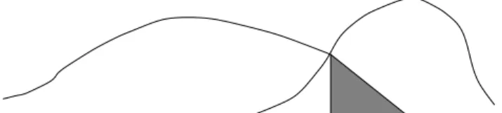
(cp. gure 1)
E(error
cv
)=((1
1 (x
12 )+
2 (x
12
))=2) (13)
where
1
is the normal distributionwith mean tothe left of x
12
, and
2
the distri-
bution with mean tothe right.
In the case of 3 groups let the distribution indices again be chosen so that a lower
index indicates a lower mean. We are now interested in the relative location of
the intersection points of the 3 densities. The error rate of the leftmost group 1 is
determined by the rst intersection onthe righthand side withone of the densities
of the other groups. For the rightmost group 3 the same is true for the densities
Figure 1: The error rate of the leftgroup is gray shaded.
the rst intersections points of its density with the other densities on the left and
onthe right. For simplicitylet usnow assume that the relevant intersection points
are x
12
,determining the error of group 1and the 'leftpart' of the error of group2,
and x
23
, determiningthe error of group 3 and the 'right part' of the error of group
2. This then leads to the following formula for the exact error rate corresponding
to the 3groups:
E(error
cv
)=((1
1 (x
12
))+(
2 (x
12
)+(1
2 (x
23 ))+
3 (x
23
))=3) (14)
As an example consider 3 groups with group means
1
= 3,
2
= 2, and
3
=
0, and with standard deviations
1
= 2 :037,
2
= 0 :9406, and
3
= 1. These
parameters lead to intersection points x
12
= 3:17 and x
23
= 1, as well as an
exact error rate E(error
cv
)=31:45%.
For procedure 1we onlysucceeded to nd a general analytic formula for the exact
expected error rate in the case of 2 groups. Procedure 1 assumes equal covariance
matricesforallgroups. Thiscovariancematrixisestimatedbythepooledcovariance
matrix
^
= (
^
1 +
^
2
)=2 , where
^
i
is the estimated covariance matrix of group i,
i = 1 2.; For normal group distributions with means
1
and
2
and a common
covariance matrix one can show(see [6], p. 12) that the exact error rate is
E ( error
cv
)=( 0:5
12
) where
12
= p
(
2
1 )
T
1
(
2
1
) (15)
and isthe distributionfunction of the standard normal.
4 Simulations
4.1 Known densities
In this subsection we assume that the group densities are fully known so that pa-
rameter estimation is superuous. This means in particular that QDA as well as
LDA is carried out with the correct densities. In this way the outcome does not
depend on the goodness of parameter estimation. In the next subsection, we will
discuss the case when density parameters have to beestimated.
In all examples sample size N = 100 is used for each group. Also, W = 100 is
used. Inordertobeindependentof thedrawn randomvectors, thisexperimentwas
standard deviations as well as the correlation coecients willbe reported in what
follows.
First Simulation:
Firstwecompareprocedures1and2usingtwogroupswiththefollowingparameters
of normal distributions:
1
=(0;0) 0
and
1
=
1 0
0 1
(16)
as wellas
2
=(2;0) 0
and
2
=
1 0 :5
0:5 1
: (17)
The trueexpectederror isapproximately14:97%calculatedby exact integrationto
be able tojudge the followingresults.
By meansof the naiveMonte Carlo estimatorwe obtain
^
E
MC
(error)=(15:002:53)% (18)
where 2:53% is the estimated standard deviation of
^
E
MC
(error). Obviously, the
bias is negligible.
Withprocedure 2one obtains
^
E ( error error
cv
)=( 0:921:65)% (19)
and E (error
cv
) equals 15:87% (exact integration). Summing up for the right hand
sideof equation(5)wearriveat(14:951:65)%. Thisexpression shows adistinctly
lowervariancethan(18).Themeanestimatedcorrelationcoecientist%=0:79. The
lowest standard deviationwecan get by (8)istherefore 1:55%. Thiscorrespondsto
a variancereduction of more than 60% in relationto the naive MonteCarlo.
Moreover, with procedure1 one obtains
^
E ( error error
cv
)=( 0:020:61)% (20)
and E (error
cv
) equals 15:08% (exact integration). Summing up for the right hand
sideofequation(5)wearriveat(15:060:61)%. Thisexpressionshowsanevenmuch
lower variance than with procedure 2. This indicates that LDA is a very adequate
method for this example. Indeed, the mean estimated correlation coecient is %=
0:97.
Second Simulation:
Now we compare procedures 1 and 2 by an example with three dierent groups
which donot separate that nicely asin the previous simulation. In addition tothe
Sim naiveMC proc1 proc2 var1 var2 cor1 cor2 min1 min2 mvar1 mvar2
1 2.53 0.61 1.65 94% 57% 0.97 0.79 0.61 1.55 94% 62%
2 2.55 2.31 1.96 18% 41% 0.59 0.70 2.06 1.82 35% 49%
3 2.55 1.93 2.45 43% 8% 0.74 0.43 1.72 2.30 55% 9%
Table 1: MonteCarlostandard deviations,variancereductions,and correlationsfor
known densities
twogroupsintherstsimulationweuseathirdgroupwiththefollowingparameters
of a normaldistribution:
3
=(3;0) 0
and
3
=
2 0:3
0:3 2 :4
: (21)
The true expected error rate is approximately 28:44%.
The results of naive Monte Carlo and the two control variate procedures are sum-
marizedinTable1. Notethat'Sim'indicatesthe simulationnumber, 'naiveMC'the
estimated mean standard deviation of the naive Monte Carlo, 'proc1' and 'proc2'
the corresponding standard deviations of the control variate procedures, 'var1' and
'var2'thecorrespondingpercentagesofvariancereduction,'cor1'and'cor2'themean
correlationcoecients,'min1'and'min2'thecorrespondingminimalstandarddevi-
ationsof the controlvariateprocedures, and'mvar1'and 'mvar2'the corresponding
maximum percentages of variancereduction.
AnalysingTable 1noteparticularlythatforsimulation2procedure2leadstoabig-
ger variancereduction than procedure1,but that the maximumvariancereduction
is nevertheless smaller than for simulation1 since the univariateprojected constel-
lation of the groups is more complicated in this example. The bad performance of
procedure 1 indicates that in this example the covariance matrices of the dierent
groups can not be assumed to be approximatelyequal.
Third Simulation:
Uptonow,theexamplesweremainlyonedimensionalinthatthegroupswereshifted
in the rst component only. Since this might lead to an overoptimistic judgement
of procedure 2, the third example is the same asthe second, but with
3
=(1;1) 0
(22)
i.e. with a mean shifted inboth directions.
ThecorrespondingMonteCarloresultscanalsobefoundinTable1. Noteinpartic-
ular that now again procedure 1 is very adequate, but procedure 2, unfortunately,
does not lead to a substantial variance reduction, and might thus even cause an
increase in computer time. The problems of procedure 2 also become clear noting
that the exact expected error rate is 45% for this procedure in contrast to a true
As a preliminaryconclusion this indicatesthat procedure 2 is useful probably only
if a 1-dimensional projection does not alter the problem too much. Naturally, a
similar statement is true for procedure 1, but the assumption of equal, or at least
similar,covariancestructuresis,mostofthetime,not thatmuchproblematic. That
the amount of variance reduction depends on the 'similarity' of the control variate
to the true error rate could have already been deduced fromequation (11). On the
other hand, for procedure 1 the exact expected error rate is not easilycomputable,
ingeneral, and procedure 2is much quicker.
4.2 Estimated densities
Since in practice the distributions of the grouped observations are not known, the
implementationof the controlvariate procedures has somewhat tobeadapted. For
the purpose of this paper we nevertheless assume normal distributions for conve-
niencesothatonlythecorrespondingdistributionparametershavetobeestimated.
Moreover, since the densities have to be estimated from the observations, the true
expectedmisclassicationratehastobeestimatedbymeansofaresamplingmethod
inordertoavoidoveroptimism. Astheresamplingmethodweuseleave-one-outcross
validation. I.e. we preliminarily eliminate one observation, estimate the densities
fromtheremainingobservations,and predictthe classoftheeliminatedobservation
by means of these estimated densities. This isdone for eachobservation.
This causes two problems. First, the extra loop for resampling leads to such a
big computational eort that the number of replicates of the whole Monte Carlo
experiment is reduced to V = 10 for simulation 1 and to V = 5 otherwise. Sec-
ond, the exact expectations in procedures 1 and 2 shouldnot have to be computed
for each resampled sample. Thus, we propose to compute the exact expectation
fromthe "observed" sampleonly,and use this value forallresampled samples also.
Moreover, for the purpose of the simulations for this paper we decided to use the
exact expectations from the densities used to generate the observations in order
to reduce computational eort. Finally, we used the same example densities as in
the preceding section to be able to judge the extra variance caused by parameter
estimation.
The results of the Monte Carlo simulations can be found in Table 2. Note the
increase of variance and the very smallcorrelation % with procedure 2 in the third
simulation. Theoptimalstandarddeviationreachableby(8)inthis casewouldthus
be 2.53, which is only very slightly lower than 2.57 with the naive Monte Carlo.
Since,nevertheless, theresultsare verysimilartotheresultsofthesimulationswith
known densities, the conclusionsfrom the lastsubsection appear tobe validalsoin
the case of density parameters tobe estimated.
Sim naiveMC proc1 proc2 var1 var2 cor1 cor2 min1 min2 mvar1 mvar2
1 2.60 0.88 1.66 89% 59% 0.94 0.87 0.88 1.28 89% 76%
2 2.53 2.38 2.07 12% 33% 0.59 0.68 2.04 1.86 35% 54%
3 2.57 2.00 3.29 39% - 0.73 0.17 1.76 2.53 47% 3%
Table 2: MonteCarlostandard deviations,variancereductions,and correlationsfor
estimated densities
5 Conclusion
In this paperit was shown that the varianceof the misclassicationerror rate esti-
matedby MonteCarloSimulationcanbesubstantially reducedby meansof control
variates. The amount of variance reduction depends onthe 'similarity' of the con-
trol variate to the true error rate. What one, thus, has to look for to construct an
adequatecontrolvariateisaclassicationmethodwithtwoproperties: anerrorrate
highlycorrelated tothe true errorrate, and anexact expected error rate whichcan
becalculatedeasily. Inotherwords,the methodshouldbesimpleenoughtobeable
to calculate the exact expected error rate easily, but also sophisticated enough to
mimic the dependence of the true error rate on the data structure.
The main result of this paper can be stated asfollows: Since it isrelatively easyto
compute itsexact errorrate, the errorrate ofnormalgroupdensity approximations
inthe optimal 1D projection might berecommended as acontrolvariate aslong as
the 1Dprojection sucientlyrepresentsthe highdimensional problem. This should
be tested onthe basis of the whole dataset.
Acknowledgment
The idea for this paper originated from a research visit of Prof. Calzolariin Dort-
mund insummer1998. Thepaperwasintensively worked onduringaresearchvisit
of Prof. Weihs inFlorenceinspring 1999. Wethank the Dipartimentodi Statistica
oftheUniversitadeglistudidiFirenzeforitskindsupport. Thisworkhasalsobeen
supported by the CollaborativeResearchCentre "Reduction ofComplexity inMul-
tivariate Data Structures" (SFB 475) of the GermanResearch Foundation (DFG).
Moreover, we would liketo thank cand.stat. T. Hothorn for proposing the analytic
formulas for the exact expected error rates and for programmingin R.
References
[1] R. Y. Rubinstein and B. Melamed, Modern Simulation and Modeling, John
Wiley &Sons, 89-97 (1998).
[2] G.J. McLachlan, DiscriminantAnalysis andStatisticalRecognition,John Wi-
ley &Sons (1992).
[3] I. O. Bohachevsky, M. E. Johnson, M. L. Stein, FunctionOptimization, Tech-
nometrics, 28, 3,209-217 (1986).
[4] M. C. Rohl and C. Weihs, Optimal vs. Classical Linear Dimension Reduc-
tion, in: W. Gaul, H. Locarek-Junge (eds.), Classication in the Information
Age, Studies in Classication, Data Analysis, and Knowledge Organization,
Springer, 252-259 (1999).
[5] D.M.Young,V.R.MarcoandP.L.Odell,QuadraticDiscrimination: SomeRe-
sults onOptimalLow-DimensionalRepresentation, JournalofStatisticalPlan-
ning and Inference, 17, 307-319(1987).
[6] J. Lauter, Stabile multivariate Verfahren Mathematische Lehrbucher und
Monographien 81,Akademie-Verlag, Berlin(1992).