Quasiclassical approach to low-dimensional topological insulators and superconductors
Inaugural-Dissertation
zur
Erlangung des Doktorgrades
der Mathematisch-Naturwissenschaftlichen Fakultät der Universität zu Köln
vorgelegt von
Patrick Neven
aus Köln
Köln 2015
Priv.-Doz. Dr. Rochus Klesse
Tag der mündlichen Prüfung: 19. 06. 2015
Für Willi
Abstract
In this work we apply the quasiclassical formalism, an established tool in the context of superconducting heterostructures, to topological insulators and superconductors in one and two dimensions, with focus on the former. We derive topological invariants in terms of the quasiclassical Green’s function in the regions terminating the disordered one-dimensional wire geometries, and demonstrate the existence of edge modes in the corresponding topo- logically non-trivial phases. A generalisation to two-dimensional geometries is established by the concepts of compactification and dimensional reduction. The second part of this work is devoted to Majorana fermions in disordered topological quantum wires. We apply the quasiclassical approach developed in the first part of this work to a setup used in recent experiments, where the evidence for Majorana edge modes is drawn from zero-bias peaks in tunnelling experiments. Analytically we derive a formalism that lays the foundation for an efficient numerical method to calculate physical observables. Studying in particular the av- eraged local density of states, we show that effects arising from disorder may overshadow an unambiguous detection of Majorana edge modes in tunnelling experiments. In the last part of this work we briefly discuss ongoing research on how disorder effects in one-dimensional quantum wires may actually lead to the formation of local topological domains and may stabilise these domains. Based on the numerical method introduced in the second part, we present results that point towards formation of such local domains.
Kurzzusammenfassung
Diese Arbeit beschäftigt sich mit der quasiklassischen Beschreibung – eine bewährte Me- thodik in der Analyse supraleitender Heterostrukturen – von topologischen Isolatoren und Supraleitern in einer und zwei Dimensionen mit dem Fokus auf eindimensionale Systeme.
Wir geben topologische Invarianten in Abhängigkeit der quasiklassischen Greenschen Funk- tion der Endpunkte des ungeordneten Drahtes. Ferner wird die Existenz von Randmoden in den korrespondierenden topologisch nichttrivialen Phasen bewiesen. Eine Verallgemeinerung für zweidimensionale Geometrien gelingt wird mittels Dimensionsreduktion. Der zweite Teil dieser Arbeit ist Majoranafermionen in ungeordneten topologischen Quantendrähten gewid- met. Wir wenden den im ersten Kapitel erarbeiteten Formalismus auf ein System an, welches kürzlich experimentell realisiert wurde. In entsprechendem Experiment wurde die Existenz von Majoranafermionen anhand von Leitfähigkeitsspitzen in Tunnelexperimenten nachgewiesen.
Wir leiten eine analytische Theorie her, die Grundlage für eine effiziente numerische Berech- nung von physikalischen Observablen darstellt. Insbesondere berechnen wir die gemittelte, lokale Zustandsdichte und zeigen, dass Unordnungseffekte die eindeutige Identifizierung von Majoranafermionen in Tunnelexperimenten erschweren können. Im letzten Teil dieser Arbeit diskutieren wir kurz die Resultate einer noch andauernden Untersuchung der Formation lo- kaler topologischer Domänen in Quantendrähten, hervorgerufen durch Unordnung. Auch die mögliche unordnungsbedingte Stabilisierung dieser Domänen wird diskutiert und mit dem numerischen Verfahren, das im zweiten Teil dieser Arbeit präsentiert wird, untersucht.
Contents
Introduction . . . 1
I Quasiclassical approach to topological insulators and superconductors 3 1 Topological insulators and superconductors 5 1.1 Definition . . . 5
1.2 Symmetry classes - The ten fold way . . . 6
1.3 Classification table of topological Insulators . . . 9
1.4 Chern number and the integer quantum Hall effect . . . 12
1.5 Dirac Hamiltonians . . . 16
1.6 Haldane model . . . 17
1.7 Edge states . . . 19
1.8 Z2-topological insulators . . . 20
1.9 Stability of edge states . . . 22
1.10 Topological superconductors . . . 23
1.11 Completion of the table and dimensional reduction . . . 24
2 Topological invariants in terms of quasiclassical Green’s functions 27 2.1 Quasiclassical Green’s functions . . . 28
2.2 Eilenberger function . . . 30
2.2.1 Symmetries . . . 32
2.2.2 Boundary Green’s functions and the clean limit . . . 33
2.2.3 Transfer matrix . . . 35
2.2.4 Boundary conditions . . . 37
2.3 Topological invariants . . . 40
2.3.1 Superconducting classes D and DIII . . . 40
2.3.2 Classes with Z-topological quantum numbers . . . 47
2.4 Examples . . . 50
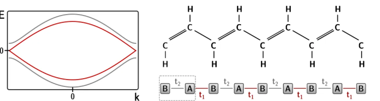
2.4.1 Class DIII:dx2−y2-wave superconductor with Rashba spin-orbit coupling 50 2.4.2 Class AIII/BDI: Su-Schrieffer-Heeger model . . . 53
2.5 Two-dimensional topological insulators and superconductors . . . 55
2.5.1 Dimensional reduction . . . 55
2.5.2 Topological invariants in two dimensions . . . 61
2.6 Summary . . . 66
II Majorana Fermions in disordered quantum wires 67 3 Topological superconductors and Majorana fermions in condensed matter sys- tems 69 3.1 Topological superconductors . . . 69
3.2 Majorana Fermions in condensed matter systems . . . 70
3.2.1 Non-abelian statistics and quantum computing . . . 72
3.2.2 Majorana states in spinless p-wave superconductors . . . . 73
3.2.3 Splitting of edge states . . . 76
3.3 Majorana fermions in real (one-dimensional) life — Quantum wires . . . 77
3.3.1 Clash of parameters — Spin-orbit coupling vs. magnetic field . . . 81
3.4 Experimental observationof Majorana fermions in tunnelling experiments . . 82
4 Quasiclassical theory of disordered multi-channel Majorana quantum wires 85 4.1 Class D spectral peak . . . 86
4.2 Multi-channel quantum wire . . . 88
4.2.1 Hamiltonian of the model . . . 89
4.2.2 Topological band . . . 92
4.2.3 One-dimensional chiral fermions and quasiclassical approximation . . 93
4.2.4 Majorana representation . . . 95
4.2.5 Disorder potential . . . 96
4.3 Quasiclassical approach to multi-channel quantum wires . . . 97
4.3.1 Eilenberger equation and Eilenberger function . . . 97
4.3.2 Density of states . . . 100
4.3.3 Disordered case . . . 102
4.3.4 Single-channel case . . . 103
4.4 Numerical results and discussion . . . 105
4.4.1 Numerical realisation of boundary conditions and disorder potential . 106 4.4.2 Disorder averaged local density of states . . . 106
4.4.3 Sample-to-sample fluctuations . . . 108
4.4.4 Dependence on the magnetic field . . . 108
4.4.5 Mean free path and number of subgap states . . . 111
4.5 Summary . . . 112
4.6 Disorder induced domain walls in quantum wires at criticality . . . 112
Contents
III Appendices 125
A Zero-energy bound states 127
B Chern characters in terms of the Eilenberger functions Q 133
Bibliography 137
Acknowledgement 145
—You know I always wanted to pretend I was an architect.
George Costanza
Introduction
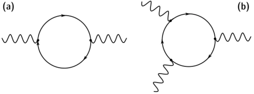
Topological order in condensed matter physics presents a new kind of order for characterising phases of matter. Such phases are described by a global quantity independent of details of the system and are therefore not described within Landaus symmetry-breaking theory. Orig- inating from a ground-breaking work by Thouless et al. [1] in 1982 explaining the integer quantum Hall effect, topological order has become a very important concept of modern condensed matter theory. The study of insulators with topological order, called topological insulators, is a particularly interesting and very active field of research, [2, 3]. An immediate consequence of the topological order in an insulating system is the presence of gapless edge modes. So while the system is an insulator, i.e. there exists an energy gap that separates the valence band from the conduction band, the surface (or edge) of this insulator shows metallic behaviour. The fact that these effects are of topological origin, and as such are insensitive to local perturbations, ensures their stability. Topological insulators are classified by a topolog- ical index which distinguishes insulating phases that are not equivalent, i.e. which cannot be continuously deformed into one another without destroying its defining property, namely the bulk gap. The existence of topological insulators in a given dimension depends on the sym- metries present. They are grouped by symmetries according to the Altland-Zirnbauer (AZ) classification, [4]. It turns out that in each dimension, in five of the ten AZ symmetry classes, topological insulators or superconductors can exist, [3, 5]. For a long time, the presence of time-reversal symmetry in a system was believed to prohibit the possibility to construct a topological insulator. And it was only in 2005 when Kane and Mele, [6, 7] showed that a new type of topological phase can be achieved in the presence of time-reversal symmetry. In two dimensions, this new phase is characterised by helical pairs of edge modes propagating on the boundary of the system. Known as the quantum spin Hall effect, this effect was ex- perimentally observed in 2007, [8]. The concept of topological order was naturally extended to superconductors, described by Bogoliubov-de Gennes Hamiltonians, [9]. This extension is based on the fact that the quasi-particle spectrum is gapped by the superconducting pairing.
Boundary modes in topological superconductors are Majorana particles, i.e. particles that are their own anti-particles, [10]. These quasi-particles are bound to zero-energy and due to their highly non-local nature, are among the most promising candidates for topological quan- tum computing, [11]. Very recent experiments claimed the observation of such Majorana fermions in spin-orbit coupled quantum wires in proximity to an s-wave superconductor and subjected to a magnetic field, [12, 13]. These quantum wires are predicted to host Majorana fermions localised at their ends, [14, 15]. Understanding these wires is critical in identifying Majorana fermions and will be a central topic of this thesis.
In chapter one and three, we review the basic concepts topological insulator and super- conductors as well as the emergence of Majorana fermions in condensed matter systems. In the second chapter we investigate topological insulators in one and two dimensions from a quasiclassical point of view. The quasiclassical technique is a well-established tool in the de- scription of mesoscopic superconductivity, [16–18]. By identifying the relevant information needed to describe the phenomena under investigation, and a subsequent removal of the complementary information, the quasiclassical approach drastically simplifies the involved transport equations. With the characteristic length scales of a superconductor exceeding the Fermi wavelength, the quasiclassical approach confines the Green’s functions to a regime close to the Fermi points by integrating out higher energies. The quasiclassical approach used in this work relies on the fact that close to a topological phase transition, topological insulators and superconductors can be described by a Dirac Hamiltonian which is linear in momentum. We consider disordered one-dimensional quantum wires connected to two topo- logical insulators or superconductors. We present topological invariants for all five symmetry classes in one dimension and determine the number of zero-energy modes localised at the boundary between two topologically distinct phases. It turns out that these invariants solely depend on the quasiclassical Green’s functions at the ends of the quantum wire. In addition, we present the formal solution of the disordered quantum wire, which can be calculated using an efficient numerical method introduced in chapter two. Utilising this approach in chapter four, we show that effects of disorder can lead to signatures which show striking similarities to the ones observed in experiments. We therefore substantiate the scepticism towards the alleged observation of Majorana fermions in the experiments mentioned earlier, [19–21]. Fi- nally, we provide preliminary results on a numerical study regarding the possible formation of topological domain walls due to disorder fluctuations. We consider a one-dimensional quantum wire at criticality and by using the numerical method derived earlier, we investigate the influence of disorder fluctuations on the low-energy properties. In particular, the possible emergence of zero-energy modes, represented by a singularity in the quasi-particle density of states at zero-energy, is explored. These are predicted to form at the boundary between two distinct localised phases.
Part I
Quasiclassical approach to topological insulators and
superconductors
Topological insulators and superconductors 1
Topological insulators and superconductors were recently identified as a very important sub- ject of interest among various branches of condensed matter theory. The point of origin, however, is nowadays considered to be the discovery of the topological origin of the quantised Hall conductance of the quantum Hall effect, already described back in 1982 [1]. In topo- logical insulators and superconductors there exists an intimate correspondence between their insulating bulk and exciting effects at the boundary. Indeed, this correspondence is rooted in the topology of the system which ensures a very robust nature of the boundary effects.
In particular, metallic modes in one dimension that completely evade Anderson localisation exist on the boundary of certain two-dimensional systems.
In this chapter we review the classification of these systems. The classification is based on the identification of equivalent Hamiltonians that can continuously be deformed into one another without destroying the insulating bulk properties, and is a function of dimensionality of the system as well as symmetries present. Famous examples for different types of topo- logical insulators and superconductors, their non-trivial topology as well as their boundary modes are discussed.
1.1 Definition
We start with a rather generic definition of topological insulators or superconductors [3]: A topological insulator or superconductor is a gapped phase of non-interacting fermion sys- tems1 which exhibits boundary modes. These boundary modes are gapless and they are topologically protected, i.e. arbitrary perturbations of the Hamiltonian that do not close the
1Although this restriction can be softened a bit.
bulk gap also do not qualitatively affect these states. However, these perturbations must not render the generic symmetries of the Hamiltonian. A topological insulator or supercon- ductor possesses different phases which are characterised (labelled) by a number, a so-called topological invariant. The nature of this invariant (and therefore their associated phases) depends on the dimensionality and symmetries of the system. It turns out that the invariant either gives an integer or a binary Z2 quantity. As the name implies, these invariants can only change if the phase is changed which in return can only happen if the bulk gap is closed.
The latter can be understood by a very intuitive argument: Consider two insulators at- tached to each other, we ignore the trivial case in which both are trivial insulators or topolog- ical insulators with the same value of the invariant. The remaining two cases will always be separated by a boundary. This boundary however will host gapless boundary modes, which implies a gap closure. Hence one cannot interpolate between both systems without closing the band gap at the boundary. By the same token, systems with the same invariant are topologically equivalent and can be deformed smoothly into one another without closing the gap.
Simply put, a classification of topological insulators and superconductors has been es- tablished by determining the classes of topological insulators and superconductors that can continuously be transformed into one another without closing the gap, and are thus described by the same quantity/invariant.
A frequently used example for such a topological invariant in mathematics is the Euler characteristic. In the simplest case of a closed orientable surface this invariant is a linear function of the number of holes, the genus, within this surface. The Gauss-Bonnet theorem then ensures that smooth deformations (not changing the number of holes) of the surface will leave this characteristic unchanged [22]. An analogy to this theorem will be given later.
1.2 Symmetry classes - The ten fold way
For non-interacting disordered fermion systems there exist a classification due to Altland and Zirnbauer [4, 23]. The classification is based on the presence or absence of three generic symmetries: time-reversal symmetry (T), charge-conjugation (or particle-hole) symmetry (C) and a third, chiral (or sublattice) symmetry (S). The Hamiltonians under consideration are not translationally invariant and the symmetries are represented by anti-unitary operators which commute with the Hamiltonian of the system.2
Let H be the N-dimensional first quantised Hamiltonian of our quantum system, repre- sented by a matrix of dimension N ×N. For both, time-reversal and charge-conjugation symmetry the anti-unitary operators can be represented as a product of a unitary operator (UT or UC, respectively) and an anti-unitary operator. The latter is frequently chosen as
2Note that translational invariant symmetries, i.e. unitary symmetries that commute with the Hamiltonian have to be excluded. If such a unitary symmetry is present, the Hamiltonian is always block-diagonalisable (reducible). For the classification one thus only considers irreducible representations of the Hamiltonians.
1.2 Symmetry classes - The ten fold way
complex conjugation operator K, i.e.T =K·UT and equivalently forC.
The system is time-reversal invariant if H commutes with the time reversal symmetry operator, i.e.
UT†HTUT =H. (1.1)
By the same token, a system is charge-conjugation invariant if
UC†HTUC =−H. (1.2)
In addition to the two symmetry operations above, the product of both symmetry op- erations S = T ·C gives rise to a third symmetry. A system possesses chiral symmetry if
US†HUS =−H, (1.3)
i.e. if H anti-commutes with the unitary matrix US = UT ·UC∗. Note that although the product of both symmetries is a unitary operation, the fact that H and US anti-commute spoils the triviality of this symmetry (its reducibility). However, for two distinct time-reversal (charge-conjugation) operatorsTi=1,2 (Ci=1,2), the subsequent application of two symmetry operations will be a unitary operation that commutes withH, and hence will be discarded.
The products U∗U, for U = UC or UT, are at this point not further specified, however they both obviously commute withH. Since we excluded unitary symmetries that commute with H, we are dealing with an irreducible representation of the latter, hence Schur’s lemma ensures that the product U∗U of two unitary matrices is the identity up to a sign,
U∗U =±1. (1.4)
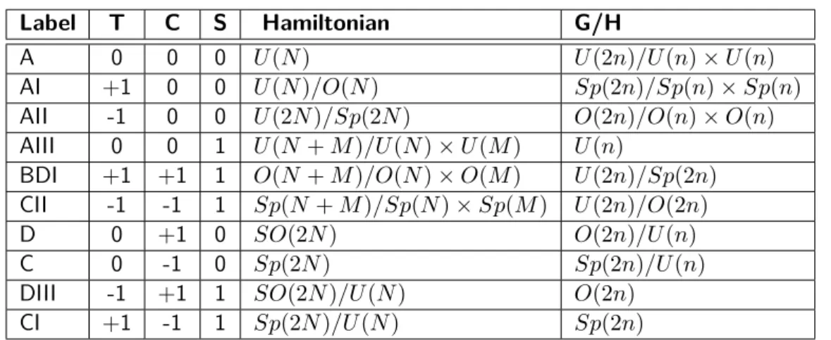
By simply counting the possible combinations we conclude that there are ten different classes (all possible combinations of T and C will lead to nine classes, however in the absence of both, S can still be present filling the missing spot). The ten symmetry classes are comprised in table 1.1, where the 0 entries indicate the absence of a symmetry and ±1 entries refer to the sign in eq. (1.4).
Having identified the ten possible symmetry configurations the question regarding the exhaustion of this scheme was answered by the authors of refs. [4, 23]. We will address this question together with some physical remarks by further inspecting table 1.1. The first column labels the symmetry classes in a way that will be explained later. One immediately recognises the original Wigner and Dyson classes A, AI and AII for random matrices. These classes are naturally extended by inducing the chiral symmetry and are therefore called chiral classes, AIII, BDI and CII. The remaining four symmetry classes (D, C, DIII, and CI) are found to be realised in disordered superconducting systems described by Bogoliubov-de Gennes Hamiltonians [4].
Label T C S Hamiltonian G/H
A 0 0 0 U(N) U(2n)/U(n)×U(n)
AI +1 0 0 U(N)/O(N) Sp(2n)/Sp(n)×Sp(n)
AII -1 0 0 U(2N)/Sp(2N) O(2n)/O(n)×O(n) AIII 0 0 1 U(N+M)/U(N)×U(M) U(n)
BDI +1 +1 1 O(N+M)/O(N)×O(M) U(2n)/Sp(2n) CII -1 -1 1 Sp(N +M)/Sp(N)×Sp(M) U(2n)/O(2n)
D 0 +1 0 SO(2N) O(2n)/U(n)
C 0 -1 0 Sp(2N) Sp(2n)/U(n)
DIII -1 +1 1 SO(2N)/U(N) O(2n)
CI +1 -1 1 Sp(2N)/U(N) Sp(2n)
Table 1.1: Altland-Zirnbauer classification of random matrix ensembles. Symmetry classes are labelled due to Cartan (first column). The presence or absence of time-reversal (T), charge-conjugation (C) and sublattice symmetry (S) are indicated by±1and 0, respectively. The fourth column lists the symmetric space of exp(iH), while the fifth column shows the target spaces of the non-linear-sigma-model (see text for explanation). Table taken from [4].
The fourth and fifth column in table 1.1 is related to the completeness of this list of classes. We consider the first quantised Hamiltonian H to be represented as an N ×N matrix and construct the objectX=iH, as well asexp{X}. Formally the former object is an element of an algebra, while the latter is an element of a corresponding coset space [4].
Physically, the latter object can be interpreted as the quantum mechanical time-evolution operator exp{iHt}. For each class, the symmetries impose restrictions on the structure of H (and thus the full algebra is restricted to a sub-algebra thereof) and consequently on the time-evolution operator and its coset space. These coset spaces are summarised in the fourth column of the table.
A few simple examples should clarify this point. Consider class A, i.e. since no symmetries are present, H is simply a hermitian matrix. Consequently X is skew-hermitian, i.e. X† =
−X. SinceXandX†trivially commute with each other, it follows thatexp{X}exp{X}†= id. Hence exp{x} is an element of the Lie group U(N). It is obvious that upon further restricting our system, the Hamiltonians have to be restricted to subsets. In fact for class AI, the Hamiltonian can be represented as a real symmetric matrix, i.e.H=HT. The coset space turns out to be given by the quotient U(N)/O(N). To this end, one realises that each hermitian matrix can be decomposed into a real symmetric and skew-symmetric part, H = Hs+iHa. If we construct the likewise skew-symmetric Xa = iHa, it follows that exp{X}exp{X}T = id and hence exp{X} ∈ O(N). The coset space of real symmetric matrices is thus the coset space U(N)/O(N), as indicated in table 1.1. The remaining entries of the classification table are constructed accordingly.
1.3 Classification table of topological Insulators
Label /d 0 1 2 3 4 5 6 7 8
A Z 0 Z 0 Z 0 Z 0 Z
AIII 0 Z 0 Z 0 Z 0 Z 0
AI Z 0 0 0 2Z 0 Z2 Z2 Z
BDI Z2 Z 0 0 0 2Z 0 Z2 Z2
D Z2 Z2 Z 0 0 0 2Z 0 Z2
DIII 0 Z2 Z2 Z 0 0 0 2Z 0
AII 2Z 0 Z2 Z2 Z 0 0 0 2Z
CII 0 2Z 0 Z2 Z2 Z 0 0 0
C 0 0 2Z 0 Z2 Z2 Z 0 0
CI 0 0 0 2Z 0 Z2 Z2 Z 0
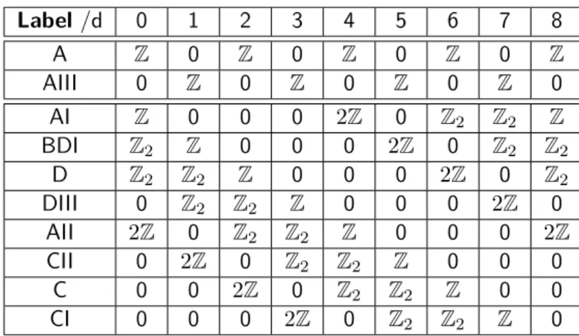
Table 1.2: Classification of topological insulators and superconductors. Symmetry classes are again labelled by the Cartan labels and rearranged. Depending on the dimension d, a trivial insulator or superconductor exists (Z or Z2) or not (0). The non- zero entries indicate that the topological phases present are characterised by aZ2
invariant or an integer (Z). Table can be found in [3].
The completeness of this table was established by realising that the entries in the fourth column agree with a set of mathematical objects, called symmetric spaces. Details are not of interest at this point and beyond the scope of this text, however it was shown by Cartan in 1926 [24] that this set includes only ten symmetric spaces. This proves that the classification is exhausted and explains (within this framework) the notation used in the first column of table 1.1. The fifth column is related to the physics of Anderson localisation at long wavelength, which can described by a non-linear-sigma-model. The target space of these systems, again turn out to be given by the ten symmetric spaces.
1.3 Classification table of topological Insulators
Table 1.2 shows the classification table of topological insulators and superconductors. The classification is based on the ten symmetry classes of random Hamiltonians presented in the previous section. The entries Z,Z2 and 0 indicate whether in the corresponding symmetry class, for a given dimension d, the existing phases are characterized by an integer, a binary quantity or are absent at all, respectively. How the corresponding invariants are constructed in details depends on the specific model chosen. The symmetry classes in table 1.2 are re-organised in a way to reveal its periodicity. The classification shows a regular pattern composed of a sequence of (2Z,0,Z2,Z2,Z), that is periodic (modulo 8) in the dimen- sionality. This so-called Bott periodicity [25] is closely related to the reappearance of the symmetric spaces and its mathematical origin goes beyond the scope of this work.
Before elaborating on the specific realisations for the different entries of this table, we
will briefly discuss the structure behind it and comment on the genesis of it. Due to the formal nature of this discussion, readers desperately longing for a concrete physical model may unhesitatingly skip the remainder of this section.
Classification schemes
The classification table 1.2 has been derived by various means [3, 5, 26]. All classifica- tion schemes are related to the symmetric spaces discussed earlier and have an underlying mathematical framework:
Absence of Anderson localisation at the boundary - NLσM classification
In the definition of a topological insulator or superconductor given at the beginning of this chapter, a basic ingredient was the existence of gapless edge modes at the boundary of the system. Being of topological origin, these states are protected against disorder and other backscattering effects. This obtrudes the interpretation of the (d−1)-dimensional boundary of ad-dimensional topological insulator or superconductor, as a metal that evades Anderson localisation. In ref. [26] it was studied what topological terms can be added to the non-linear-sigma-model (NLσM), describing Anderson localisation on the boundary of a topological insulator, which evades this phenomenon. It turns out, that only two types of terms can be added: a Wess-Zumino-Witten or aZ2-term. This result is determined by the homotopy groups of the target space (again represented by the ten symmetric spaces and presented in the fifth column in table 1.1). The homotopy groups are eitherπd=Zor πd−1 =Z2, respectively. A classification of topological insulators and superconductors thus breaks down to the well known table of homotopy groups for the symmetric spaces.
Projectors - Grassmanian classification
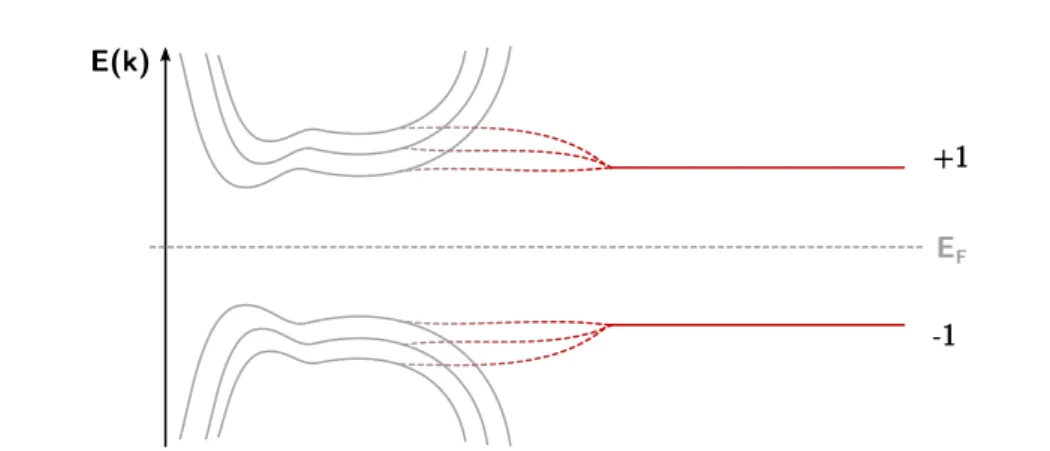
Given a topological insulator the ground state is given by the filled bands below the Fermi energy in the Brillouin zone. With the eigenstates of the Hamiltonian above and below the Fermi energy well separated by the bulk gap, it is common to flatten the bands on both sides of the gap [3, 27]. As long as the bulk gap is not closed, the Hamiltonian can always be continuously deformed into one with unique eigenvalues +1 and −1, above and below the gap respectively. This deformed Hamiltonian is usually called flattened or simplified Hamiltonian. Note that the eigenstates are not changed and since it can be shown that topological properties do not depend on the energies of the occupied bands but only on the eigenstates, the flattened Hamiltonian allows for simplified calculations. The procedure of flattening is illustrated in fig. 1.1.
The flattened Hamiltonian in momentum space is defined as Q(k) = 1−2P(k),
1.3 Classification table of topological Insulators E(k)
EF +1
-1
Figure 1.1: Flattening of a generic band insulator. The bands Ea(k) (grey curves) are con- tinuously deformed to E±=±1 (red curves) without closing the band gap.
where P(k) = Pa|u−a(k)ihu−a(k)| is the spectral projector onto the filled bands, and {|u−a(k)i} denotes the set of filled Bloch wave functions with (occupied) band index a.
We denote bynthe number of bands below the gap, i.e. with energyEa(k) =−1and bym the number of bands above the gap with energiesEa(k) = +1. With no symmetries present, the flattened Hamiltonian Q(k) is a map from the Brillouin zone to the set of eigenvectors, i.e. U(n+m). However, there exists an intrinsic gauge symmetry due to the possibility of relabelling the nfilled andm empty states. Thus Q(k) is a map from the Brillouin zone to U(n+m)/(U(n)×U(m)) =:Gm,m+n(C), the complex Grassmannian. For a classification of topological insulators and superconductors, two ground states of different classes should not be able to be deformed into one another without closing the gap. Thus, it is again the homotopy group of the target spaces of the flattened Hamiltonian Q(k) that is used to identify the phases.
Considering class A, i.e. no symmetries present, we have already seen that the target space ofQ(k)isGm,m+n(C). To find out whether or not the symmetry class in a given dimension is topologically trivial, we rely on well known results on homotopy groups. In the present case it turns out that π2(Gn,n+m(C)) = Z whileπ3(Gn,n+m(C)) = {id}, i.e. while in two dimensions there exist Z topological phases in one dimension higher none exists.
In the presence of symmetries, the space of projectors will be further restricted. In case of a present chiral symmetry (such as in class AIII) the projector can always be brought into block off-diagonal form
Q(k) = q q†
! .
SinceQ2=1, it follows thatq has to be unitary,q∈U(m). The homotopy groups ofU(m) areπd∈2N(U(m)) ={id}andπd∈2N+1(U(m)) =Z, i.e. trivial in even and non-trivial in odd dimensions.
Subsequently, a complete classification table based on the homotopy groups of the space of projectors can be constructed, which of course is equivalent to tab. 1.2. The reappearance of the ten symmetric spaces is revealed by considering the projectors in a zero-dimensional momentum space, or at invariant points of the Brillouin zone related by time-reversal or charge-conjugation symmetry. In this case, the spaces of projectors again turn out to be exactly the ten symmetric spaces discussed earlier. On passing we note that an equiva- lent classification was achieved using Clifford algebras and K-theory, revealing the spaces of projectors as the classifying spaces used in K-Theory [5].
The above discussion shows that the nature of the insulator is fully encoded in the pro- jectors Q(k). As a map from the Brillouin zone to some Grassmannian it assigns to each momentum vectorka transformation to the eigenstates. Understanding this transformation implies understanding the topology of the insulator. If this transformation can continuously be transformed to a trivial transformation3, the insulator is trivial. On the other hand, if the transformation is not homotopic to the identity, the insulator is topologically non-trivial.
1.4 Chern number and the integer quantum Hall effect
Let us continue by introducing a well known model and thereby shine some light on the formal discussion of the previous subsections. We have learned that there exists a classification table which tells us the symmetry class (and dimension) necessary to find topological insulator or superconductor. We were also told by which type of quantity the topological phases are labelled. How this labelling, i.e. the construction of the topological invariant, is done in detail will be explained next using the example of theinteger quantum Hall effect (IQHE).
Indeed the IQHE is now considered to be one of the first theoretical emergences of a topological insulator. In a seminal work [1], Thouless et al., showed that the transverse Hall conductivity σxy is quantised. Moreover, the authors realised that the origin of this quantisation was routed in the topology of the bulk of the system. For the IQHE, electrons are confined to a two dimensional plane and subject to a strong magnetic field, thus neither time-reversal nor particle-hole symmetry are present. According to table 1.1 the system is a member of class A, and table 1.2 reveals that in two dimensions the phases are indeed quantised (Z). It turns out that the quantisation of the Hall conductance is described by the (first) Chern number C1. The Chern number is a topological invariant, hence two Hamiltonians that cannot be continuously deformed into one another without closing the gap, cannot give the same value of the invariant. More precisely, the Hall conductivity is given by
σxy =C1e2/h.
Before we construct the first Chern number explicitly, we should pause and embrace this
3Notice that we used{id}as the set that contains only the identity element and hence the transformation was trivial.
1.4 Chern number and the integer quantum Hall effect
seemingly innocent result. The Hall conductance can straightforwardly be calculated by means of linear response theory and is a real, measurable quantity [28]. The result above is purely geometrical and hence this quantisation is robust. Thereby, the non-trivial ge- ometry of the topological insulator ensures the robustness of an experimentally measurable quantity, a canonical scheme of topological insulators usually referred to as bulk-boundary correspondence.
We now aim to construct the integer invariant and offer two common interpretations of the result. The quantisation of circulating electrons lead to quantised Landau levels En = ~ωc(n+ 12), with cyclotron frequency ωc. Although it is not possible for the states to be labelled with their momentum, a band structure can be constructed by choosing a proper unit cell. This allows for the application of Bloch’s theorem and the labelling of the states with a two-dimensional crystal momentum. The energy levels are then given by the Landau levels, En(k) =En. A bulk energy gap is present if, say N of these Landau level are filled while the remaining ones are empty, the band structure is thus equivalent to one of an insulator.
Given the band structure, a flattened Hamiltonian Q(k) is easily defined. The effective Hilbert space is Hk∼=C2N ifN denotes the total number of Bloch wavefunctions, and the Brillouin zone is a two-dimensional torusT2. However, since we are interested in the flattened Hamiltonian, we can choose N = 2for simplicity with one occupied and one empty band.
We have already learned that Q(k) assigns to each (quasi-)momentum k an eigenvector
|u−(k)iand that these states posses aU(1)gauge-freedom, as they are only defined up to a quantum mechanical phase. A state is thus represented by an equivalence class[|u−(k)i] :=
{g|u−(k)i : g ∈ U(1)}. The collection of all Hk constitutes a mathematical object called vector bundle4 over the base spaceT2, denoted by P(T2, U(1)). The group gacting on the states is called structure group, and acts by left multiplication. The bundle comes with a projection π (see fig. 1.2) whose inverse image maps from the torus to the fibres [|u−(k)i].
Notice that the structure group and the fibres are both (isomorphic to)U(1), and hence the vector bundle is called a principle bundle.
Pictorially speaking, a bundle is called trivial if it can globally be written as a direct product of its base space (in our case T2) and the fibre. The word globally is very important at this point. A non-trivial bundle although locally a direct product space, cannot be written as one globally.
On this bundle the Berry connection [29]5,
a(k) =aµ(k)dkµ:=ihu−(k)|du−(k)i=−ihdu−(k)|u−(k)i,
can be constructed, where the exterior derivative is defined as d = (∂kµ)dkµ. Note that
4More precisely a principal bundle [22].
5Sloppily speaking, a connection is a unique decomposition of the bundles tangent space into a horizontal and vertical subspace, that allows for directional derivatives of vector fields. Physically, the corresponding form can be thought of as a vector potential.
k g
Figure 1.2: Principal bundle over the Brillouin torusT2. The structure group g acts by left multiplication on elements|u−(k)iof the fibre'π−1(k). The projectionπmaps from the fibre onto the base space given by the torus T2.
the Chern number does not depend on the specifically chosen connection. Given the Berry connectiona, the Berry curvature is defined as6
F = da=Fµνdkµ∧dkν :=ihdu−(k)| ∧ |du−(k)i. (1.5) At this point we recall the previously mentioned Gauss-Bonnet theorem which connected the integral of the (Gaussian) curvature over a closed surface to an integer (in units ofπ), which in return was related to the holes in the manifold. The natural generalisation of this theorem identifies the first Chern number
C1 = 1 2π
Z
BZ=T2
F, (1.6)
with an integer. As two manifolds of different genus cannot be continuously deformed into one another without punching or closing a hole, a difference in the Chern number indicates that two systems are topologically distinct and only through closing the band gap can they be transformed into one another.
Two geometrical interpretations of the above statement can be illustrated by conveniently choosing the simplest model of a two-band insulator. The Hamiltonian we consider is given by
H(k) =
3
X
i=1
hi(k)σi, (1.7)
where thehi(k) are real, periodic functions andσi=1,2,3 are the Pauli matrices representing the (pseudo)-spin degree of freedom. In the above model we ignore trivial contributions
6Ifais interpreted as a vector potential,F would analogously be interpreted as a magnetic field.
1.4 Chern number and the integer quantum Hall effect
proportional to σ0 = 1 since they merely lead to a shift in energy. We again denote the eigenstates of the upper and lower band by |u±(k)i and the energies of both bands are given by ± = ±qPih2i ≡ ±|h|. The band gap does not close as long as |h| 6= 0.
As usual, we concentrate on the lower filled band |u−(k)i. ˆh = h/|h| then defines a map from the Brillouin torus to the sphere S2 and the filled eigenstates take the polar- representation7 |ui= (−sin Θ/2,exp[iφ] cos Θ/2)T. LetH(k)be given such that atk= 0, ˆh is pointing at the north pole8 (Θ = 0) the eigenvector |ui is not well-defined because of the arbitrary phase exp[iφ]. However, if the vector stays in the southern hemisphereUS of S2, the eigenvector |uSi = |ui is well-defined. A well-defined eigenvector on the northern hemisphere UN is easily constructed, |uNi = exp[−iφ]|uSi. A natural question to ask is what happens at the equator, i.e. the non-vanishing intersection which surges the northern hemisphere, ∂UN =UNTUS 'S1? At the transition we can define a transition function g : ∂UN → U(1) (notice the reappearance of the structure group U(1)) that defines the phase change by g = exp[iφ]. The topology of the bundle can thus be described by the behaviour of the transition functiong. Ifˆhdoes not cover the whole sphere, the eigenvector of the corresponding hemisphere can be globally defined and the transition function is trivial g 'idS2. If, however,ˆh ends up covering the whole sphere, the transition function cannot be transformed to the identity and the topology of the bundle is non-trivial. In the latter case it is not possible to construct a global eigenvector on the whole sphere [30]. Indeed it is straightforward to see that the Chern number (1.6) is given by
C1= 1 2πi
Z
∂ˆh−1(UN)
d log(ˆh?g), (1.8)
i.e. the winding number of the transition function g. Since the construction of a global eigenvector is only possible ifg is homotopic to the identity, the Chern number is vanishing C1 = 0. In contrast, a non-vanishing Chern numberC1 6= 0indicates a non-trivial transition functiongand an obstruction to define a global eigenvector. For the explicit two-band model, the first Chern number can straightforwardly computed by explicitly evaluating eqs. (1.5) and (1.6), and is given by9
C1 = 1 4π
Z
T2
h|h|−3·∂kxh×∂kyhdkx∧dky. (1.9) Consider a closed loop in the Brillouin zone, under the map ˆh : T2 → S2 this loop will describe a closed surface S in the hx, hy plane and since the system is gapped, a winding
7We drop the superscript since we only consider the lower filled band.
8Notice that multiplication by the inverseexp[−iφ]would merely shift this singularity to the south pole at Θ =π.
9We went with a very sloppy yet common notationijkhidhj∧dhk= 2h·(∂xh×∂yh)dkx∧dky, i.e. we introduced an artificial cross-product in two dimensions. The latter representation is commonly used in literature ignorant of exterior calculus [31].
number around the origin can be associated to it. The Chern number is exactly this winding number defined in eqs. (1.8) and (1.9). If we project the sphere down to R3 \ {0}, this winding number counts the number of times the closed surfaceS wraps around the origin.
In case of a trivial system, S does not contain the origin and the winding is thus trivial C1 = 0, which corresponds to the previously discussed scenario in which ˆh does not explore the whole sphere but stays in one hemisphere. Whereas in the case of a non-vanishing winding numberC1 6= 0, the map explorers the whole sphere (with a non-trivial transition).
Figure 1.3 illustrates the map hˆ and corresponding surface on S2. In a more physical interpretation eq. (1.6) defines a flux through the Brillouin zone. The source of this flux is revealed by eq. (1.9), sinceh|h|−3 defines the field of a point-like magnetic monopole at the originh= 0. Placed within the torus the flux is non-vanishing, while a monopole outside of the torus contributes to no total flux.
S
Figure 1.3: Map from the Brillouin torus to the Bloch sphere S2. A closed loop on T2 is mapped to a surfaceS onS2.
1.5 Dirac Hamiltonians
We return to the generic two-level Hamiltonian H(k) = ˆh·σ =
3
X
i=1
hˆi(k)σi, (1.10)
where we defined the three-dimensional vectorsˆh= (ˆh1,ˆh2,ˆh3)andσ= (σ1, σ2, σ3)T. The vectorhˆ again defines a map from the Brillouin zone (the torusT2) to the sphere S2, as it was discussed in the previous section.
Possible time-reversal symmetry restricts the choice of ˆhi depending on the nature of σ.
If the Pauli matrices constitute a basis for a system with pseudo-spin (T2 = +1), it follows trivially thathˆ1 andˆh3 have to be even functions ink, whereas ˆh2 has to be odd. According to eq. (1.9), the Chern number has to vanish. For a system with real spin degrees of freedom
1.6 Haldane model
(T2 = −1), in order to preserve time-reversal symmetry allhˆi have to odd functions in k.
Consequently the system has to be gapless.
In the vicinity of a point of gap closure (such as at time-reversal invariant momenta), the Hamiltonian (1.10) can be linearised leading to a two-dimensional Dirac Hamiltonian.
These points are frequently referred to as Dirac points. The generic form of a massive Dirac Hamiltonian is achieved10 by replacing ˆhi=1,2 →k1,2 andˆh3 →m in eq. (1.10),
H(k) =
2
X
i=1
kiσi+mσ3. (1.11)
The dispersion E(k) =±√
k2+m2 exhibits a gap of2|m|. For the massive Dirac Hamilto- nian the Chern number of the filled band is given by
C1 = 1 2π
Z
T2
m 2
m2+k2−3/2dk= sgnm/2.
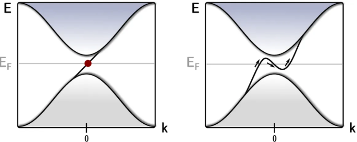
Surprisingly the Chern number and thus the Hall conductance turns out to be a half integer, which contradicts our statements earlier. Indeed we cheated in stating that the Chern number always has to be an integer and indeed the linear dispersion of the Dirac Hamiltonian serves as a perfect counter example. The reason behind this is rooted in the fact that the dispersion stays linear in the limit|k| → ∞and the integration manifold is non-compact and effectively halved, leading to the half-integer result [3]. The integer result is always true on a lattice, for a continuum model, however, a regularisation of the mass, which annihilates the linear dispersion in the large k limit, is necessary. Although the full Chern number can only be obtained by integrating over the full Brillouin zone, an integer change in the invariant is still present within the Dirac description. A sign change in the mass of the Dirac Hamiltonian thus indicates a transition, which necessarily involves a closing of the gap. Figure 1.4 illustrates the dispersion around the Dirac points and the change of the Chern number as a function of mass. Dirac Hamiltonians with linear dispersion will cross our paths again in the second part of this work, where the linearisation is used to formulate a quasiclassical description of topological insulators and superconductors.
1.6 Haldane model
Haldane [32] demonstrated that a non-trivial two-band insulator with a quantised Hall con- ductance can be realised in a honeycomb lattice with two inequivalent sub-lattices in the absence of an external magnetic field. In order to break the time-reversal symmetry the model requires a local magnetic flux that only affects second neighbour hopping amplitudes,
10In order to avoid confusion, we linearise the two level Hamiltonian around a momentum, sayq, close to the Dirac point. By setting both~and the Fermi velocityvF to unity and redefiningq→kwe end up with eq. (1.11).
C=1
Figure 1.4: Schematic dispersion for topological insulators with different Chern numbers (in- dicated by red curve). At the Dirac point, the gap closes in a linear manner and the Chern number signalises an integer jump∆C.
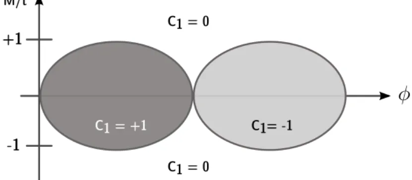
with a vanishing net flux per unit cell. The system possesses two Dirac points around which the linearised Hamiltonian is given by eq. (1.11), and the mass terms at this two points are m =M ±tsinφ, where ±M are the on-site energies of the sub-lattices, t is the hopping amplitude andφthe Aharnov-Bohm phase (induced by the local flux [32]). Modulating the two parameters M and φ the phase diagram of the Haldane model (fig. 1.5) can be con- structed. One recognises two phases (|M|< tsinφ) corresponding to a positive and negative Chern number (coloured areas) and a third trivial phase (|M|> tsinφ) corresponding to a vanishing Chern number. The gap vanishes at the Dirac points but a finite gap evolves as a function of both parameters, separating all three phases. The transition lines (|M|=tsinφ) separating these phases indicate the parameter values for which the system is no longer an insulator.
M/t
C1 = +1 C1= -1
C1 = 0 C1 = 0 +1
-1
Figure 1.5: Phase diagram for the Haldane model. The system is in the trivial phase (C1 = 0) for |M/t|>sinφand in the non-trival (C1 =±1) for |M/t|<sinφ. The lines
|M/t|= sinφ indicate phase transitions at which the bulk gap closes.
1.7 Edge states
1.7 Edge states
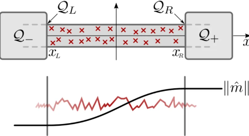
By definition, a topological insulator hosts metallic surface states at its boundary. On several occasions we have seen, that a gap closing has to occur on the boundary between two insulators with different values of the topological invariants. For Dirac Hamiltonians we now illustrate that one can indeed prove the existence of such states by simple arguments. To this end, we consider an interface between two topological insulators described by a massive Dirac Hamiltonian (such as the Haldane model). On the left-hand side the insulator is supposed to be trivial (C1 = 0) while on the right-hand side it is non-trivial (C1 = 1). As we have seen, such a change in the Chern number can only be achieved by a sign change of the mass across the interface, as illustrated in fig. 1.6. In order to describe the edge state sitting at the interface where the mass vanishes, one solves the corresponding Schrödinger equation in real space for the massive Dirac Hamiltonian. A detailed derivation is done in [2] leading to the normalised solution
Ψ(x, y)∝exp[ikxx] exp[−
y
Z
0
m(y0)dy0](1,1)T, (1.12) where the mass changes sign along the y-axis and vanishes aty = 0. The eigenenergy (in units of ~ =vF = 1 and for EF = 0) is given by E(kx) = kx. Thus eq. (1.12) describes a chiral (moving only in one direction) state, that transversely crosses the interface (in x- direction) with a positive Fermi velocity. In fig. 1.7 this single state connecting the valence and conduction band is illustrated.
C
1=0 C
2=+1 +1
-1
y=0
Figure 1.6: Schematic illustration of an interface between a trivial insulator (left) and a non- trivial one (right). The sign of the mass term in the Dirac Hamiltonian changes (black lines) from −1 to +1 at the interface (y = 0). The red curve represents the wave function of the localised zero energy mode at the interface. Details are explained in the text.
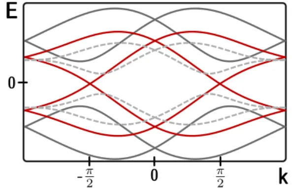
We have yet encountered another example of the bulk boundary correspondence. Of course, the procedure above is not tied to Dirac Hamiltonians and the idealised band structure in fig. 1.7 might become more complicated. The Fermi energy could in general intersect with the connecting band several times. In case of an edge state, it will always cross it an odd number of times and for each intersection the direction of the Fermi velocity needs to be taken into account. As a consequence, the weighted sum of all intersections will always equal the change in Chern numbers across the interface at which the transition happens.
0
k
E E
F0
k
E E
FFigure 1.7: Chiral edge state crossing the Fermi energy. Left: The edge state crosses the Fermi energy once with positive group velocity. Right: The band of the chiral edge state crosses the Fermi energy three times. Twice with positive and once with negative group velocity. The direction of the velocity is indicated by arrows.
1.8 Z2-topological insulators
The above arguments lead to a vanishing Chern number in the presence of time-reversal symmetry. It was shown by Kane and Mele [6, 7], that for a system with half integer spin, spin-orbit interactions open a possibility for a topologically non-trivial system with unbroken time-reversal symmetry. Although the Chern number is always trivial, the phases can be classified by a topological Z2 invariant. The authors considered graphene described by a Haldane model but replaced the local magnetic flux by spin-orbit interactions. The physical phase distinguished by theZ2-invariant is called thequantum spin Hall effect (QSHE). Note that these results were independently derived by Zhanget al.[33, 34]. Where the QSHE was predicted in HgTe quantum wells, which was experimental confirmed shortly thereafter [8].
The presence of time-reversal symmetry relates a Bloch states at k to the one at −k and thus the time-reversal operator defines an anti-unitary map from the fibre atk to the fibre at−k. And indeed, the valence bundle turns out to be always trivial considering the Chern number and the constraints imposed on the eigenstates reveal the non-triviality of the
1.8 Z2-topological insulators
system [30].
Due to Kramer’s theorem all eigenstates of the Hamiltonian are at least two-fold de- generate. Spin-orbit coupling splits this degeneracy except for isolated points called time- reversal-invariant moments (TRIM). These points are located at the boundary of the effective Brillouin zones11. The binary nature of the classification can be understood from a very sim- ple picture: Since the eigenstates are degenerate at the TRIM, depending on the system, a band connecting the valence and conductance band may intersect with the Fermi energy even or odd times. The former case is trivial since the system can be continuously deformed (imagine lifting the band above the Fermi energy) and the intersection can be removed, leaving the dispersion with no band connecting the valence and conductance band. In case of an odd number of intersections this is not possible and the system is non-trivial, exhibiting an edge mode. Recall that in the case of a Chern insulator the weighted number of times the connecting band intersects with the Fermi energy, defined the change in the Chern number.
In case of the QSHE, the number of Kramers pairs of the edge mode that intersects with the Fermi energy defines the change in a Z2 invariant. Before we consider the nature of these edge modes, we elaborate a bit more on the construction of the invariant. Similar to the discussion for Chern insulators, the obstruction to construct a basis on the whole Brillouin zone, where the eigenstates are related by the time-reversal operator, proves to be impossible in the non-trivial case. Details can be found in ref. [30]. There are several ways to define a Z2 invariant [7, 35], one that will be of interest at a later stage was introduced by Fu and Kane [35]. The sewing matrix is defined as
w(k) =hum(k)|T un(−k)i,
where|u(k)iagain denote the occupied Bloch functions andT the anti-unitary time-reversal operator with T2 = −1. w measures the overlap or orthogonality of the Bloch states with their time-reversal partners. It is unitary and furthermore at the TRIM, w is skew- symmetric wT = −w. A skew-symmetric matrix allows for the definition of a Pfaffian, Pf(w) = (detw)2. Thus for each TRIM ka we can define the binary quantity
δa= Pf(w(ka)) det(w(ka))−12 =±1,
and if the Bloch states are chosen continuously, theZ2 invariant is defined as (−1)ν =Y
a
δa, (1.13)
where the product runs over all TRIM (of which there are four in two dimensions).
The edge states of the QSHE can be derived in the same fashion as for the IQHE. The simplest model necessarily involves four levels (two levels with different spin). The Hamilto-
11Since time-reversal symmetry is present it is sufficient to only consider half of the Brillouin zone.
nian (1.7) thus has to be represented in a four-dimensional basis and is given by H(k) =
5
X
i=1
hi(k)Γi+X
i>j
hij(k)Γij,
where the gamma matricesΓi=1,...,5 obey the Clifford algebra12 [Γi,Γj]+ = 2δij and Γij =
−2i[Γi,Γj]−. Symmetry constraints opposed to the system restrict the gamma matrices further.
Considering the model introduced by Kane and Mele, a linearisation around one of the TRIM, as it was done in the discussion on Dirac Hamiltonians for Chern insulators, leads to the minimal representation
H(k)'k1Γ5−k2Γ2+mΓ1,
where we again assume that the sign of the massmchanges along a coordinateyand vanishes at the interface between two different insulators aty= 0. The specific representation of the gamma matrices are of no importance at this point and will be discussed later; it is sufficient to understand that they live in the tensor space of spins and the degrees of freedom of the two-level system13. However, it is easy to see that the Hamiltonian can be block diagonalised with each block referring two one of the two spin species,H = diag(H↑, H↓) and thus the Schrödinger equations decouples within the spins. These Schrödinger equations are then straightforwardly solved in real space [30], yielding
Ψ↑/↓(x, y)∝exp[∓ikxx] exp[−
y
Z
0
m(y0)dy0]ˆe↑/↓,
whereeˆ↑ = (0,1,0,0)T andeˆ↓ = (σ1⊗1) ˆe↑. Thus the boundary hosts helical edge states, one state with spin-up moves to the right and the spin-reversed partner moves to the left with the same velocity. These helical edge states are illustrated in fig. 1.8 and the parities of these helical edge states are represented by theZ2 invariant eq. (1.13).
1.9 Stability of edge states
The robustness of metallic edge states, present due to the bulk boundary correspondence, is protected due to their topological origin. Chiral and helical edge states have been identified at the boundary of a Chern and Z2 topological insulator, respectively. Chiral edge modes only travel in one direction and simply put, there is just no possibility for backscattering as long as the sample width is larger than the decay length of the edge mode [36]. For
12Throughout this work we denote (anti-)commutators by[A, B]ξ=A◦B+ (ξ)B◦A.
13Therefore they are in general a tensor product of two Pauli matrices.
1.10 Topological superconductors
0
k
E E
FFigure 1.8: Helical edge states of the QSHE. A pair of electrons moving in opposite directions with opposite spin cross the Fermi energy.
the helical edge states in the QSHE the robustness is due to destructive interference of the backscattering paths. Imagine an electron with spin σ travelling along the edge of the QSH insulator. We assume that there is only one pair of edge states. If the electron is reflected by disorder compatible with the symmetry class (i.e. non-magnetic disorder), it has to flip its spin (since it is helical). The two possible paths (illustrated in fig. 1.9) the electron can take during that scatter process will rotate the spin by an angle of ±π, depending on which direction it takes, resulting in a total difference of 2π between both paths. Thus for half-integer spin, both paths will interfere destructively14. Therefore the presence of time- reversal symmetry protects the edge states by annihilating the possibility of backscattering.
On a final note we see that the parity of helical states at one edge indeed relates to the Z2 invariant eq. (1.13), as an even number of pairs would always give rise to the possibility for the electron to change the channel when scattering at an impurity. The latter would annihilate the destructive interference and lead to localisation effects.
1.10 Topological superconductors
Throughout the text (although at times impertinently concealed for the sake of simplicity) the terms topological insulators and superconductors were bound to each other, without paying any special attention to the latter type of systems. We devote more attention to topological superconductors in the second part of this work, however we shall not leave this introduction without revealing the origin of the term ’topological superconductor’. Although superconductors (Class D, C, DIII, CI), described by a quasi-particle Bogoliubov-de Gennes Hamiltonian, have no bulk gap like insulators, the quasi-particle spectrum is gapped by the
14Recall that the wave function for a half-integer spin particle changes the sign upon a full rotation of the spin.