Modern Topics in Solid-State Theory: Topological insulators and superconductors

(1)

Max-Planck-Institut für Festkörperforschung, Stuttgart

Andreas P. Schnyder

January 2016

Modern Topics in Solid-State Theory:

Topological insulators and superconductors

Universität Stuttgart

(2)

Lecture Three: Topological superconductors

2. Topological superconductors

- Topological SCs in 1D: Kitaev model

- Topological SCs in 2D: chiral p-wave SC

ARTICLES

Table 1 The four classes of superconducting correlations following from the Pauli principle. All four symmetry components are induced in the superconducting

regions next to the interface, but only the ""-triplet ones in the half-metallic

region. The dominating orbital contributions to the supercurrents in the half metal are shown in the lower two rows (triplet): even-frequency p-wave and f-wave,

and odd-frequency s-wave and d-wave. Wavy lines symbolize the dynamical nature of the odd-frequency amplitudes.

Spin

Singlet (odd) Even

Odd

Even

Even Odd

Odd Even

Odd Triplet (even)

Frequency Momentum

s

p

s

d

f

d

INDIRECT JOSEPHSON EFFECT

In the following, we calculate the Josephson current through the junction to leading order in t and #. This approximation is not essential, but simplifies the following discussion while all important phenomena are captured. The presence of an m = ^{0 triplet} amplitude with a magnitude proportional to sin# (see equation (2) below) is accompanied by a suppression of the singlet pairing amplitudes proportional to sin² (#/₂) in the superconductors near the interface (see Supplementary Information, Table S1), as illustrated in Fig. 3 (green lines)^5,7,8. It leads to corrections to the singlet order parameter that are second order in #_{. Thus,} to leading order, the corresponding suppression of can be neglected. It follows that Anderson’s theorem^11,12 holds and is also insensitive to impurity scattering (note, however, that in the immediate interface region described by the scattering matrix, the gap is dramatically suppressed, for example, owing to diVusion of magnetic moments; this eVect is included in our theory). For simplicity we consider the case of equal gap magnitudes in the two superconductors, _j = | |^eⁱ ^j , for superconductors j = ^{1 and} j = ^2, see Fig. 1.

Owing to spin mixing at the interfaces, a spin triplet (S = ^1, m = 0) amplitude f_t₀ _j (x) is developed that extends from the interfaces about a coherence length into each superconductor,

f_t₀ _j (x ) = i⇡| |^eⁱ ^j ^sin #_j |"_n | ₀^s_j (x) +

⌦

_n ₀^a_j ⁽x)

⌦

_n² ^, ⁽²⁾

where

⌦

_n ₌ ^p^"²_n _{+| |}². We have separated the influence of the interfaces from that of the disorder in the bulk materials by introducing the real functions ₀^s_j^,^a (x). The superscript denotes symmetric (s) and antisymmetric (a) components with respect to µ = ^cos(✓_p )_{, where} ✓_p is the angle between the Fermi velocity and the x axis. In the clean limit, ₀^a_j (x) = (_sgn(µ)/₂)_e ^|^{x x}^j ^|^/^⇠^S^|^µ^| and ₀^s_j (x ) = (_sgn("_n )/₂)_e ^|^{x x}^j ^|^/^⇠^S^|^µ^|_{, where} ⇠_S = v_S /₂

⌦

_n ^and v_S is the Fermi velocity in the superconductor. For an arbitrary impurity concentration, the -functions are modified and must be calculated numerically for each given value of mean free path (see Supplementary Information, Fig. S1).

The induced m = 0 triplet amplitude derived above, together with the presence of spin-flip tunnelling amplitudes, leads to an

equal-spin (m = 1) pairing amplitude f_"" (x ) in the half metal. The singlet component in the superconductor, being invariant under rotations around any quantization axis, is not directly involved in the creation of the triplet in the half metal. A picture of an indirect Josephson eVect emerges, therefore, that is mediated by the appearance of the m = 0 triplet amplitudes in the superconductor.

In the tunnelling limit, it is convenient to split the pairing amplitude in the half metal into contributions induced at the left and right interfaces: f_"" = f_""₁ + f_""₂, with momentum-symmetric and momentum-antisymmetric components

f_""^s^,^a_j (x) = ²⇡iA_j | |^eⁱ ^¯^j |"_n |

⌦

_n² ^j^s^,^a ⁽^x^), ⁽³⁾

where the amplitude is given by

A_j = ²t_""_j t_#"_j sin

✓ #_j 2

◆

= t_j² sin(↵_j ) _sin

✓ #_j 2

◆

, ₍₄₎

and the eVective phase by

¯ ^j = ^j (#_""_j + #_#"_j ) = ^j (⇡ + '_j ). ₍₅₎

In equation (3), we have separated the contributions from the interface scattering and the contributions from the disorder in the half metal by introducing the (real) functions _j^s^,^a.

The Josephson current reads (see also Supplementary Information, equation (S13))

J_x = J_c sin( ¯ ² ¯ ¹ ), ₍₆₎ where the critical current density is given by

J_c = J₀ T T_c

X

"_n >₀

| |² "²_n

⌦

_n⁴

D

µA₁ A₂ ( ₂^s ₁^a ₁^s ₂^a ) E

. ₍₇₎

Here, the current unit is J₀ = ⁴⇡ev_H N_H T_c, N_H is the density of states at the Fermi level in the half metal, e is the electron charge and h···i = R 1

0 dµ ···^.

Equations (4)–(7) describe an exotic Josephson eVect in several respects. Equation (5) is related to the phase dependence of the Josephson eVect and can be tested for example by studying the magnetic-field dependence of the critical current. For a half metal, there can be extra phases that lead to shifts of the usual Fraunhofer pattern^7,13. Within our model there are contributions ' = '₂ '₁ to the phases that depend on the microscopic structure of the disordered magnetic moments at the two interfaces.

In particular, if the averaged magnetic interface moments m₁ and m₂ are non-collinear in the plane perpendicular to M, such phases arise. The microstructure can be aVected for example by applying a magnetic field that leads to hysteretic shifts '(H ) of the equilibrium positions depending on the magnetic pre- history. When subtracting the shifts, the junction shows the typical characteristics of a ⇡_-junction¹⁴, as revealed by the minus sign in equation (6). The possibility to manipulate the shifts ' _{with an} external field yields a way to measure the relative orientation of m₁ and m₂ at the two interfaces. Finally, the critical Josephson current is proportional to the sine of the spin-mixing angles #_j /_2, the transmission probabilities t_j² and the sine of the angles ↵_j between m_j and M. This points to a strong sensitivity of the critical Josephson current to interface properties and is expected to lead to strong sample-to-sample variations. Note that none of the above parameters need to be small, such that critical currents of the order of that for normal junctions are possible. All of these findings are in agreement with the experiment².

140 nature physics VOL 4 FEBRUARY 2008 www.nature.com/naturephysics

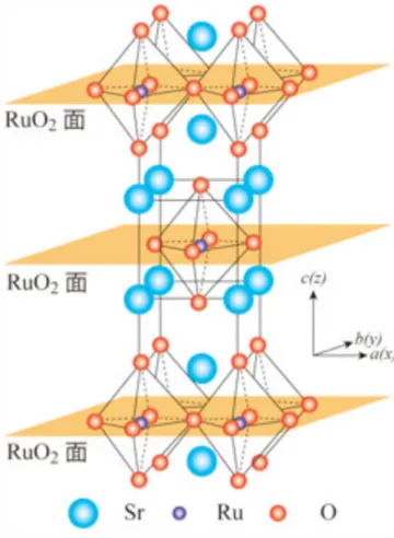
Sr2RuO4

1. Topological insulators

- Z2 bulk invariants

- Three-dimensional topological insulator

[picture courtesy S. Zhang et al.]

(3)

e.g.: Pf

✓ 0 z z 0

◆

= z

consider anti-symmetric “t-matrix”:

)

antisymmetry property:

) Pfaffian can be defined:

(Pf [!( _a)])²

= det [!( _a)]

[Kane Mele 05]

[Fu and Kane]

— denote gauge choices in the two EBZs

— TR-smooth gauge: _|_u⁽¹⁾_n ₍ _k)_⇥ ₌ _|_u⁽²⁾_n _(k)_⇥

|u⁽¹⁾_n (k) and |u⁽²⁾_n (k)

Bulk Z2 invariant as an obstruction to define a “TR-smooth gauge”:

t_mn(k) = ⌦

u_m(k) ⇥ u_n (k)↵

t^T(k) = t(k)

Pf [t(k)]

Zeroes of occur in  

isolated points, carry phase winding

2D topological insulator: First bulk Z2 invariant

Due to time-reversal symmetry:

(i) |Pf[t(k)]| = |Pf[t( k)]| ) zeros come in pairs

(ii) At TRI momenta ⇤_a we have |Pf[t(⇤_a)]| = 1 ) zeros cannot be brought to TRI momenta

Festk¨orperphysik II, Musterl¨osung 11.

Prof. M. Sigrist, WS05/06 ETH Z¨urich

we have

k_x k_y π/a − π/a (1)

majoranas

γ₁ = ψ + ψ^† (2)

γ₂ = −i !

ψ − ψ^†"

(3) and

ψ = γ₁ + iγ₂ (4)

ψ^† = γ₁ − iγ₂ (5)

and

γ_i² = 1 (6)

{γ_i, γ_j} = 2δ_ij (7)

mean field

γ_E^† ₌₀ = γ_E₌₀ (8)

⇒ γ_k^†_,E = γ₋_k_,−E (9) Ξ ψ₊k,+E = τ_xψ₋^∗ k,−E (10) Ξ² = +1 Ξ = τ_xK (11)

τ_x =

#0 1

1 0

$

(12) c^†c c^†c ⇒ ⟨c^†c^†⟩c c = ∆^∗c c (13) weak vs strong

|µ| < 4t (14)

n = 1 (15)

Lattice BdG Hamiltonian ˆ

m(k) = m(k)

|m(k)| m(k) :ˆ m(k)ˆ ∈ S² π₂(S²) = (16) H_BdG = (2t [cos k_x + cos k_y] − µ) τ_z + ∆₀ (τ_x sin k_x + τ_y sin k_y) = m(k) · τ (17)

m_x m_y m_z (18)

and time-reversal symmetry

Θ = e^+iπS^y^/^!K Θ² = −1 2e²/h Λ_i Λ₁ Λ₂ Λ₃ Λ₄ (1)

E₀ k_y (2)

2γ_C = solid angle swept out by ˆd(k) (3) H(k) = d(k) · σ dˆ (4)

n = i 2π

! "

Fd²k (5)

|u(k)⟩ → e^iφ^k |u(k)⟩ (6)

A → A + ∇^kφ^k (7)

F = ∇^k × A (8)

γ_C =

#

C

A · dk (9)

γ_C =

"

S

Fd²k (10)

=⇒ (11)

Bloch theorem

[T (R), H] = 0 k |ψ_n⟩ = eⁱ^kr |u_n(k)⟩ (12) (13) H(k) = e⁻ⁱ^krHe⁺ⁱ^kr (14) (15) H(k) |u_n(k)⟩ = E_n(k) |u_n(k)⟩ (16) we have

H(k) k_x k_y π/a − π/a k ∈ Brillouin Zone (17) majoranas

γ₁ = ψ + ψ^† (18)

γ₂ = −i $

ψ − ψ^†%

(19) and

ψ = γ₁ + iγ₂ (20)

ψ^† = γ₁ − iγ₂ (21)

E₀ k_y (2)

2γ_C = solid angle swept out by ˆd(k) (3)

H(k) = d(k) · σ dˆ (4)

n = i 2π

! "

Fd²k (5)

|u(k)⟩ → e^iφ^k |u(k)⟩ (6)

A → A + ∇^kφ^k (7)

F = ∇^k × A (8)

γ_C =

#

C

A · dk (9)

γ_C =

"

S

Fd²k (10)

=⇒ (11)

Bloch theorem

γ₁ = ψ + ψ^† (18)

γ₂ = −i $

ψ − ψ^†%

(19) and

ψ = γ₁ + iγ₂ (20)

ψ^† = γ₁ − iγ₂ (21)

E₀ k_y (2)

n = i 2π

! "

Fd²k (5)

|u(k)⟩ → e^iφ^k |u(k)⟩ (6)

A → A + ∇^kφ^k (7)

F = ∇^k × A (8)

γ_C =

#

C

A · dk (9)

γ_C =

"

S

Fd²k (10)

=⇒ (11)

Bloch theorem

[T (R), H] = 0 k |ψn⟩ = eⁱ^kr |un(k)⟩ (12) (13) H(k) = e⁻ⁱ^krHe⁺ⁱ^kr (14) (15) H(k) |un(k)⟩ = En(k) |un(k)⟩ (16) we have

γ₁ = ψ + ψ^† (18)

γ₂ = −i $

ψ − ψ^†%

(19) and

ψ = γ₁ + iγ₂ (20)

ψ^† = γ1 − iγ2 (21)

E₀ k_y (2)

n = i 2π

! "

Fd²k (5)

|u(k)⟩ → e^iφ^k |u(k)⟩ (6)

A → A + ∇^kφ^k (7)

F = ∇^k × A (8)

γ_C =

#

C

A · dk (9)

γ_C =

"

S

Fd²k (10)

=⇒ (11)

Bloch theorem

[T(R), H] = 0 k |ψ_n⟩ = eⁱ^kr |u_n(k)⟩ (12) (13) H(k) = e⁻ⁱ^krHe⁺ⁱ^kr (14) (15) H(k) |u_n(k)⟩ = E_n(k) |u_n(k)⟩ (16) we have

γ₁ = ψ + ψ^† (18)

γ₂ = −i $

ψ − ψ^†%

(19) and

ψ = γ₁ + iγ₂ (20)

ψ^† = γ₁ − iγ₂ (21)

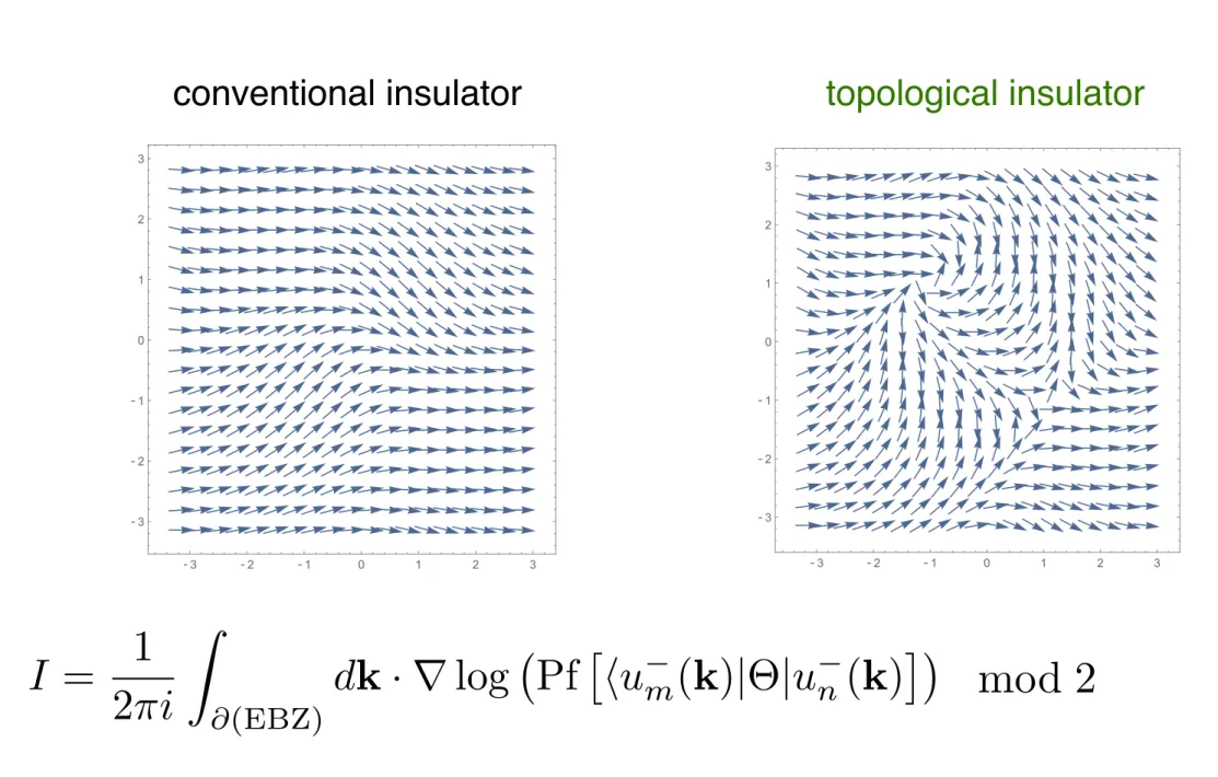
EBZ

(4)

conventional insulator topological insulator

Topological invariant = number or zeros of in EBZ modulo 2Pf [t(k)]

I = 1 2 i

Z

(EBZ)

dk · ⇥ log Pf ⇥

u_m(k)| |u_n (k)⇤

mod 2

It follows from bulk-boundary correspondence: edge Z2 invariant = bulk Z2 invariant

2D topological insulator: First bulk Z2 invariant

Figure 4: Gap glosing points for µ = 2, 0 and 2

The corresponding complex P(k) is plotted in Fig. 5. It can be seen that at µ = 1, there are two vortices in BZ.

Figure 5: complex field of P(k) at µ = 1, and 2.

Figure 4: Gap glosing points for µ = 2, 0 and 2

The corresponding complex P(k) is plotted in Fig. 5. It can be seen that at µ = 1, there are two vortices in BZ.

Figure 5: complex field of P(k) at µ = 1, and 2.

(5)

e.g.: Pf

✓ 0 z z 0

◆

= z

2D topological insulator: Second bulk Z2 invariant

consider unitary sewing matrix:

)

mn(k) = ⇥u_m( k)| |u_n (k)⇤

antisymmetry property: !^T (k) = !( k)

at TRI momenta: _a = _a ) !^T ( _a) = !( _a) is antisymmetric

) Pfaffian can be defined: Pf [!( _a)] ^{(Pf [!(} ^a^)])

2

= det [!( _a)]

Bulk Z₂ invariant ( = 0,1):⌫ ^{( 1) =}

Y4

a=1

Pf [!( _a)]

pdet [!( _a)] = ±1 (gauge invariant, but smooth

gauge needed)

[Kane Mele 05]

[Fu and Kane]

It follows from bulk-boundary correspondence: edge Z2 invariant = bulk Z2 invariant

— denote gauge choices in the two EBZs

— TR-smooth gauge: _|_u⁽¹⁾_n ₍ _k)_⇥ ₌ _|_u⁽²⁾_n _(k)_⇥

|u⁽¹⁾_n (k) and |u⁽²⁾_n (k)

Bulk Z2 invariant as an obstruction to define a “TR-smooth gauge”:

we have

k_x k_y π/a − π/a (1)

majoranas

γ₁ = ψ + ψ^† (2)

γ₂ = −i !

ψ − ψ^†"

(3) and

ψ = γ₁ + iγ₂ (4)

ψ^† = γ₁ − iγ₂ (5)

and

γ_i² = 1 (6)

{γ_i, γ_j} = 2δ_ij (7)

mean field

γ_E^† ₌₀ = γ_E₌₀ (8)

⇒ γ_k^†_,E = γ₋_k_,−E (9) Ξ ψ₊k,+E = τ_xψ₋^∗ k,−E (10) Ξ² = +1 Ξ = τ_xK (11)

τ_x =

#0 1

1 0

$

|µ| < 4t (14)

n = 1 (15)

m(k) = m(k)

|m(k)| mˆ (k) : mˆ (k) ∈ S² π₂(S²) = (16) H_BdG = (2t [cos k_x + cos k_y] − µ) τ_z + ∆₀ (τ_x sin k_x + τ_y sin k_y) = m(k) · τ (17)

m_x m_y m_z (18)

we have

k_x k_y π/a − π/a (1)

majoranas

γ₁ = ψ + ψ^† (2)

γ₂ = −i !

ψ − ψ^†"

(3) and

ψ = γ₁ + iγ₂ (4)

ψ^† = γ₁ − iγ₂ (5)

and

γ_i² = 1 (6)

{γ_i, γ_j} = 2δ_ij (7)

mean field

γ_E^† ₌₀ = γ_E₌₀ (8)

⇒ γk^†,E = γ₋k,−E (9) Ξ ψ₊k,+E = τ_xψ₋^∗ k,−E (10) Ξ² = +1 Ξ = τ_xK (11)

τ_x =

#0 1

1 0

$

|µ| < 4t (14)

n = 1 (15)

m(k) = m(k)

|m(k)| mˆ (k) : mˆ (k) ∈ S² π₂(S²) = (16) H_BdG = (2t [cos k_x + cos k_y] − µ) τ_z + ∆₀ (τ_x sin k_x + τ_y sin k_y) = m(k) · τ (17)

m_x m_y m_z (18)

E₀ k_y (2)

2γC = solid angle swept out by ˆd(k) (3) H(k) = d(k) · σ dˆ (4)

n = i 2π

! "

Fd²k (5)

|u(k)⟩ → e^iφ^k |u(k)⟩ (6)

A → A + ∇^kφ^k (7)

F = ∇^k × A (8)

γ_C =

#

C

A · dk (9)

γ_C =

"

S

Fd²k (10)

=⇒ (11)

Bloch theorem

[T(R), H] = 0 k |ψn⟩ = eⁱ^kr |un(k)⟩ (12) (13) H(k) = e⁻ⁱ^krHe⁺ⁱ^kr (14) (15) H(k) |u_n(k)⟩ = E_n(k) |u_n(k)⟩ (16) we have

γ₁ = ψ + ψ^† (18)

γ₂ = −i $

ψ − ψ^†%

(19) and

ψ = γ₁ + iγ₂ (20)

ψ^† = γ₁ − iγ₂ (21)

E₀ k_y (2)

H(k) = d(k) · σ dˆ (4)

n = i 2π

! "

Fd²k (5)

|u(k)⟩ → e^iφ^k |u(k)⟩ (6)

A → A + ∇^kφ^k (7)

F = ∇^k × A (8)

γ_C =

#

C

A · dk (9)

γ_C =

"

S

Fd²k (10)

=⇒ (11)

Bloch theorem

γ₁ = ψ + ψ^† (18)

γ₂ = −i $

ψ − ψ^†%

(19) and

ψ = γ₁ + iγ₂ (20)

ψ^† = γ₁ − iγ₂ (21)

E₀ k_y (2)

n = i 2π

! "

Fd²k (5)

|u(k)⟩ → e^iφ^k |u(k)⟩ (6)

A → A + ∇^kφ^k (7)

F = ∇^k × A (8)

γ_C =

#

C

A · dk (9)

γ_C =

"

S

Fd²k (10)

=⇒ (11)

Bloch theorem

γ₁ = ψ + ψ^† (18)

γ₂ = −i $

ψ − ψ^†%

(19) and

ψ = γ₁ + iγ₂ (20)

ψ^† = γ₁ − iγ₂ (21)

E₀ k_y (2)

H(k) = d(k) · σ dˆ (4)

n = i 2π

! "

Fd²k (5)

|u(k)⟩ → e^iφ^k |u(k)⟩ (6)

A → A + ∇^kφ^k (7)

F = ∇^k × A (8)

γ_C =

#

C

A · dk (9)

γ_C =

"

S

Fd²k (10)

=⇒ (11)

Bloch theorem

γ₁ = ψ + ψ^† (18)

γ₂ = −i $

ψ − ψ^†%

(19) and

ψ = γ₁ + iγ₂ (20)

ψ^† = γ₁ − iγ₂ (21)

EBZ