Bulk and Confinement Effects
Lisa Heße and Klaus Richter
Institut f¨ur Theoretische Physik, Universit¨at Regensburg, D-93040 Regensburg, Germany (Dated: April 29, 2014)
We consider the orbital magnetic properties of non-interacting charge carriers in graphene-based nanostructures in the low-energy regime. The magnetic response of such systems results both, from bulk contributions and from confinement effects that can be particularly strong in ballistic quantum dots. First we provide a comprehensive study of the magnetic susceptibility χof bulk graphene in a magnetic field for the different regimes arising from the relative magnitudes of the energy scales involved,i.e. temperature, Landau level spacing and chemical potential. We show that for finite temperature or chemical potential,χis not divergent although the diamagnetic contribution χ0 from the filled valance band exhibits the well-known −B−1/2 dependence. We further derive oscillatory modulations ofχ, corresponding to de Haas-van Alphen oscillations of conventional two- dimensional electron gases. These oscillations can be large in graphene, thereby compensating the diamagnetic contributionχ0 and yielding a net paramagnetic susceptibility for certain energy and magnetic field regimes. Second, we predict and analyze corresponding strong, confinement-induced susceptibility oscillations in graphene-based quantum dots with amplitudes distinctly exceeding the corresponding bulk susceptibility. Within a semiclassical approach we derive generic expressions for orbital magnetism of graphene quantum dots with regular classical dynamics. Graphene-specific features can be traced back to pseudospin interference along the underlying periodic orbits. We demonstrate the quality of the semiclassical approximation by comparison with quantum mechanical results for two exemplary mesoscopic systems, a graphene disk with infinite mass-type edges and a rectangular graphene structure with armchair and zigzag edges, using numerical tight-binding calculations in the latter case.
PACS numbers: 73.22.Pr, 73.20.At, 03.65.Sq, 75.20.-g, 05.30.Fk
I. INTRODUCTION
Since the seminal work of Landau1 it is known that a conventional free electron gas exihbits a weak dia- magnetic orbital magnetic response. In two dimensions (2d) and at low magnetic field, its magnetic susceptibil- ity χ is just a constant, i.e. independent of Fermi en- ergy and B-field. For Dirac fermions in 2d, e.g. charge cariers in graphene close to the charge neutrality point, the situation is different: As McClure showed nearly 50 years ago2, a non-interacting 2d system of massless Dirac fermions features a Curie-type 1/kBT behavior3 at finite temperatureT that merges, for vanishing tem- perature, into a peculiar dependence on the chemical potential2,4–11 : χ∼δ(µ), i.e. a magnetic response that is divergent in the undoped limit and otherwise zero.
In this work we pose the question how orbital mag- netism in graphene-based nano- and mesoscale systems is altered through the presence of the confinement. Similar questions had been intensively discussed in the early nin- tees for small disordered metallic rings12, quasi ballistic micron-sized rings13 and square cavities14 based on con- ventional 2d electron systems. The magnetic response of (ensembles of) these mesoscopic systems, namely the ob- served persistent current in the rings and the susceptibil- ity of the cavities, turned out to exceed the bulk Landau diamagnetism by one to two orders of magnitude. These original experimental findings triggered broad theoretical activities (for reviews see15–17) investigating in particular also the role of non-interacting versus interacting contri-
butions to the orbital magnetism. While twenty years ago further progress in the field had been hindered by exper- imental limitations, recent new high-precision cantilever magnetization (persistent current) measurements of en- sembles of rings proved18 the feasibility to reliably mea- sure orbital magnetism of nanoscale objects. The results of these recent experiments are essentially in line with earlier theory based on non-interacting systems19. Given the peculiar orbital magnetic behavior of bulk graphene, and in view of the above mentioned possibility to observe confinement-enhanced magnetism in nanostructures18, it hence is of interest to explore also orbital magnetism in graphene nanostructures, a topic that has been barely addressed in the literature.
Here, we employ a trajectory-based semiclassical path integral formalism to compute the orbital magnetic sus- ceptibility. As recently shown, such an approach is suit- able for the quantitative description and interpretation of the density of states20and conductance21of graphene- based cavities. This approach allows for the incorpora- tion of graphene-specific boundary effects (zigzag, arm- chair and infinite mass). The confinement geometry and the type of edge is then encoded in the amplitudes and phases of paths (hitting the boundaries) that enter into the respective semiclassical trace formulae. We com- bine this approach with an earlier semiclassical treatment of orbital magnetism in conventional ballistic electron cavities16,22. We show that the susceptibility of graphene cavities of linear system size R exhibits confinement- induced oscillations in kFR where kF is the Fermi mo-
arXiv:1403.3688v3 [cond-mat.mes-hall] 28 Apr 2014
mentum. For integrable geometries and at low temper- atures their amplitude is parametrically larger by a fac- tor of√
kFRthan the corresponding bulk susceptibility.
However, graphene cavities additionally carry features of bulk graphene. Hence, in the first part of the paper we include a comprehensive discussion of graphene bulk or- bital magnetism. While a number of previous works ad- dressed various parameter regimes separately we aim at a systematic presentation of the various bulk regimes.
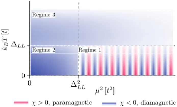
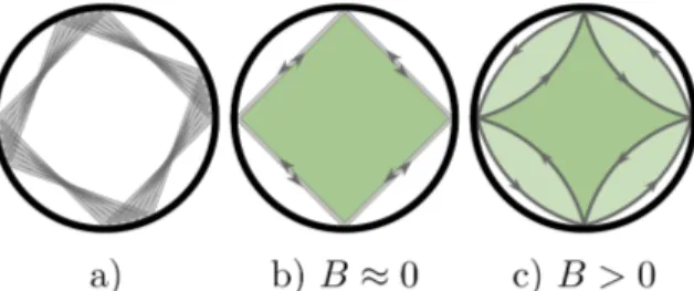
FIG. 1: Rough schematic overview of the orbital magnetic behaviour of graphene in a perpendicular field for the en- ergy regimes studied in Subsec. III D. Here µ is the chemi- cal potential, kBT the thermal energy and ∆LL ∝√
B rep- resents the Landau level spacing. Blue (red) regions refer to parameter regimes where graphene shows diamagnetism (paramganetism). The colour intensity roughly indicates the strength of the magnetic response. The magnetic susceptibil- ityχis diamagnetic in allmost all areas except the de Haas- van Alphen regime, µ > ∆LL > kBT, with susceptibility
oscillations ofχbeing linear inµ2 (and 1/B).
This is simplistically sketched in Fig. 1. It shows an overall diamagnetic behavior up to the energy re- gion governed by de Haas-van Alphen oscillations23–27for kBT <∆LL < µ, with ∆LL proportional to the Landau level spacing. However, the diamagnetic regions exhibit interesting parametrical dependences that we will derive and review. For instance, the afore mentioned divergent behavior ofχ at T= 0 is smoothed out if kBT is bigger than the mean level spacing.
The paper is organized as follows: After summarizing the necessary thermodynamic formalism in Sec. II, we first give a comprehensive account of bulk magentism in graphene in Sec. III, addressing the various parameter regimes mentioned above. This also involves introducing our numerical approach and our scheme to extract bulk results from the numerics performed for finite systems.
In the other main Sec. IV we consider in detail finite-size effects in the orbital magnetic response of nanostructued graphene. There we generalize the existing semiclassical approaches to quantitatively describe and interprete os- cillatory effects in the susceptibility. These semiclassical predictions are compared to corresponding quantum cal- culations for disc-like and rectangluar geometries. We fo- cus on integrable structures since chaotic or diffusive ge-
ometries are expected to exhibit a parametically weaker magnetic response.
II. BASIC THERMODYNAMIC QUANTITIES In order to investigate the orbital magnetic properties of a quasi-two dimensional solid in general, it is conve- nient to start from the total grand potential in the pres- ence of a perpendicular magnetic field of strengthB,
Ω(µ, B) =−1 β
Z∞
−∞
dE ρ(E, B) lnh
1 + e−β(E−µ)i , (1)
where 1/β=kBT denotes the thermal energy. The chemical potential µ is assumed to be B-independent.
The total density of states28 (DOS), ρ(E, B) = ρv(E, B) + ρc(E, B), comprises conduction and va- lence band states simultaneously as well as the field- dependence of the energy spectrum of the solid. Defin- ing Ev/c as the energy of the band edge of the va- lence/conduction band, the corresponding densities of states fullfilρv/c(E, B) = 0,∀E≷Ev/c, even for a van- ishing energy gap Eg=Ec−Ev = 0 as in the case of graphene. Without loss of generality,µ is chosen to be larger thanEv. Due to the properties of the total DOS, the grand potential can be decomposed as Ω = Ωv+ Ωc, where
Ωv(µ, B) =−1 β
Ev
Z
−∞
dE ρv(E, B) lnh
1 + e−β(E−µ)i , (2)
Ωc(µ, B) =−1 β
Z∞
Ec
dE ρc(E, B) lnh
1 + e−β(E−µ)i . (3)
Equation (3) contains the contribution to Ω from elec- trons in the conduction band for Fermi energiesµ > Ev or thermal excitation. In the limit T → 0 only states with energyEc ≤E≤µare occupied. In view of
− lim
β→∞
1
β ln 1 + e−βx
=x θ(−x), (4) and taking the limitT→0 in Eq. (2), yields the contri- bution to Ω from the completely filled valence band:
Ω0(µ, B) =
Ev
Z
−∞
dE ρv(E, B)(E−µ). (5)
In general, the integral (5) can diverge, if the particular model assumes a valence band without lower boundary.
As we will discuss in Subsec. III C for bulk graphene in the low energy approximation, Ω0 can be decomposed into aB-field-dependent and a divergent part, which does
not include any field-dependence and therefore has no effect on the magnetic properties.
By pulling a factor exp [−β(E−µ)] out of the loga- rithm in Eq. (2) Ωv can be represented as
Ωv(µ, B) = Ω0(µ, B)
− 1 β
Ev
Z
−∞
dE ρv(E, B) lnh
1 + eβ(E−µ)i .(6) The second term in Eq. (6) contains a similar contribu- tion to Ω as Ωc corresponding to electron vacancies at finite temperature. As a first conclusion, Ω can be de- composed into theT-independent part Ω0, coming from the filled part of the valence band, and a contribution
ΩT(µ, B) = Ω(µ, B)−Ω0(µ, B) (7)
=−1 β
Z∞
−∞
dE n
ρv(E, B) lnh
1 + eβ(E−µ)i +ρc(E, B) lnh
1 + e−β(E−µ)io (8)
due to excited electrons in the conduction band and holes in the valence band. Within the relevant temperature range the integral (8) converges fast due to the exponen- tial decay of the integrand at both integration limits.
The total magnetic susceptibility is defined as χ(µ, B) =−µ0
A
∂2Ω(µ, B)
∂B2
T,µ
. (9)
In view of Eq. (7), it can be decomposed into
χ(µ, B) = χ0(µ, B) +χT(µ, B), (10) with
χx(µ, B) =−µ0
A
∂2Ωx(µ, B)
∂B2
T,µ
, x = 0, T. (11) Here, A denotes the area of the system and µ0 is the vacuum permeability. As will be shown in Subsec. III C for bulk graphene, χ0, which is of similar origin as the Landau susceptibility1,16 of non-relativistic electron gases, represents a smooth, diamagnetic contribution
∝ 1/√
B 3,5,11,26 to the total susceptibility. Contrarily, χT in Eq. (10) can yield an oscillatory contribution toχ for certain energy regimes. In bulk systems this oscilla- tory behavior refers to the de Haas-van Alphen effect23,29, whereas in finite systems additional modulations inχoc- cur as signatures of the confinement, see Sec. IV.
III. BULK ORBITAL SUSCEPTIBILITY A. Spectral properties of Landau quantized charge
carriers with linear dispersion
In this section the orbital magnetic properties of bulk graphene in the energy range of linear dispersion are dis-
cussed. The graphene sheet is assumed to lie in the x- y-plane perpendicular to an external, homogeneous B- field. Then the energies of the charge carriers are Landau quantized1. The Landau levels of massless Dirac-Weyl particles in 2D describing bulk graphene read30–32
En= sgn(n)
√2~vF lB
p|n|, (12) with n∈Z. Here, lB=p
φ0/(2πB) denotes the mag- netic length with the magnetic flux quantumφ0=h/e.
Every Landau level En has a twofold spin degeneracy gs and valley degeneracy gv as well as a ϕ=φ/φ0- fold degeneracy (φ=BA) which can be, e.g., deduced from phase space arguments23,33 and Bohr-Sommerfeld quantization34 of the corresponding cyclotron orbits.
Thus the orbital degeneracy in graphene is identical to that of Landau levels of ordinary 2D electron gases1, n= (~/m∗)eB(n+ 1/2), with effective mass m∗ and n∈N0. In this case the lowest Landau level has the finite value0= (~/m∗)eB/2 while for grapheneE0= 0 attains zero and lies precisely at the touching point of conduction and valence band. In the presence of a mag- netic field conduction and valence band states occupy the zeroth Landau level equally leading to an increase of the total energy of the filled valence band. Thus the contributionχ0 from the filled valence band is expected to be diamagnetic as discussed in detail in Subsec. III C.
Whether the total susceptibilityχ, Eqs. (9, 10), is para- or diamagnetic depends on the contributionχT of excited electrons and holes in the particular energy regime.
The single-particle DOS of bulk graphene, ρ(E, B) =g ϕ
∞
X
n=−∞
δ(E−En(B)), (13) can be decomposed into a smooth and an oscillatory part with respect to E and B. By means of Poisson summation35of the Landau index none obtains
ρ(E, B) =C|E|
"
1 + 2
∞
X
m=1
cos πm E lB
~vF 2!#
(14)
= ¯ρ(E) +ρosc(E, B) (15) with C=gA/[2π(~vF)2] and g=gsgv. Note that each term in Eqs. (14, 15) and thereby the total DOS reflects particle-hole symmetry, i.e.ρ(E, B) =ρ(−E, B), due to the nearest neighbor hopping approximation underly- ing the effective Dirac hamiltonian. The smooth part
¯
ρ(E) =C|E|isB-independent and identical to the bulk DOS of the field free system36. Hence the entire con- tribution toχarises from the oscillatory partρosc(E, B) that can be rewritten as
ρosc(E, B) =g ϕ
∞
X
n=1
[δ(E−En(B)) +δ(E+En(B))]
+g ϕ δ(E)−C|E|. (16)
This represention clearly indicates that the orbital mag- netism arises only from Landau levels withn 6= 0. The zeroth Landau level leads to aϕ-linear contribution to Ω and thus does not contribute toχ. As for the DOS the re- lated thermodynamic potentials can be decomposed into Ω(µ, B) = ¯Ω(µ) + ˜Ω(µ, B). (17) Each term in Eq. (17) can be further split as shown in Eqs. (7, 10), i.e. X=X0+XT, where X = ¯Ω,Ω. Note˜ that ¯Ω arises directly from the field independent bulk DOS ¯ρ(E), and hence χ∝∂2Ω/ ∂B2
=∂2Ω/ ∂B˜ 2 . We will show below that though ˜Ω arises from the oscil- latory part of the DOS, it yields not only an oscillatory but also a smooth contribution to the susceptibility.
B. Comparability of numerical results with analytical bulk DOS calculations
The comparison between the analytical results for bulk graphene, to be discussed in Subsec. III C and III D, with the numerical tight-binding data of confined graphene quantum dots will demonstrate the importance of bulk effects in finite structures. Moreover, vice versa, we will employ the numerical calculations, restricted to finite gemetries, to confirm the results from the effective bulk theory based on the Dirac equation. For such a com- parison we need to extract the bulk contribution from the numerical results in an appropriate way as discussed below.
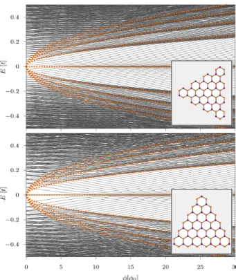
The finite systems considered have an equilateral tri- angular geometry with either pure armchair or zigzag boundaries. This particular choice of geometry enables also a distinct analysis of edge effects due to zigzag boundaries. Each system has mesoscopic dimensions, i.e. the triangle side lengths are L ≈100a, where a is the graphene lattice constant, such that the region of linear dispersion contains enough energy levels to re- quire good comparability with the theory. The eigenen- ergies of the triangles are calculated within tight-binding approximation37,38 including only nearest neighbor hop- ping t and using the Lanczos algorithm39,40. Figure 2 shows the resulting energy spectrum for conduction and valence band energies |E| ≤0.55t as a function of the normalized magnetic flux φ/φ0. One can clearly see the condensation of the eigenenergies into Landau levels41,42for fluxes φ > 5φ0. This is the regime where bulk effects should be distinctly observable in the finite systems.
In Subsec. III C we calculate the contributionχ0from the valence band in Dirac approximation, which corre- sponds to the Landau susceptibility of electron gases.
Therefore we assume an unbounded valence band with linear dispersion which does not reflect the real band structure of graphene further away from the Dirac point.
For this reason,χ0is not accessible within tight-binding approximation even if one would go to very large sys- tem sizes. Thus the comparison of the analytic theory
FIG. 2: (Color online) Energy spectrum of triangular quan- tum dots with armchair edge (upper panel) and zigzag edge (lower panel) as a function of the normalized magnetic flux through each system. The dashed green lines refer to the lowest Landau energiesEn. In the case of zigzag geometry the zigzag edge states clearly appear close toE≈0 and con- tribute to the zeroth Landau level. Insets: Sketch of the geometries, the actual systems considered are much larger:
L '100a.
with numerical data for the quantum dots is restricted to the temperature dependent part of ˜Ω andχ, respec- tively, where only the energy levels close to the Fermi level contribute.
As one can deduce from Fig. 2 the mean level spacings
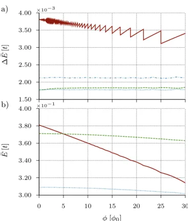
∆ ¯E(ac,zz) of the finite systems differ from the mean Lan- dau level spacing ∆ ¯E(bulk)of the bulk system. In Fig. 3a) we compare explicitly ∆ ¯E(x) (x = ac, zz, bulk), calcu- lated from the first 600 electronic states for each case, as a function of the normalized magnetic flux. When dealing with thermodynamic potentials and related observables, finite temperatureT, encoded in the Fermi-Dirac statis- tics, implies an effective broadening 1/β of each energy level as can be seen from Eq. (8). For an appropriate comparison of the Dirac-type bulk theory with the tight- binding results for the finite-size structures the thermal energies chosen should obey
β(bulk)∆ ¯E(bulk)(φ)≈β(x)∆ ¯E(x)(φ), x = ac,zz. (18) To get reliable values from this expression the edge states are not considered in the case of the zigzag system since they lead to underestimating the mean level spacing.
To compare the properties of the bulk system with those of the quantum dots for finite magnetic flux it
is necessary to average Eq. (18) over the flux interval considered. The resulting level spacings averaged over φ ∈ [0,30φ0] can be read off from Table I. The above procedure, providing an adequate comparison between all three systems, refers to the entire thermodynamic potentials and related properties. Independently, the individual energy levels for each of the considered sys- tems can be written as Ei(x) = ¯E(x) +δEi(x), where E¯(x)= 1/N PN
i=1Ei(x) denotes the mean energy of the N valence band states considered. Figure 3b) shows the flux dependence of ¯E(x) for each system averaged over the lowestN= 600 electron states. In all three cases the mean energies are of the same order of magnitude. Due to the contribution of edge states, ¯Eac>E¯zz.
1.50 2.00 2.50 3.00 3.50
a) 4.00 ×10⁻³
∆¯E[t]
3.00 3.20 3.40 3.60 3.80 4.00
0 5 10 15 20 25 30
φ[φ0]
b) ×10−1
¯E[t]
FIG. 3: (Color online) a) Comparison of the mean level spac- ing (in units of hopping energy t) of the lowest 600 electron states of the two triangluar quantum dots, see Fig. 2, with the Dirac model for bulk graphene (red solid line) calculated from Eq. (12) as a function of the magnetic flux. The blue dotted (dashed-dotted) line represents the mean level spacing of the zigzag system with (without) considering edge states.
Due to the edge states ∆E is smaller than in the armchair system (green dashed line). b) Mean energy of the lowest 600 electronic energies as a function of the magnetic flux. The full (red), dotted (blue) and dahed (green) lines correspond
to the bulk, zigzag and armchair system, respectively.
x bulk armchair zigzag
h∆ ¯E(x)iφ 10−3t
3.514 1.828 2.124 (1.780) hE¯(x)iφ [t] 0.349 0.368 0.306
TABLE I: Flux average of the mean energy hE¯(x)iφ and mean level spacingh∆ ¯E(x)iφfor the first 600 electron states of bulk graphene, an armchair and a zigzag triangular quantum dot, same as Fig. 2. The considered flux interval amounts to [0,30φ0]. The number in parenthesis comprises the edge
states.
The grand potential for each system reads Ω(x)(µ, B) =−1
β X
i
ln
1 + e−β
E¯(x)+δEi(x)−µ . (19) The properties of the exponential function and the logarithm yield a rough scaling behavior of Ω(ac,zz)/Ω(bulk)≈γ(ac,zz) for each system reflecting in first approximation
βac,zzE¯(ac,zz)−βbulkE¯(bulk)≷0. (20) Resulting differences in the absolute value of Ω and χ, respectively, for fixed µ and ϕ can be approximately compensated by rescaling the bulk value with the fac- torγ(ac,zz). The factorsγ(ac,zz) were obtained by fitting using the Levenberg-Marquardt43algorithm.
As a consequence of ¯Eac>E¯zz, Fig. 3(b), and Eq. (19) we expect the susceptibility contributionχT for a zigzag triangular quantum dot to be smaller than for the cor- responding armchair system at same temperature corre- sponding to Eq. (20). This behavior is also confirmed in Ref. [44], where the orbital magnetic properties of hexag- onal and triangular graphene nanostructures are numer- ically studied within tight-binding approximation.
C. Susceptibility contribution from filled valence band
As discussed in Subsec. III A, the susceptibility contri- bution χT from the filled valence band, Eq. (5), can be evaluated from Eq. (8) by using only the field-dependent part of the DOS,ρosc(E, B):
Ω˜0(µ, B) =
0
Z
−∞
dE ρosc(E, B)(E−µ) (21)
=−2C
∞
X
m=1
Re
"
η→0lim Z∞
0
dE E2+µE
×e−
η−iπm
lB
~vF
2 E2#
.
(22)
Solving this integral and taking the limitη→0 yields Ω˜0(B) =K
2 ϕ3/2
∞
X
m=1
1 m3/2 =K
2 ϕ3/2ζ 3
2
, (23) where all prefactors are absorbed in the constant
K= 4√ π C
~vF
√A 3
= 2g ~vF
√Aπ. (24) Indeed, Ω0and thereby the corresponding susceptibility
χ0(B) =−µ0g φ20 ~vF
rA π
3ζ 32 4
√1
ϕ∝ − 1
√
B (25)
are independent of the chemical potential. χ0(B) is diamagnetic because the grand potential of the valence band, ¯Ω0+ ˜Ω0(B), increases in the presence of a per- pendicular magnetic field, i.e. ˜Ω0(B)>Ω˜0(0). The sus- ceptibility χ0 diverges as 1/√
B implying that small variations of the flux cause huge changes in the mag- netization of bulk graphene in the low-field regime.
The scaling behavior (25) of χ0 was first discovered by McClure in 1956 within his studies of the diamag- netic properties of graphite2 and confirmed by various research groups3,5,11,26,45 for monolayer graphene. In Sec. III D we show that this singularity of χ0, however, need not lead to a divergence of the total susceptibility χ=χ0+χT.
In the case of a bulk 2DEG the quantity corresponding toχ0is the Landau susceptibility16
χL=−µ0gsπ 6
~2
φ20m∗. (26) It is also independent ofµbut moreover does not depend onB. To estimate the relative strength of graphene dia- magnetism we consider the ratioχ0/χL which reads
χ0(B)
χL ≈0.2 m∗ me−
sA
ϕ nm−1. (27) To give an explicit example, consider GaAs (m∗= 0.067me−) and a graphene flake with a typ- ical length L/lB1, such that bulk effects dominate over finite-size signatures in χ. Choosing typical values φ=φ0 and A ≈1002nm2, Eq. (27) yieldsχ0≈χL, i.e.
the diamagnetic contribution from the valence band in graphene is comparable to the Landau susceptibility of a 2DEG for a magnetic field ofB≈0.5 T.
D. Susceptibility contribution from thermally excited charge carriers
To investigate the contribution toχfrom excited elec- trons and holes we start from Eq. (8) considering only the
field-dependent partρosc(E, B) of the DOS in Eq. (14):
Ω˜T(µ, B) =−1 β
Z∞
−∞
dE ρosc(E, B) (28)
×n
θ(−E) lnh
1 + eβ(E−µ)i
+θ(E) lnh
1 + e−β(E−µ)io . Due to the integration over energy and the temperature dependence of ˜ΩT the corresponding susceptibility χT can contain a smooth as well as an oscillatory part, which is directly accessible within the semiclassical description of finite-size contributions toχ as shown in Sec. IV.
For the following considerations it is useful to integrate Eq. (28) twice by parts yielding
Ω˜T(µ, B) = Z∞
−∞
dEN(E, B)f0(E−µ), (29)
with the integral over particle number fluctuations,
N(E, B) =
E
Z
0
dE0
E0
Z
0
dE00ρosc(E, B) (30)
=Kϕ3/2
∞
X
m=1
S√
πm|E~v|lB
F
m3/2 . (31) Here, S(x) =p
2/πRx
0 dt sin t2
is the Fresnel integral46 andKis defined by Eq. (24). In Eq. (29)
f0(x) =−β 4sech2
β 2x
β→∞
−−−−→ −δ(x) (32) denotes the derivative of the Fermi distribution function f(x) = [1 + exp (β x)]−1. We rewrite Eq. (29) as
Ω˜T(µ, B) =Kϕ3/2
∞
X
m=1
ωm,T(µ, B)
m3/2 , (33) whereωm,T is defined as the energy integral
ωm,T(µ, B) = Z∞
−∞
dES √
πm|E|lB
~vF
f0(E−µ). (34)
Since the integral (34) cannot generally be solved ana- lytically, it is convenient to discuss separately different regimes defined through the ratios between the relevant length scales entering the problem, namely the magnetic length lB, the Fermi wavelength λF =~vF/µ, and the thermal wavelengthλT =~vFβ. For the sake of simplic- ity we define the two dimensionless parameters
α= λF
lB ∝ ∆LL
µ , γ=λT
lB ∝ ∆LL
kBT, (35) where ∆LL∝√
B denotes the energy spacing between adjacent Landau levels.
1. Regime: γ >1> α
In this parameter range the Landau level spacing is larger than or comparable to the thermal energy, but smaller than the chemical potential. The resulting tem- perature dependent contribution to Ω is therefore ex- pected to show an oscillatory modulation as a function of µ or ϕ known as de Haas-van Alphen effect in elec- tron gases23–25. Moreover we will show that the 1/√
B singularity in Eq. (25) is cancelled. Hence it is useful to decompose the Fresnel integral in Eq. (34) into its smooth and oscillatory part, i.e. sgn(x) S(x) = 1/2 + ˜S(x). The function ˜S(x) oscillates around zero and can be written in terms of the hypergeometric function U(1/2; 1/2,−ix2) or its integral representation as shown in App. A,
S(x) =˜ − 1
√2πIm
Z∞
0
du e−(u−i)x2
√π u(u−i)
. (36) Then the energy integral (34) reads
ωm,T =−1 2 +
Z∞
−∞
dES˜ √
πm|E| lB
~vF
f0(E−µ). (37)
Note that the remaining integral directly leads to the B field-dependent part of the total grand potential, Ω = ˜˜ Ω0+ ˜ΩT, since the first term in Eq. (37) exactly can- cels with ˜Ω0, Eq. (28), after inserting it into Eq. (33).
Then ˜Ω can be cast into the form Ω(µ, B) =˜
∞
X
m=1
Kϕ3/2
√
2π m3Im
Z∞
0
duYT(µ, B, u)
√π u(u−i)
, (38) with
YT(µ, B, u) = Z∞
−∞
dE f0(E−µ) e−(u−i)πm
E lB
~vF
2
. (39)
As shown in App. A of Ref. [16] for a similar situation, YT(µ, B, u)≈Y0(µ, B, u) RT[φ0(µ, B, u)], (40) where the temperature damping factor RT is defined as
RT[φ0(µ, B, u)] =
π
βφ0(µ, B, u) sinhh
π
βφ0(µ, B, u)i
β→∞
−−−−→1 (41)
and results from the derivative of the Fermi-Dirac distri- bution and φ0(µ, B, u) =∂φ(E, B, u)/(∂E)|E=µ. From Eqs. (40, 41) follows
YT(µ, B, u)≈e−(u−i)πm/α2RT
β2πm αγ
, (42)
so the field-dependent part of Ω finally reads Ω(µ, B)˜ ≈K
∞
X
m=1
ϕ3/2 m3/2
˜S √
π m α
RT
β2πm
αγ
. (43) Compared to the rapid magneto oscillations of ˜S, the factor RT only slowly varies on the relevant scales so that its magnetic field derivatives can be neglected in the calculation of the total magnetic susceptibility:
χ(µ, B) =−µ0g φ20 ~vF3√
A 2π
∞
X
m=1
RT β2πmαγ m3/2
J√ πm α
√ϕ (44)
=χ0(B)× 2
√πζ 32
∞
X
m=1
RT
β2πmαγ m3/2 J
√ πm α
, (45) with χ0(B) defined in Eq. (25). At finite temperatures the sum in Eq. (45) is exponentially damped due to RT, ensuring convergence of the corresponding expression.
The function J(x) is defined as J(x) = ˜S (x) +
r2 πx
sin x2
−2x2
3 cos x2
, (46) yieldingµ2- as well as 1/φ-periodic oscillations ofχ, re- spectively χT =χ−χ0, which can be extracted from Eq. (45) and Eq. (25). This becomes more obvious by transforming the expression (46) for J(x) into
J(x) =−cos x2
√2π
Σ1 x2 +4
3x3
−sin x2
√2π
Σ2 x2
−2x . (47) by defining Σ1/2(x2) = Im/Re[exp(iπ/4) U(1/2; 1/2;−ix2)]
and rewriting ˜S(x), Eq. (36). For the magnetization of bulk graphene an expression similar to Eq. (45) is derived in Ref. [26] considering additionally a band gap and impurity scattering, whereas in Ref. [27] the effect of an additional in-plane electric field is studied.
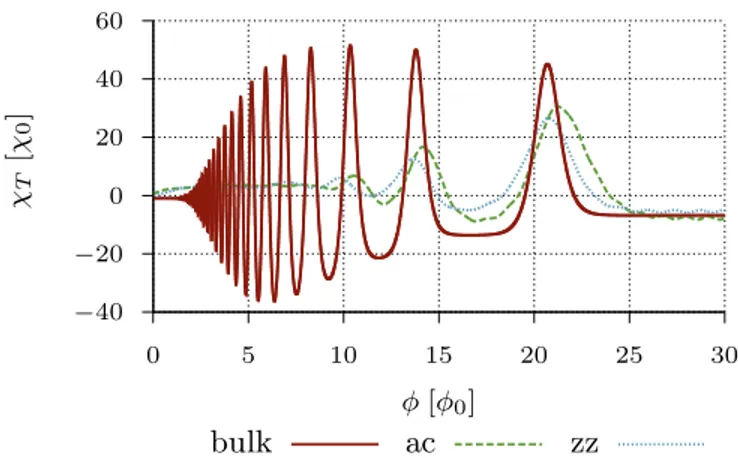
In Fig. 4 the oscillatory behavior of χT is demon- strated. In panel a) χT exhibits equidistant extrema when plottet as a function of µ2 at φ= 15φ0. Panel b) shows the 1/φ-periodicity of χT at µ= 0.3t. In both cases the thermal energy is chosen such that 1/β(bulk)≈3·10−3t. The amplitude of the χT oscilla- tions is about one order of magnitude larger than |χ0|, implying that the full orbital susceptibilityχof graphene oscillates between strong diamagnetic but also paramag- netic behavior as a function ofµand B, respectively.
In Fig. 5a) we show the numerically calculated sus- ceptibility contributionχT for a triangular armchair and zigzag quantum dot for the same value of the mag- netic flux as in Fig. 4a), i.e. φ = 15φ0. The thermal energies are chosen as 1/β(ac,zz)≈1·10−3t to satisfy relation (18). The levels of the finite systems are then
−90
−60
−30 0 30 60 90 120
0 0.125 0.25
EF2[t2] a)
χT[χ0]
−8
−4 0 4 8
0 0.2 0.4 0.6
1/φ[1/φ0] b)
FIG. 4: Susceptibility contributionχT for bulk graphene cal- culated from Eqs. (44, 45) at 1/β(bulk)≈3·10−3t. a) χT
shown as a function ofµ2 for fixedφ= 15φ0. b)χT plotted as a function of the inverse magnetic flux for fixedµ= 0.3t.
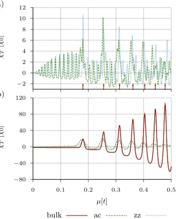
well resolved leading to extra peaks with smaller ampli- tude inbetween those caused by level clustering in the vicinity of Landau levels (see Fig. 2). The latter are in- dicated by red arrows in Fig. 5a) and coincide with the maxima in χT of the bulk system. These extra peaks are signatures of the confinement of the system and not captured within the bulk theory. Similar signatures are numerically observed in Ref. [44] for triangular but also hexagonal graphene quantum dots. In Sec. IV we will show how one can interprete these finite-size signatures within a semiclassical approach using periodic orbit the- ory. The amplitudes of the susceptibility oscillations of the quantum dots exceed the contribution χ0 from the filled valence band as well, implying that for certain ranges ofφandµthe total orbital magnetic susceptibil- ity can become paramagnetic. By raising the thermal en- ergy to 1/β(ac,zz)≈5·10−3t the finite-size features are smeared out and only extrema at the positions of the Landau levels survive as Fig. 5b) demonstrates.
Figure 6 compares the susceptibility contribution χT of the triangular quantum dots with the bulk system as a function ofφatµ= 0.3tand 1/β(bulk)≈3·10−3t, re- spectively 1/β(ac,zz)= 5·10−3t, such that finize-size ef- fects are smeared out. For flux valuesφ&10φ0the peak positions coincide very well. This corresponds to the spectral regime of the finite systems (see Fig 2) where the levels cluster in the vicinity of Landau levels and the influence of the boundaries becomes negligible.
2. Regime: α, γ >1
When the thermal energy and chemical potential are comparable to or smaller than the Landau level spacing the temperature dependent part of the susceptibility is expected to vanish3. If the magnetic field is tuned to very high values such that α, γ1 the degeneracy of each
−2 0 2 4 6 8 10
a) 12
χT[χ0]
−80
−40 0 40 80 120
0 0.1 0.2 0.3 0.4 0.5
µ[t]
b)
χT[χ0]
bulk ac zz
FIG. 5: Oscillatory susceptibility contributionχT for trian- gular graphene cavities as a function of the chemical poten- tial at φ= 15φ0. a) χT for armchair (green dashed) and zigzag (blue dotted) confinement with side lengthL ≈100a at 1/β(ac,zz)≈10−3t. The red arrows indicate the peak positions in the case of bulk graphene where only Lan- dau levels exist. b) Comparison of χT of the finite sys- tems (dashed and dotted) at a slightly higher thermal en- ergy 1/β(ac,zz)= 5·10−3twith the corresponding bulk result
(solid) at 1/β(bulk)≈3·10−3t.
Landau level rises accordingly, and all occupied states condense into the first or even to the zeroth levelE0. This yields a contribution to the temperature dependent part of the total grand potential ΩT linear inBas mentioned in Sec. III A. In order to calculate χT from Eq. (28) it is useful to apply the representation (16) forρosc. Then it is sufficient to consider only the sum over the Landau indices since the other terms do not contribute toχ. To this end we write
Ω˜T(µ, B) = ˆΩT(µ, B)−gϕ β
X
s=±1
∞
X
n=1
ln
1 + e−√2nγ+sαγ (48) where theB-linear term
ΩˆT(µ, B) =−g 2
ϕ β
X
s=±1
ln
1 + esγα
−Ω¯T(µ) (49)
−40
−20 0 20 40 60
0 5 10 15 20 25 30
φ[φ0] χT[χ0]
bulk ac zz
FIG. 6: Susceptibility contribution χT as a function of φ (for same triangular quantum dots as in Fig. 5) forµ= 0.3t, 1/β(bulk)≈3·10−3tand 1/β(ac,zz)= 5·10−3t.
The maxima coincide well with the bulk case for φ&10φ0, i.e. the flux range where the bulk theory is applicable to the
spectra of the finite quantum dots (see Fig. 2).
does not contribute to χT. Ω¯T, defined through Eqs. (7,15) is only based on the average DOS ¯ρ=C|E|.
In order to get an appropriate expression for ˜ΩT in this parameter range we Taylor expand the logarithm and the exponential function in Eq. (48) using the condition γ >1. Resumming the resulting triple infinite sums yields
Ω˜T(µ, B)≈ΩˆT(µ, B)−gϕ β
X
s±1
ln
1 + e−√2γ+sαγ , (50) as shown in App. B. Only the second term contributes to χ. It is identical to the contribution from the first electron- and hole-like Landau level to ˜ΩT as a compari- son with Eq. (48) shows. The susceptibility contribution from Eq. (50) then yields
χT(µ, B) =−1 8
rπ 2
µ0g φ20 ~vF
sA
ϕ ×F (α, γ) (51)
=χ0(B)× π 6√
2ζ 32×F (α, γ). (52) Here
F (α, γ) = X
s=±1
h 3
1 + e−
√2γ+sγα
−√ 2γi
×sech2 1
2
√
2γ−sγ α
(53) can assume positive or negative values hence yielding a dia- or paramagnetic susceptibility contribution. For γ&1, i.e. the level spacing is comparable to the ther- mal energy, F (α, γ) takes positive values and hence χT
is diamagnetic. In Ref. [3] the same parameter regime is discussed for the special case µ = 0 but treated in a
slightly different way obtaining a diamagnetic result for χT which decays as a function ofγ. In the range of valid- ity of Eqs. (51, 52)|χT|is at most half as large as|χ0|as the following considerations show: In its validity range, F approaches a supremum limα,γ→1F(α, γ)≈4. Together with the additional prefactors π/[6√
2ζ(3/2)]≈0.14 in Eq. (52) this yieldsχT .0.56χ0.
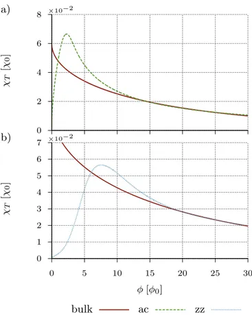
In Fig. 7 the flux dependence of the bulk result, Eq. (52), is compared with the numerically calcu- lated contribution from the conduction and valence band to χ of an (a) armchair and (b) zigzag tri- angular quantum dot at µ= 0. The thermal en- ergies of the bulk systems are chosen such that β(bulk)h∆ ¯E(bulk)iφ≈β(ac,zz)h∆ ¯E(ac,zz)iφ. By choosing lower thermal energies finite size effects gain importance and deviations from the bulk theory emerge as can be seen from Fig. 8: The susceptibilitiesχT of the quantum dots exhibit oscillatory behavior which becomes all the more pronounced, as the thermal energies tend to lower values. In this case all parameters are chosen as in Fig. 7 but the thermal energy of the quantum dots is one order of magnitude smaller, i.e. 1/β(ac,zz)≈10−3t. For these parameters, the function F(α, γ), Eq. (53), reaches posi- tive values only in the considered flux range. Therefore χT, Eq. (52), is diamagnetic. This holds also true for the numerically calculated contributionχT of the triangular quantum dots. From the definition (35) of α∝∆LL/µ one expects the bulk effects to dominate over finite-size signatures and therefore good agreement of the numeri- cal data with the bulk calculations forφ&15 φ0. This is confirmed by Figs. 7 and 8.
For lower values ofφEq. (51) is no longer valid yielding deviations from the tight-binding calculations as the os- cillatory modulations ofχT demonstrate in Fig. 8. These oscillations are smeared out due to the larger thermal en- ergies chosen in Fig. 7. In both figuresχT of the quan- tum dots reaches zero for ϕ ≈ 0 and χT is morevoer suppressed on a finite flux interval, φ.3φ0 in Fig. 8a) and φ. 7φ0 in b), respectively. This behavior can be understood in view of the energy spectra of the quantum dots, Fig. 2. In each case there is a small gap between E= 0 and the first non-zero energy level as a signature of confinement. For thermal energies smaller than this gap andµ= 0 there are no occupied states above the Dirac point besides the edge states of the zigzag quantum dot contributingϕ-linear to ΩT and yieldingχT = 0. In the case of the armchair quantum dot ΩT and therefore χT
vanish completely in this specific parameter range.
3. Regime: γ <1and arbitraryα
If the thermal energy of the system is larger than the level spacing, also states above the Fermi level are oc- cupied implying that tuning the chemical potential or the magnetic field does not lead to a discontinuity of the corresponding contribution to the grand potential. As a consequence the susceptibility is expected to be a smooth
0 2 4 6
a) 8 ×10⁻²
χT[χ0]
0 1 2 3 4 5 6 7
0 5 10 15 20 25 30
φ[φ0]
b) ×10−2
χT[χ0]
bulk ac zz
FIG. 7: Flux dependence of the temperature dependent susceptibility contribution χT of bulk graphene compared with the numerically calculated contribution of triangular nanostructures with a) armchair and zigzag b) edges of side length L ≈100a. The chemical potential is chosen at µ = 0 and the thermal energies are 1/β(ac,zz)≈10−2t and 1/β(bulk)≈1.5·10−1tin panel a) and 1/β(bulk)≈1.7·10−1t in panel b), such that Eq. (18) holds true. The scaling fac- tors γ(ac)≈2.5·10−2 and γ(zz)≈3.8·10−2 are obtained by
fitting.
function of these parameters. In this parameter range the magnetic flux and the thermal energy can be chosen in such a way that the Landau level clustering in the quan- tum dot spectra is pronounced enough to make the bulk theory valid, on the one hand, and effectively wash out the finite size signatures on the other hand. Hence one can expect good agreement of the bulk theory with the susceptibility of the quantum dots.
Using again the decomposition of the Fresnel integral into smooth and oscillatory part, one can start from rep- resentation Eq. (38) of the field-dependent part of Ω.
0 0.5 1 1.5
a) 2 ×10⁻²
χT[χ0]
0 0.5 1 1.5
0 5 10 15 20 25 30
φ[φ0]
b) ×10−2
χT[χ0]
bulk ac zz
FIG. 8: Same as Fig. 7 for smaller thermal energies 1/β(ac,zz)≈10−3t and 1/β(bulk)≈1.44·10−1t in panel a) and 1/β(bulk)≈1.42·10−1t in panel b), such that Eq. (18) holds true. The scaling factors γ(ac)≈3.9·10−3 and
γ(zz)≈7.8·10−3 are obtained by fitting.
SubstitutingE= 2/β x+µgives Ω =˜ K
2√ 2πϕ3/2
∞
X
m=1
√1 m3
Im
Z∞
0
du 1
√u(u−i)
× Z∞
−∞
dxsech2(x) e−uπm(2xγ+1α)2eiπm(2xγ+α1)2
. (54)
Forγ <1 the complex phase rapidly oscillates as a func- tion ofxfor all values ofα. Therefore the second integral can be solved within stationary phase approximation:
Z∞
−∞
dxsech2(x) eiπm(2xγ+α1)2≈ |γ|
2√
msech2 γ 2α
eiπ4.
(55) UsingR∞
0 du[√
u(u−i)]−1=πexp (−iπ/4) in (54) yields Ω˜ ≈ K
4√ 2
√ϕ3|γ|sech2 γ 2α
X∞
m=1
1
m2 (56)
=g
A(~vF)2π2
12βsech2 γ 2α
ϕ2, (57)
whereP∞
m=1m−2=π2/6 is used. The corresponding ex- pression for the total orbital susceptibility reads
χ(µ) =−µ0g
φ20 (~vF)2π2 6 βsech2
µ β 2
(58)
=χ0(B)×
√2π2
9ζ 32γsech2 γ 2α
. (59)
−4.3632
−4.3630
−4.3628
−4.3626
−4.3624
−4.3622
−4.3620
−4.3618
a) ×10−1
χT[χ0]
−9.5709
−9.5706
−9.5703
−9.5700
−9.5697
−9.5694
−9.5691
−9.5688
0 0.1 0.2 0.3 0.4 0.5
µ[t]
b) ×10−1
χT[χ0]
bulk ac zz
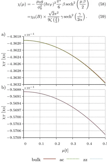
FIG. 9: Comparison of the temperature-dependent suscepti- bility contribution χT for bulk graphene with that of a tri- angular armchair a) and zigzag b) graphene flake as a func- tion of the chemical potential at a magnetic flux ofφ= 5φ0
and 1/β(ac,zz) = 5t. The corresponding values used in the analytic expression for the bulk are 1/β(bulk) ≈ 2.1t in a) and 1/β(bulk) ≈ 2.9t in b). The fitted scaling factors are
γ(ac)= 0.44, γ(zz)= 1.7.
In this regime the divergent contribution χ0 of the filled valence band is compensated by the contribution χT of the thermally excited charge carriers leading to a distinctly diamagnetic and moreover flux independent magnetic response. This result can also be found in the literature2–5. The contribution χT =χ−χ0 can be ex- tracted from Eq. (59) reading
χT(µ) =−χ0(B)
"
1−
√2π2
9ζ 32γsech2 γ 2α
#
. (60) Since√
2π2/[9ζ(3/2)]≈0.6 and sech2(x)≤1,∀x∈Rthe contribution χT exhibits paramagnetic behavior in this
parameter range. The comparison of this bulk contri- bution with numerical data for the triangular armchair and zigzag quantum dot in Fig. 9 a) and b) shows perfect agreement as expected at larger fluxes.
To fulifil γ < 1, i.e. p
A/(2π)ϕ < kBT /(~vF), in the limit of very low temperatures requires that |En|, Eq. (12), tend to zero even for large Landau indices n.
Hence a change in the magnetization of bulk graphene due to weakly thermally excited charge carriers can only occur for Fermi energies close to the Dirac point. For T→0 this leads to a sharply peaked susceptibility at µ = 0. In view of Eq. (32), this can be deduced from Eq. (58) yielding the well known expression2,4–11
χ(µ)−β−−−→∞→ −µ0g
φ20 (~vF)22π2
3 δ(µ). (61) This limit is not truly reachable numerically for the finite systems considered since the Landau level structure is not pronounced enough as it can be seen from Fig. 2.
Another limit of physical relevance concerns µ→0 or α→ ∞. In this limit the total orbital susceptibility reads
χ(µ)−−−→ −µ→0 µ0g
φ20 (~vF)2π2
6 β∝ − 1
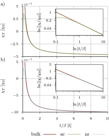
kBT. (62) This typical temperature dependence, already known in the literature3, is also affirmed by the numerical data, see Fig. 10. The double logarithmic graphs in the insets show clearly the 1/kBT dependence in the limit µ→ 0 (for φ = 5φ0). The difference between the bulk the- ory and the numerical data for small thermal energies reflects, on the one hand, the limit of validity of the an- alytical approximation forγ < 1; on the other hand, it is a signature of finite-size effects which gain importance in the low temperature limit.
IV. OSCILLATORY FINITE-SIZE EFFECTS FOR GRAPHENE NANOSTRUCTURES
A. General semiclassical framework
Semiclassical periodic orbit theories offer a distin- guished way to analytically describe finite-size effects en- coded in the energy spectra of spatially confined systems of arbitrary shape. Boundary effects are incorporated in the semiclassical approximation of the oscillatory part of the DOS, ρoscsc (E). One important criteria for applying such semiclassical approximations, the Gutzwiller trace formula47 for chaotic classical dynamics or the Berry- Tabor trace formula48 for regular classical dynamics, re- quires that the linear system size lies in a mesoscopic regime, kL 1, where k= E/(~vF) is the Fermi wave number. In general,doscsc (E) is of the form
doscsc (E) =X
γ
doscsc,γ(E), (63) doscsc,γ(E)∝ReDγe~iSγ, (64)
−5
−2.5 0 2.5
a) 5 ×10⁻¹
χT[χ0]
−10
−5 0 5
0 2 4 6 8 10
1/β[t]
b) ×10−1
χT[χ0]
0.04 0.2 1
0.1 1 10
ln [t/β]
ln[|χ/χ0|]
0.04 0.2 1 5
0.1 1 10
ln [t/β]
ln[|χ/χ0|]
bulk ac zz
FIG. 10: Comparison of the numerical data of the orbital magnetic susceptibility contributionχT of a triangular arm- chair a) and zigzag b) graphene flake atφ = 5φ0 with the analytic result for bulk graphene in the limitµ→0. In both cases the correspondence is convincing fort/β >1 as for lower thermal energies this approximation loses validity. The scal- ing factors attainγ(ac)≈5.8 andγ(zz)≈8.6 which is in agree- ment with the condition|E¯(bulk)−E¯(ac)|<|E¯(bulk)−E¯(zz)|.
The insets show both the full orbital magnetic susceptibilityχ in a double logarithmic plot and confirm the scaling behavior
χ∝ −β at the Dirac point.
where the sum runs over infinitely many classical peri- odic orbits γ with classical action Sγ =H
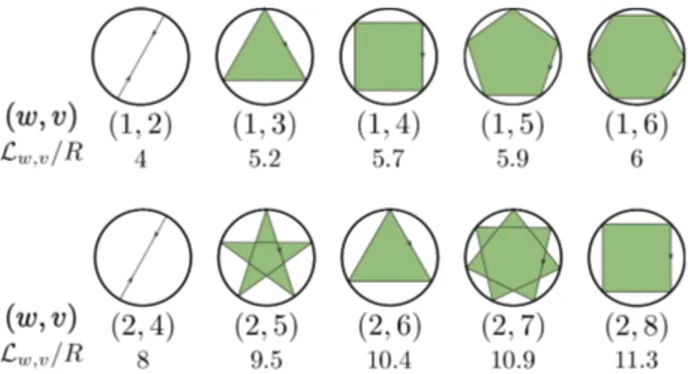
γdq·p=pLγ and length Lγ. The exact form of the classical ampli- tudeDγ sensitively depends on the specific geometry of the system and can be calculated either within the recipe given by Gutzwiller47 in the case of non-integrable clas- sical dynamics or within the recipe of Berry and Tabor48 when the classical dynamics is integrable. In the latter case, relevant in the following, the summation overγ in Eq. (63) runs over families of degenerate orbits, as de- picted in Fig. 11a) for a disk geometry. This degeneracy of orbits in a regular billiard can be described in terms of continuous symmetry groups G such that the mem- bers of a specific orbit family are related to each other through the action of a group element g of G. This is already included in the Berry-Tabor trace formula48 for field-free regular systems. In the case of small symmetry breaking, as it is caused by an weak external magnetic
field, one has to take these degeneracies separately into account as discussed in Subsec. IV B. Therefore, we will associate an orbit familyγ with the corresponding ele- mentgof the underlying symmetry groupGif necessary, i.e. γ7→γ(g).
In Refs. [20, 21, and 49] the authors show in a gen- eral way, how the trace formulas for ¨Schr¨odinger bil- liards¨ with classically regular or chaotic dynamics can be extended to an arbitrary shaped, field-free graphene flake including the most common types of boundaries, i.e. zigzag, armchair and infinite-mass-type edges. Re- sembling Eq. (63) the semiclassical trance fromulas for graphene read
ρoscsc (E) =X
γ
ρoscsc,γ(E), ρoscsc,γ(E)∝doscsc,γ(E)TrKγ, (65) where doscsc,γ is given by Eq. (63), of the corresponding Schr¨odinger system. Hence, thedoscsc,γ contain all informa- tion about the orbital dynamics in the graphene system.
The additional factor TrKγ denotes a trace over the pseu- dospin propagator Kγ of the orbit γ and contains only graphene specific information about the boundary. In Refs. [49, 21] a general expression for TrKγ of an orbit, withNγ reflections at the boundaries is derived, yielding
TrKγ = 4fγcos θγ+π
2Nγ cos
2KΛγ+ϑγ+π 2Nγ
, (66) if the total number of reflections on armchair edges,Nac, is even and TrKγ = 0 otherwise. The prefactor is defined as fγ = i3Nγ−Nzz, where Nzz denotes the number of re- flections on zigzag edges.θγ =PNγ
i=1θiis the sum over all reflection angles along the orbitγ. K= 4π/(3a) denotes the distances between the Dirac points and the Γ point of the Brillouin zone. Λγ =PNac/2
i=1 (x2i−1−x2i) is the sum over the distance between two subsequent reflections on armchair edges. Furtherϑγ=PNzz
i=1(−1)siϑidenotes the sum over zz reflection anglesϑi, where ϑi=±θi for re- flection on A- and B-edges, respectively, and si is the number of ac reflections occuring after the zz reflection i. One finds21,49 TrKγ = TrKγ−1 whereγ−1 denotes the time reversed partner of orbitγ,
B. Semiclassical approximation of the orbital magnetic susceptibility
In Ref. [16] the authors showed how the semiclassic theory of integrable and non-integrable billiard systems with parabolic dispersion can be extended to include the effect of an homogeneous, constant magnetic field.
Due to the formal similarity of the trace formulas of sys- tems with parabolic dispersion, Eq. (63), and graphene, Eq. (65), the techniques used in Ref. [16] can be readily transferred. We will focus on the low-field regime where the classical cyclotron radius Rc =k l2B is much larger