Nonperturbative comparison of clover and highly improved staggered quarks in lattice QCD and the properties of the ϕ meson
Bipasha Chakraborty,1,2,* C. T. H. Davies,1,† G. C. Donald,3 J. Koponen,1,4 and G. P. Lepage5
(HPQCD Collaboration)‡
1SUPA, School of Physics and Astronomy, University of Glasgow, Glasgow G12 8QQ, United Kingdom
2Jefferson Lab, 12000 Jefferson Avenue, Newport News, Virginia 23606, USA
3Institute for Theoretical Physics, University of Regensburg, 93040 Regensburg, Germany
4INFN, Sezione di Tor Vergata, Via della Ricerca Scientifica 1, I-00133 Roma, Italy
5Laboratory of Elementary-Particle Physics, Cornell University, Ithaca, New York 14853, USA (Received 3 April 2017; published 2 October 2017)
We compare correlators for pseudoscalar and vector mesons made from valence strange quarks using the clover quark and highly improved staggered quark (HISQ) formalisms in full lattice QCD. We use fully nonperturbative methods to normalize vector and axial vector current operators made from HISQ quarks, clover quarks and from combining HISQ and clover fields. This allows us to test expectations for the renormalization factors based on perturbative QCD, with implications for the error budget of lattice QCD calculations of the matrix elements of clover-staggered b-light weak currents, as well as further HISQ calculations of the hadronic vacuum polarization. We also compare the approach to the (same) continuum limit in clover and HISQ formalisms for the mass and decay constant of theϕmeson. Our final results for these parameters, using single-meson correlators and allowing an uncertainty for the neglect of quark-line disconnected diagrams are:Mϕ¼1.023ð6ÞGeV andfϕ¼0.238ð3ÞGeV in good agreement with experi- ment. The results come from calculations in the HISQ formalism using gluon fields that include the effect ofu, d,sandcquarks in the sea with three lattice spacing values andmu=dvalues going down to the physical point.
DOI:10.1103/PhysRevD.96.074502
I. INTRODUCTION
Weak decay matrix elements calculated in lattice QCD are critical to the flavor physics programme of overdeter- mining the Cabibbo-Kobayashi-Maskawa matrix to find signs of new physics (see, for example, [1,2]). For this programme it is particularly important to study heavy flavor physics and, although it is now becoming possible to study heavy quarks using relativistic formalisms [3,4], the most extensive studies of heavy quarks in lattice QCD have been done with nonrelativistic formalisms (or at least formalisms that make use of nonrelativistic methods), such as NRQCD[5]or the Fermilab formalism [6]. In nonrelativistic formalisms a critical issue is the normalization of the current operator that couples to the W boson, and this is one of the main sources of error in the lattice QCD result. Relativistic formalisms can be chosen to have absolutely normalized currents, for example through the existence of a partially conserved axial current (PCAC) relation [7]. The main issue with relativistic formalisms is then controlling discretization errors [8].
The archetypal heavy meson weak decay process is annihilation of aB meson toτν. The hadronic parameter which controls the rate of this process is theBmeson decay constant,fB, proportional to the matrix element to create a Bmeson from the vacuum with the temporal axial current containing a bottom quark field and a light antiquark field.
When the heavy quark field uses a nonrelativistic formal- ism the simplest way to match the appropriate current in lattice QCD to that in a continuum scheme is using lattice QCD perturbation theory. Such calculations of theZfactors required have been done throughOðαsÞfor both NRQCD [9–11]and Fermilab[12,13]heavy quarks with a variety of different light quark formalisms. The most recent results for Bmeson decay constants using NRQCD are given in[14]
and using Fermilab heavy quarks in[15].
In doing these calculations for Fermilab heavy quarks and clover light quarks[12]it was noticed that the heavy- light current renormalization differed very little atOðαsÞ from the square root of the product of Z factors for the temporal vector heavy-heavy and light-light currents, which can be determined nonperturbatively. This then gives rise to the possibility of determining, for example, ZA4
hl with small uncertainty if it can be demonstrated that this result is true to all orders in perturbation theory and is not specific to only one light quark formalism (or heavy
*bipasha@jlab.org
†christine.davies@glasgow.ac.uk
‡http://www.physics.gla.ac.uk/HPQCD
quark formalism). This question is a critical one for the reliability of the estimates of perturbative errors in deter- minations of fB andfBs and other weak matrix elements using this approach. The same issues arise, for example, for the vector current with implications for the matrix elements calculated for B→πlν from lattice QCD[16].
Here we test this fully nonperturbatively for the case where the“heavy-light”current is made of a clover quark (≡Fermilab formalism at low mass) and a highly improved staggered quark (HISQ) [8] both tuned accurately to the strange quark mass, following the suggestion in[1]. We use the absolute normalization for the HISQ-HISQ temporal axial vector current that arises from chiral symmetry in that formalism to normalize both the HISQ-clover and clover- clover temporal axial vector current. By determining the normalization of the appropriate vector currents, also fully nonperturbatively, we can then determine the ratio used by the Fermilab collaboration and test it against the hypothesis that it should be close to 1.
From the samesquark propagators for the study above we can also make vector (ϕ) meson correlators and study theϕ meson mass and decay constant for the cases where theϕis made purely of clover quarks or purely of HISQ quarks, or made of one of each. Our results cover three values of the lattice spacing spanning the range from 0.15 fm to 0.09 fm and so we can compare the approach to the continuum limit of the two formalisms (and test whether they have a common continuum limit) for the two calculations.
Finally we make a more extensive analysis of theϕmeson using the HISQ formalism covering a more complete range of gluon field ensembles that includes multiple values of the u=dquark mass in the sea going down to the physical value, and allowing physical results to be derived. Our calculation uses single-meson correlators only and neglects quark-line disconnected diagrams (which we expect to have negligible impact). Our results tend to confirm that the impact of coupling theϕto itsKK¯ decay mode is small and increases theu=dquark mass-dependence of the ϕproperties deter- mined in lattice QCD. We are able to obtain theϕmass and decay constant to an accuracy of a few MeVand in agreement with experiment. Understanding the properties of theϕfrom lattice QCD is important because it provides a good vector final state for alternative studies of semileptonic weak decay rates compared to the usual pseudoscalar final states. For example, Vcs can be determined from Ds→ϕlν given lattice QCD results and experimental rates [17–19]. Bs→ ϕlþl− is potentially an important rare decay mode for searches for new physics[20].
The paper is laid out as follows: SectionIIdescribes the background to our calculation; the perturbative studies of the renormalization factors that have been done for current operators using different actions and combinations of actions, and the general picture that emerges that needs to be tested nonperturbatively. Section III describes our lattice calculation to do these tests and gives our results for
the nonperturbative determination of Z factors for the HISQ-clover and clover-clover case, showing how the nonperturbative determination backs up the picture seen perturbatively. We also compare discretization effects in the clover and HISQ formalisms through the properties of theϕ meson using the Z factors we have obtained to normalize the decay constant. SectionIVgives our results for the mass and decay constant of theϕin the HISQ formalism only, coveringu=dquark masses down to the physical value and allowing a chiral/continuum extrapolation to the physical point. SectionVgives our conclusions. Appendix Acon- siders the renormalization factors for currents with NRQCD heavy quarks and Appendix B uses our results for the renormalization factors for local vector currents for HISQ quarks to extrapolate to values on finer lattices.
II. BACKGROUND
To provide accurate physical results for hadronic matrix elements, lattice QCD current operators must be renormal- ized to match to those in continuum QCD. For some currents and quark formalisms absolute normalization is possible; for example for the temporal axial current in formalisms with sufficient chiral symmetry. In other cases a renormalization Zfactor must be determined as accurately as possible. Since the Z factor, beyond tree level, allows for the difference between gluon radiation in the continuum and that in the presence of the lattice momentum cutoff, it is an ultraviolet quantity and can be determined in QCD perturbation theory.
Lattice QCD perturbation theory is relatively complicated and such calculations have generally been restricted to the determination of effects atOðαsÞonly.Zis then determined by equating the one-loop scattering amplitude between on shell quark states in continuum QCD and on the lattice.
Early calculations in which a heavy quark in the Fermilab formalism[6]was combined with a clover light quark found that the heavy-light current renormalization [12]differed very little atOðαsÞfrom the square root of the product ofZ factors for the temporal vector heavy-heavy and light-light currents. This was found also to be true for Fermilab heavy quarks and asqtad light quarks [13].
Specifically, the Fermilab Lattice collaboration writes for the temporal axial vector current:
ZA4
hl ¼ρ ffiffiffiffiffiffiffiffiffiffiffiffiffiffiffiffiffiffiffi ZV4
hhZV4 ll
q ð1Þ
where
ρ¼1þρð1Þαsþρð2Þα2sþ ð2Þ andρð1Þis found to be very small (typically<4π×0.01) if the heavy quark mass is not too large. Note then that this is a relationship valid for“light”heavy quarks and not in the infinite quark mass (static) limit. In practice the region of small values ofρð1Þextends for heavy quark masses,mh, in
the Fermilab formalism up to thebquark mass at least for fine lattices, witha <0.1fm. For small values ofmh the Fermilab formalism becomes identical to the standard tadpole-improved clover formalism.
ZV4
hh andZV4
ll are the renormalization factors for local temporal vector currents made respectively of Fermilab formalism quarks and light quarks in whatever formalism is being used for the heavy-light current. These vector current Z factors can be determined fully nonperturbatively in lattice QCD by demanding normalization of the vector form factor between two identical mesons at rest.
Equation(1)then gives rise to the possibility that ZA4 hl
can be determined with small errors if it can be shown thatρ is indeed close to 1 to all orders in perturbation theory. The argument that this should be true is based on the idea that a large part of the perturbativeZcomes from the self-energy of the individual quark legs and this part will cancel in ρ [12]. This cancellation will include tree-level mass depend- ence and tadpole effects. However, this only guarantees that ρð2Þand higher coefficients should be“of reasonable size,” not that they should be as small asρð1Þis found to be. The question of what uncertainty it is reasonable to take for the missingα2sand higher order pieces is then a critical one for the reliability of the estimates of perturbative errors in determinations of fB and fBs and other weak matrix elements using this approach.
In testing this relationship nonperturbatively we note that to be robust it must be fairly general and work for a variety of formalisms, for example any light quark formalism com- bined with a Fermilab formalism heavy quark. Since in fact it is a relationship that works best for light quarks in the Fermilab formalism, we can substitute standard clover quarks for Fermilab quarks since the Fermilab formalism becomes the clover formalism in the light quark mass limit.
This avoids then any need to handleΛ=mh(wheremhis the heavy quark mass) corrections to the“heavy-light”currents.
We then test Eq.(1)for the case where the current on the left-hand side contains two light quarks that use different formalisms. One formalism is clover, representing the Fermilab formalism. For the other formalism we could use the asqtad staggered formalism to test directly the results from[13]. However it makes more sense to use the current state-of-the-art staggered formalism, HISQ[8], since we will also use the state-of-the-art MILC collaboration gluon field configurations that include u,d,sandcquarks in the sea using the HISQ formalism. We will tune the masses of the valence light quarks to that of the strange quark because this can be done very accurately[21,22]using the pseudoscalar
“strange-onium”meson, theηsand will give higher statistical accuracy for this test than using lighter quarks.
Because the HISQ formalism has a remnant chiral symmetry it has an absolutely normalized temporal axial current. By comparing the matrix element between the vacuum and the ηs of temporal axial currents made of clover quarks or mixed currents with one clover and one
HISQ quark to that made of HISQ quarks we can determine the Z factor for the clover-clover current and the HISQ- clover current. We can also readily determine theZfactors for the local temporal vector current made of HISQ quarks or of clover quarks, or the mixed HISQ-clover current, by setting the vector form factor to 1 between twoηsmesons made of appropriate quark formalisms at rest.
We then have all the Z factors necessary to test the relationship equivalent to Eq.(1):
ZJH−cl ¼ρJ
ffiffiffiffiffiffiffiffiffiffiffiffiffiffiffiffiffiffiffiffiffiffiffiffiffi ZV4
cl−clZV4 H−H
q
; ð3Þ
where H stands for HISQ and cl for clover, for the cases where the current J is the temporal axial current or the temporal vector current. In both cases we can determine how close to 1 ρJ is and therefore how small the perturbative coefficients that make upρJ must be.
As a side product of these calculations we can test a number of other relationships betweenZfactors, including that between the temporal axial vector and temporal vector currents in all three combinations of formalisms, H-H, H-cl and cl-cl. Note that the Z factor being determined on the left-hand side of Eq.(1)is a flavor-nonsinglet current.
Our equivalent expression, implied by Eq. (3), then also corresponds to a flavor-nonsinglet current even though both quarks ares quarks. This means that we do not need to consider any quark-line disconnected contributions to the correlation functions that we are using for this analysis. The ZV factors on the right-hand side of Eq.(1)correspond to vector currents for quarks of the same flavor; in this case quark-line disconnected contributions are negligible [23]
and can be ignored.
The next section describes the lattice calculation and gives results for theseZ factors.
III. Z FACTORS
A. Lattice configurations and simulation parameters We use gluon field ensembles generated by the MILC collaboration[24]at widely differing values of the lattice spacings: 0.15 fm, 0.12 fm and 0.09 fm. The relative lattice spacings were fixed using a determination ofw0=a [22].1 wherew0is the Wilson flow parameter[25]. The absolute value of w0 was determined from fπ [22] to be 0.1715 (9) fm. The gluon field ensembles include the effect ofu,d, sandcquarks in the sea (with degenerateuanddquarks) using the HISQ formalism and also use a gluon action improved fully throughOðαsa2Þ[26]. We therefore expect the gluon fields to have very small“intrinsic”discretization errors which is useful for studying the discretization errors of meson correlation functions made on these configura- tions using different quark formalisms.
1Note that the value on set 8 has changed from that given in[22];
we are grateful to C. McNeile for providing this updated value.
For our determination of cloverZfactors we have chosen to use the ensembles 1, 3 and 8 that have a sea light quark mass in units of the sea strange massml=ms¼0.2. This is for reasons of numerical speed since these lattices have relatively modest size of 3.5 fm. Since we are calculating meson correlation functions made purely of strange quarks, we expect sea quark mass effects to be small so the fact that mseal is not physical is not an issue. Finite volume effects were shown to be negligible for theηs for lattices of size 3.5 fm in [27] (see also Sec. IV). In any case we would expect such effects to be the same for the HISQ and clover valence quarks and hence any effects should cancel in the ratios we use to determineZ factors.
On gluon field ensembles 1, 3 and 8 we calculate valence HISQ and clover quark propagators using the standard HISQ action [8] (as used for the sea quarks) and the standard tadpole-improved space-and-time-symmetric clo- ver action used for light quarks[28]. In the clover action the gluon fieldsUμare divided by a tadpole parameter[29],u0, for which we use the fourth root of the plaquette. The parameter values are listed in TableII.
For the source for each propagator we divide the spatial slice of the lattice at a given time value into23cubes and use a Gaussian random number for each color at the spatial points corresponding to the corners of each cube. We use many time sources on each configuration to improve statistics (see TableII) and they are evenly spaced through the lattice. The starting time source for each configuration is chosen randomly to reduce autocorrelations, which are small for ηs correlators [30].
We combine the HISQ propagator with its complex conjugate into a pseudoscalar meson correlator (two-point function) that corresponds to the ‘Goldstone taste’ in the parlance of staggered quarks. In spin-taste notation this is γ5⊗γ5 and the correlator simply corresponds to the modulus squared of the propagator, summed over a spatial slice of the lattice to project onto zero spatial momentum.
We will denote the ground-state particle of this correlator ηH−Hs . To obtain the ground-state parameters we fit the correlator to the standard multi-exponential form as a function of time separationtbetween the source and sink:
C2pt ¼nXexp−1
k¼0
a2kfðEk; tÞ;
fðEk; tÞ ¼e−Ektþe−EkðLt−tÞ: ð4Þ There are no staggered quark“oscillating”terms in the ηs
correlator because it is of Goldstone taste and made of equal mass quarks. Our fits use Bayesian methods[31]that allow us to include multiple exponentials and consequently allow for systematic errors in our ground-state parameters from contamination from excited states. We use a prior width on all of the amplitudes of 0.5 (larger than any of our ground-state amplitudes) and on the ground-state energy of 0.05 (much larger than any of our fit uncertainties on this
parameter). On the energy differences between consecutive states we take a prior of 0.8(0.4) GeV (converted back to lattice units in the fit). We have checked that the ground- state parameters from our fit are very insensitive to the priors. We drop the very smalltvalues from the fit, taking tminof 3 or 4. Fit results and uncertainties are stable from 3 or 4 exponentials upwards withχ2=dof varying from 0.5 to 0.9. We take our final values from the 6 exponential fit.
Neither the number of exponentials in the fit, nor thetmin value have any significant effect on the result for ground- state parameters. We illustrate this in Fig. 1, giving the ground-state energy from the fit as a function of the number of exponentials included for both tmin of 3 (the value we used) andtmin¼10. Fortminof 3 fits with a small number of exponentials (1 and 2) give a poor fit because higher states contribute to the correlator at small t values.
However, once the fit does have a good χ2 it remains stable as further states are added to the fit. Fortminof 10 a good fit can be obtained with fewer states included and it agrees with the result usingtmin¼3. We prefer to take the smallertminvalue for uniformity of fits across all the 2- and 3-point functions we study here.
Here we are concerned with the properties of the ground state, which are given byk¼0. These are the mass of the ηH−Hs which is given in lattice units by E0 and its decay constant which is determined from the ground-state ampli- tude,a0, as described in Sec.III B.
Earlier results [22] using a variety of both u=d and s HISQ valence masses on the more complete set of ensembles from TableIallowed us to determine the value of the ηs mass in the continuum and chiral limits of full lattice QCD. Although the ηs meson is not a physical particle (because we do not allow it to mix with other flavorless pseudoscalars) it is nevertheless useful in lattice QCD for tuning thesquark mass[21]. In[22]we obtained a physical value for theηs mass of 688.5(2.2) MeV. Here we then tune the bare quark mass in our HISQ action to obtain this value for theηH−Hs mass [combining our results FIG. 1. Results for the ground-state energy,E0in lattice units, for the H-Hηs on coarse set 3 as a function of the number of exponentials used in the fit [Eq.(4)]. We show results for atmin value of 3 and 10; the results are shown with dashed lines for fits where theχ2=½dof>1.
forE0 from Eq. (4)with the values of the lattice spacing from Table I] on each ensemble. The bare valence quark masses obtained are given in TableII. Note that these values are not the same as those used in[22] because, with the benefit of those results, we have improved the tuning (see also[32]). Theηsmass values in lattice units (E0from our fits) are given in Table III. The precision of the values shows how well this tuning can be done.
We also combine clover quark propagators with their complex conjugates to makeηscorrelators using either the temporal axial current,ψγ¯ 4γ5ψ, or the pseudoscalar current,
¯
ψγ5ψ, at both source and sink. We then fit these correlators simultaneously to the same fit form, Eq.(4), given earlier for the H-H case and using the same priors. We require both correlators to have the same energies but different ampli- tudes,ak;A4andak;P. Again the ground-state parameters are given byk¼0and are the ones we use here. The ground- stateηcl−cls mass is given by combining values forE0with the inverse lattice spacing obtained from Table I. The mass parameter in the clover action is denoted byκwith the bare quark mass being related to1=ð2κÞby an additive constant [28]. We tuneκto give the sameηsmass as that discussed for the H-H case above. Table II gives the tuned κ values we obtain and TableIIIgives theηs masses in lattice units (E0from our fits). Again we are able to perform this tuning very precisely.
The third option is to combine a clover and HISQ propagator to make a mixed-action correlator. To do this the HISQ propagators, which have no spin component, must be converted back to naive quark propagators with a spin component by “undoing” the staggering transformation used to obtain the staggered quark action[8,33]. Because we have used a“corner wall”source for our propagators, with one point per23block, the matrices implementing the staggered transformation at the source are all the unit matrix, which simplifies the combination. Once converted to a naive form with four spin components the HISQ TABLE I. Sets of MILC configurations used here with their
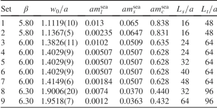
(HISQ) sea quark masses, ml (mu¼md¼ml), ms and mc in lattice units. β¼10=g2 is the QCD gauge coupling andw0=a [22,32]gives the lattice spacing,a, in terms of the Wilson flow parameter,w0[25]. The lattice spacing is approximately 0.15 fm for sets 1 and 2; 0.12 fm for sets 3–7 and 0.09 fm for sets 8 and 9.
The lattice size is L3s×Lt. Ensemble sizes are 500 to 1000 configurations each.
Set β w0=a amseal amseas amseac Ls=a Lt=a 1 5.80 1.1119(10) 0.013 0.065 0.838 16 48 2 5.80 1.1367(5) 0.00235 0.0647 0.831 16 48 3 6.00 1.3826(11) 0.0102 0.0509 0.635 24 64 4 6.00 1.4029(9) 0.00507 0.0507 0.628 24 64 5 6.00 1.4029(9) 0.00507 0.0507 0.628 32 64 6 6.00 1.4029(9) 0.00507 0.0507 0.628 40 64 7 6.00 1.4149(6) 0.00184 0.0507 0.628 48 64 8 6.30 1.9006(20) 0.0074 0.0370 0.440 32 96 9 6.30 1.9518(7) 0.0012 0.0363 0.432 64 96
TABLE II. List of parameters used for the valence quarks.
Column 2 gives the HISQ bare mass. Columns 3 and 4 give the cloverκvalue and the tadpole factoru0used to tadpole-improve the action. Column 5 gives the number of configurations used for most of the calculations and column 6 the number of time sources on each configuration. Because our HISQ valence quarks are much faster to calculate we have determinedηs H-H correlators on double the number of configurations for sets 3 and 8. We only determined the three-point correlators for the H-cl current on half of the configurations on set 8, however. The final column gives the T values used in the determination of 3-point correlation functions.
Set amsH;val κscl;val u0 ncfg nt 3pt T
1 0.0705 0.14082 0.85535 1021 12 9, 12, 15, 18 3 0.0541 0.13990 0.86372 527 16 12, 15, 18, 21 8 0.0376 0.13862 0.87417 504 16 16, 19, 22, 25
TABLE III. Results from the fits toηsmeson correlators made from HISQ-HISQ, clover-clover and HISQ-clovers quark propagators. Column 3 gives the ground-state mass in lattice units. The H-H and cl-cl results are very close as a consequence of tuning the bare mass parameters in the HISQ and clover actions. Column 4 gives theηs decay constant in lattice units for the H-H case where it is absolutely normalized. Column 5 gives the unnormalizedηs
decay constant for the cl-cl and H-cl cases. Column 6 gives theZfactors for the cl-cl and H-cl cases from setting the decay constant equal to that in the H-H case.
Set Action comb’n aMηs afηs afηs=ZA4 ZA4
1 H-H 0.54024(15) 0.14259(8)
cl-cl 0.53966(30) 0.19682(26) 0.7245(10)
H-cl 0.57330(24) 0.16303(24) 0.8746(13)
3 H-H 0.43135(9) 0.11399(4)
cl-cl 0.43141(20) 0.15242(18) 0.7478(9)
H-cl 0.44698(17) 0.12946(16) 0.8804(11)
8 H-H 0.31389(7) 0.08287(4)
cl-cl 0.31328(12) 0.10664(16) 0.7771(12)
H-cl 0.31821(11) 0.09338(13) 0.8874(12)
propagators can be straightforwardly combined with clover propagators as in the clover-clover case above and using a temporal axial current operator at source and sink, or a pseudoscalar operator. To fit these correlators (simultane- ously) we must include oscillating terms that arise from the staggered quark formalism. The fit form is then
C2ptðtÞ ¼Xnexp
k¼0
a2kfðEk; tÞ−ð−1Þt=aXnexp
ko¼0
a2kofðEko; tÞ; ð5Þ with normal (nonoscillating) amplitude parametersak, and amplitudes for oscillating terms given byako. Again we use priors for the normal terms that are the same as those given above for both the H-H and cl-cl cases. For the oscillating terms we use the same amplitude and energy difference priors as for the normal terms and we take the difference between the energy for the ground state in the oscillating channel and that in the normal channel to be 0.6(4) GeV. We again take the fit results from the 6 exponential fit, given stability of the results from the 3 or 4 exponential fit upwards. Since the mass parameters have now all been tuned, the mass we obtain for the ground-state particle in this H-cl channel gives us information about discretization effects. These masses are given in Table III and we can see that they become increasingly close to the masses for the H-H and cl-cl channels as the lattice spacing becomes smaller moving from set 1 to set 8. This will be discussed further in Sec.III F.
B. Z factors for A4
The decay constant of theηsmeson can be defined as the matrix element between the meson and the vacuum of the temporal axial current. When the meson is at rest this is given by
h0jA4jηsi ¼Mηsfηs: ð6Þ For the HISQ action, remnant chiral symmetry gives a partially conserved axial current (PCAC) relation connect- ing the temporal axial and pseudoscalar currents for the Goldstone taste pseudoscalar that we use here. Thus we can determine an absolutely normalized decay constant from the relation
fηs ¼2msa0 ffiffiffiffiffiffi
2 E30 s
; ð7Þ
whereE0anda0are the ground-state energy and amplitude respectively from the fit given in Eq.(4). Results for the decay constant in lattice units are given in TableIII. These agree with those from[22]at the physicalsquark mass (see Fig.3 in that reference).
For the clover action we do not have a PCAC relation and so the temporal axial current must be renormalized. We do this by equating the decay constant obtained from the ground-state amplitude in the cl-cl case to that obtained in the H-H case where we have an absolute normalization. In
the cl-cl case we can convert the ground-state amplitude from our fits obtained from meson correlation functions using the temporal axial current to an unnormalized decay constant value in lattice units using
afηs=ZA4 ¼a0;A4
ffiffiffiffiffiffi 2 E0 s
: ð8Þ
The results of this determination are given for each ensemble in Table III. The renormalization factor ZA4 is then obtained by settingafηs in the cl-cl case equal to that obtained in the H-H case.
An alternative method, but one that we do not use, would be to set the cl-cl decay constant equal to the physical value of 181.14(55) MeV obtained in [22]. Because the discre- tization effects seen in the H-H values offηs are so small this would make little difference—at most 0.5% on set 1.
Exactly the same arguments and procedure apply to determiningafηs=ZA4andZA4in the H-cl case. In this case, because theηs mass is not exactly the same as the tuned value there is a difference between matching decay con- stants and matching matrix elements (fηsMηs). Because the difference in mass is a discretization effect we have chosen to match decay constants. The differences between doing this and matching the matrix elementfηsMηsare as large as 6% on set 1, but fall to 1% on fine set 8, and act in the direction of makingZA4 smaller than that quoted. We can use this variation to assess the size of nonperturbative effects appearing in our nonperturbative determination of theZfactors. A 6% effect on the coarsest lattices is not a surprising result;ðaΛÞ2withΛaround a few hundred MeV would give something similar.
The values ofZA4 for the cl-cl and H-cl current are then given in column 5 of TableIII.
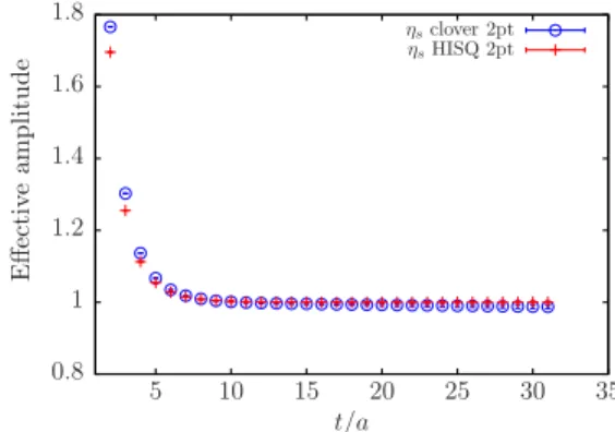
Figure2illustrates directly how similar the H-H and cl-cl correlators in terms of theirt-dependence. The figure shows the result in each case of dividing the correlator (with the
FIG. 2. The effective amplitude defined as the correlator divided by the fit result for the ground-state exponential for H-H Goldstone and cl-cl pseudoscalarηscorrelators on coarse set 3. The number of configurations used for the H-H correlators is double that of the cl-cl correlators.
pseudoscalar current at source and sink) by the fit function a20fðE0; tÞ corresponding to the ground state. The central value of both effective amplitudes is then 1 at large times. The statistical uncertainties in the H-H case are about 2.5 times smaller than the cl-cl case when double the number of configurations was used. The results for the two amplitudes agree well away from the central plateau region, showing that the contributions of excited states to the correlators are also well matched. Discretization errors give differences at small times.
Another interesting feature of Fig.2is that the statistical error in the correlator increases with time, albeit slowly. In the simplest picture of how noise arises in meson corre- lators this would not happen because the signal to noise ratio should be a constant for pseudoscalar meson corre- lators made of quarks with equal mass. The variance of the meson correlator is a correlator made of two quarks and two antiquarks. When the quark masses are the same the ground-state energy of this combination is twice that of the meson that controls the signal, in the absence of interactions between the two mesons and ignoring a
“crossed” diagram that would need to be calculated to determine fully the two-meson correlator. It is these latter two effects that complicate the simple picture and cause the mass controlling the noise to fall below that controlling the signal so that an exponentially growing (albeit slowly) signal-to-noise ratio results. See [34–36] for earlier dis- cussion and analysis of correlator noise.
C. Z factors for V4
The normalization of temporal vector currents in lattice QCD is readily obtained by demanding that the vector form factor be 1 between two identical states at rest. Here we can implement this forηs states so that
ZV4hηsjV4jηsi ¼2Mηs: ð9Þ The matrix element of the vector current is calculated from a 3-point function as illustrated in Fig.3. Propagator 2 is generated from propagator 1 as a source and then joined at the temporal vector vertex to propagator 3. Appropriate spin combinations are taken at the two ends to ensure that source and sink correspond to pseudoscalar mesons. Sums over spatial slices ensure that source and sink mesons are at rest. We use four values for the value ofTat the end-point of the three-point function. This enables us to fit both the t-dependence (for0≤t≤T) and theT-dependence of the three-point function to reduce systematic errors from excited state contamination. The values used for T are listed in Table II.
By choosing combinations of HISQ and clover propa- gators we can determine the renormalization factor for H-H, cl-cl and H-cl temporal vector currents. The temporal vector currents we consider are all local operators and for the H-H case this corresponds to the spin-taste structure
γ4⊗γ4. Because this current is not a taste singlet we cannot use a three-point function made purely of staggered quarks but must have a nonstaggered “spectator” quark (propagator 1 in Fig.3). Here it is natural to use a clovers quark, extending our earlier method that used NRQCD quarks [37], itself based on a Fermilab Lattice/MILC method that uses clover quarks[15].
First we discuss the case of the cl-cl temporal vector current. For this case, all propagators are cloversquarks and we use the pseudoscalar operator at the source and sink to make ηs mesons. We make this choice because the pseudoscalar operator gives somewhat more precise corre- lators; the two-point functions are simply the squared modulus of the propagator in that case. We then fit the three-point functions from allTvalues simultaneously with two-point cl-cl (usingγ5at source and sink)ηscorrelators.
The fit form for the three-point function is given by:
C3pt ¼X
i;j
aiVijajfðEi; tÞfðEj; T−tÞ ð10Þ
where ai and aj are amplitudes from the two-point functions [Eq. (4)]. We use a prior width on the Vij of 0.0(3.0) (along with priors on all other parameters as for the earlier two-point correlator fits). Using a relativistic nor- malization of states the matrix element of the lattice temporal vector current between ground-state ηs mesons at rest is given by2E0V00 and therefore
ZV4 ¼ 1
V00: ð11Þ Our results for each of sets 1, 3 and 8 are listed in TableIV. Notice that the numbers are a lot more precise than those forZA4. Figure4plots the ratio of the three-point correlator for each value ofTto that of the two-point correlator atT, as a function of t to illustrate the quality of our results.
From Eq.(10)this ratio will be1=V00for all values oft, up to contamination from excited states. It is clear from Fig.4 that this contamination is under good control, with FIG. 3. A diagram to show how our three-point correlation functions are constructed. All of the quark propagators, denoted 1, 2 and 3 are forsquarks and combined at times 0 andTto make ηs mesons. A temporal vector current is inserted at t.
all three-point functions showing a good plateau at the same value. Note, that we do not use this ratio in our fits, but instead perform a full multi-exponential fit to our correlators as given in Eqs.(10) and(4).
For the H-H local temporal vector current we have a H-cl ηs correlator at source and sink (made with aγ5operator).
This means that there are additional oscillating terms in the fit form for the three-point function in a simultaneous fit with the appropriate two-point correlators. The fit function is then
C3pt ¼X
i;j
aiVijbjfðEi; tÞfðEj; T−tÞ
−ð−1ÞðT−tÞ=aX
i;jo
aiVijobjofðEi; tÞfðEjo; T−tÞ;
−ð−1Þt=aX
io;j
aioViojbjfðEio; tÞfðEj; T−tÞ;
þX
io;jo
aioViojobjofðEio; tÞfðEjo; T−tÞ: ð12Þ
Againai,bj,aioandbjoare amplitudes that appear in the two-point correlator fit [Eq.(5)]. We take a prior width onVij of 0.0(3.0) and on the other V of 0.0(1.0). Again the renormalization factor for the local temporal vector current is given by Eq.(11)and our values are given in TableIV. These results improve on the values used by us[27,38]in the calculation of the hadronic vacuum polarization contribution to the anomalous magnetic moment of the muon.
Lastly the H-cl temporal vector current is obtained from three-point functions in which propagator 3 is a HISQ quark and 1 and 2 are clover quarks, using theγ5operator to construct mesons. Again we fit the three-point correlators simultaneously with the appropriate two-point correlators.
Here we need both H-cl and cl-cl two-point correlators. Our three-point function fit form has oscillatory terms on the side corresponding to the H-cl two-point function but none on the side corresponding to the cl-cl two-point function, so the fit form is the first two lines of Eq.(12). We use the same priors as above and again the renormalization factor for the local temporal vector current is given by Eq.(11).
Note that in using this equation we are ignoring small discretization effects between the H-clηsmass and the cl-cl ηs mass evident in TableIII. Including this effect changes theZV value by less than 0.05% even on the very coarse lattices. Our results are given in TableIV.
We see in Table IV that the values for ZV4 are very similar to those forZA4 in the H-cl and cl-cl cases, despite being rather far from 1. This does add weight to the idea that there is a component of theZfactor that comes from the“clover wave function renormalization” and could be canceled in ratios.
D. Results for ρA4 and ρV4
We now have all the ingredients necessary to test the formula for the off-diagonal-in-action renormalization fac- tor in terms of the square root of the product of diagonal temporal vector renormalization factors given in Eq. (3) [testing Eq.(1)]. We can do this for both temporal axial vector TABLE IV. Column 4 gives results for the renormalization factor for the local temporal vector current for each of
the different action combinations and each ensemble listed in columns 1 and 2. Results forZV4in the H-H case are more precise than those given in[27]becaue those were taken from preliminary fits. Column 3 repeats results from TableIIIfor the temporal axial vector. Columns 5 and 6 then give theρfactors defined in Eq.(3)for the off-diagonal H-cl combination for both temporal axial vector and temporal vector currents. Errors are statistical/fitting errors combined from the different components in quadrature.
Set Action comb’n ZA4 ZV4 ρA4 ρV4
1 H-H 0.9881(10)
cl-cl 0.7245(11) 0.7262(2)
H-cl 0.8746(13) 0.8660(7) 1.0325(16) 1.0223(9)
3 H-H 0.9922(4)
cl-cl 0.7478(9) 0.7397(3)
H-cl 0.8804(11) 0.8739(7) 1.0277(12) 1.0201(8)
8 H-H 0.9940(5)
cl-cl 0.7771(12) 0.7620(3)
H-cl 0.8874(12) 0.8839(8) 1.0196(14) 1.0156(10)
FIG. 4. The ratios of the average three-point correlator to average two-point correlator showing how the same plateau value is reached for four different values of T: 16,19,22 and 25 using the clover action on fine set 8. Statistical errors are shown on the points.
and temporal vector currents using the data in TableIV, and the results for theρfactors are also given in that table. The ρfactors are indeed close to 1 in all cases, demonstrating that the perturbative series forρdoes have small coefficients for all powers ofαs. Note that the temporal vector and temporal axial vectorρfactors are even closer to each other than they are to 1. In Fig.5we plot our values forρA4andρV4against the square of the lattice spacing.
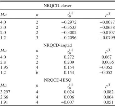
In Fig.5we also compare to theOðαsÞperturbative result for the operator made from a combination of clover and asqtad staggered quarks in the limit that both quark masses go to zero[13]. In the clover-asqtad case theOðαsÞcoefficient forρfor bothA4andV4isþ4π×3.04×10−3¼0.0382,2 the same because of the chiral symmetry of the asqtad action.
In Fig. 5 we combine this coefficient with a value of αs
determined in the V-scheme at scale2=awhich corresponds approximately to the BLM scale found for these operators in the clover-clover case [12]. The appropriate values of αs
on sets 1, 3 and 8 are: 0.356, 0.314 and 0.269. From these values it is clear that missing α2s terms in the perturbative expansion could be sizeable; a coefficient of 1 would give a 10% shift toρ.
Since we are using the HISQ action for the staggered quark and not the asqtad action, the perturbative results quoted above are not correct for our case, and are provided purely for a qualitative comparison. However we see that the nonperturbative H-cl and the one-loop perturbative asqtad- cl results have similar values and behave in a similar way with lattice spacing. The nonperturbative results are slightly further from 1 on the coarser lattices. On the finer lattices they agree to within 1%, with the perturbative result being 1% from 1 and the nonperturbative result 2%. Any com- parison of nonperturbative and perturbative results must take
account of possible systematic discretization effects in the nonperturbative results. As discussed in Sec.III Bwe can estimate these from the impact of changing our definition of ZA4. This produces a sizeable 6% effect on the coarsest lattices but falling to 1% on the finest lattices. Thus on the finest lattices we can give an error band of1%around our 2% difference from 1 for theZ factor and expect the full perturbative result to lie in this band. If the one-loop perturbative results fall in this band, as the asqtad-cl results do, we can conclude that higher order terms in the perturba- tive expansion are constrained at this 1% level.
Assuming that the H-cl one-loop perturbative coeffients are similar to those for asqtad-cl,3which seems likely, we can conclude that our nonperturbative results confirm the scenario in which a one-loop perturbative QCD determi- nation ofρJ is a very good approximation. The uncertainty from missing higher orders in the mixed action renormal- ization factor can then be assumed to be small on the basis of the known (one-loop) coefficients.
The Fermilab-MILC asqtad-clover heavy-light calcula- tions are carried out at very different values for the clover quark mass than that of thesquark that we have used here.
They find, however, that the one-loop value for ρ varies relatively slowly with mass, becoming even closer to 1 as the clover mass increases to that of the charm quark[13].
Their most recent paper onBmeson decay constants[15]
with Fermilab heavy quarks and asqtad light quarks uses gluon field configurations with similar lattice spacing values to those used here. They take the uncertainty from missing higher order terms in the perturbative expansion of ρas 0.1α2s with αs taken as αVð2=aÞ on the fine lattices.
This gives a 0.7% uncertainty from missing higher orders in the perturbative matching of the heavy-light current.
Although at first sight this uncertainty looks very small for anOðαsÞcalculation we can see from our results that it is in fact reasonable, provided that the H-cl one-loop calculation gives a very similar result to the asqtad-cl one-loop coef- ficient. This uncertainty is compatible with the difference we see between our nonperturbative results and the one-loop perturbation theory (for asqtad-cl), allowing for discretiza- tion effects in the nonperturbative results.
In Appendix A we show how this approach to the determination of renormalization constants also works when the heavy quark uses the NRQCD formalism. For an NRQCD-light current the division by the square root of the Z factor for the vector light-light current removes sizeable effects in the one-loop coefficients associated with the light quark formalism for clover and asqtad light quarks; no such effect is present, or correction needed, for the NRQCD quark. Defining the heavy-lightZ factor using Eq.(1)then reduces the one-loop coefficient in the perturbative piece of theZfactor from around 0.3 to around FIG. 5. Our nonperturbative results for theρfactors defined in
Eq. (3) and given in Table IV for current operators made by combining HISQ and clover quarks. Green open circles gives results for the temporal axial vector currentA4and green pluses the results for the temporal vector currentV4. Also shown are the one-loop perturbative lattice QCD results for mixed asqtad-clover currents with light clover quarks (orange bursts).
2Note a typographical error in[13]has introduced a minus sign.
3Preliminary indications, for which we thank E. Gámiz, are that this is the case.
0.05, with an associated reduction in perturbative uncer- tainty, given the evidence shown here. For NRQCD-HISQ currents the method is no longer useful since neither NRQCD nor HISQ has significant“wave function renorm- alization” effects and the one-loop coefficients in Z are around 0.05 without the use of Eq.(1).
We can also ask: to what extent can our results for ρ, shown in Fig.5, be used to constrain unknown higher order terms in the perturbative expansion forρ? To test this we fit a functional form to ρ that includes a power series inαs
allowing for discretization effects. We use ρða;αsÞ ¼Xni
i¼0
ciþdi
aΛ π
2 þfi
aΛ π
4
αis ð13Þ
with c0¼1.0, Λ¼0.5GeV and αs taken in the ‘V’ scheme at scale2=a. Priors onci, di andfi are all taken as 0(1). Good fits (withχ2=½dofof 0.3) are readily obtained to the results for both ρA4 andρV4 with ni¼5 (although changing ni has very little effect). The fit result for c1 is 0.0(1), compatible with being small, as found in the calculation for the asqtad-cl case [13]. The other ci are not constrained by the data, however. If instead we givec1a prior of 0.04(4) to make it close to that for the asqtad-cl case, thenc2is weakly constrained by the fit to be around zero with an uncertainty of 0.3. These features are again compatible with the perturbative series for ρhaving small coefficients. Given an αs coefficient for the H-cl case, an improved constraint on the α2s coefficient would be pos- sible. We show how this works in AppendixBwhere, given an OðαsÞ coefficient, we are able to extrapolate the ZV results for the H-H case to finer lattices fairly accurately.
E. Further tests of renormalization factors In staggered formalisms there are multiple versions of bilinear operators corresponding to different “tastes.” In determining the pseudoscalar ss¯ meson decay constant in Sec.III Bwe used the local pseudoscalar operator (in spin- taste notationγ5⊗γ5) because this operator is connected to the partially conserved temporal axial current through the PCAC relation. Note that we do not actually form operators with the partially conserved temporal axial current because it is point split and so quite complicated to implement.
It is also unnecessary since we can use the simple local pseudoscalar operator. On some occasions, however, it is necessary or desirable to use an explicit temporal axial current operator. The simplest one is the local operator, in spin-taste notationγ4γ5⊗γ4γ5. This couples to the “local non-Goldstone” ηs meson which has a slightly heavier mass than the Goldstone meson whose mass was used to tune the squark mass in Sec.III A.
Here we give results forηsmeson correlators that use this local temporal axial current operator at source and sink.
The fits to these two-point correlators have staggered
“oscillations” and we use the fit form given in Eq. (5).
In fact we fit these correlators simultaneously with the Goldstoneηscorrelators, although the fits have no param- eters in common. The ground-state mass,E0, corresponds to the mass of theηsmeson of this taste and differs from the Goldstone ηs mass by discretization effects. This will be discussed further in Sec.III F. The ground-state amplitude, a0, can be converted into an unrenormalized decay constant using the formula of Eq.(8). As in Sec.III Bwe can define a renormalization constant from setting this decay constant equal to that obtained from the Goldstone ηs where the normalization is absolute.
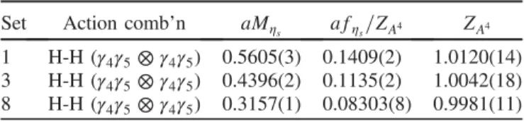
TableVgives our results on sets 1, 3 and 8 for the mass, decay constant andZA4 factor for the H-H local temporal axial current case. We see thatZA4is very close to 1 on all sets. The chiral symmetry of the HISQ action also means thatZA4 for the local temporal axial vector current should equal that for the local temporal vector current[39]up to lattice artefacts and we demonstrate that this is true below.
Note that we would get slightly different values forZA4if we matched the matrix element (fηsmηs) between the tastes rather than just the decay constant. This is because the meson masses differ for different tastes by an amount proportional to αsa2. Since this is a pure discretization effect, we do not include it. Doing so would give values for ZA4that are 4% lower on set 1 and 0.6% lower on set 8, and in fact then closer toZV4 on the coarser lattices.
The comparison of temporal axial vector and temporal vectorZfactors can now be done for all the combinations of actions we have used—H-H, H-cl and cl-cl. The HISQ action has sufficient chiral symmetry that the H-cl and H-H Zfactors should be the same up to lattice artefacts from the nonperturbative determination that vanish asa→0, and we can test this. For H-H the appropriateZfactors are those for the local temporal vector (γ4⊗γ4) from Table Vand the local temporal axial vector (γ4γ5⊗γ4γ5) from TableV. For the other cases both results come from TableIV. Figure6 shows the ratio ofZA4=ZV4 as a function of lattice spacing.
We see that, although the ratio differs from 1 by 2% for H-H and 1% for H-cl on the very coarse lattices, the discrepancy between theZfactors for H-H and H-cl is falling witha2to agree to better than 1% on the fine lattices. Results are consistent with theZfactors being in complete agreement in the continuum limit in keeping with our expectation based on chiral symmetry.
TABLE V. Results from the fits toηs meson correlators made from HISQsquarks with the local temporal axial current operator (in spin-taste notationγ4γ5⊗γ4γ5). Column 3 gives theηsmass for this taste of meson and columns 4 and 5 the unrenormalized decay constant and derived renormalization for this current as discussed in the text.
Set Action comb’n aMηs afηs=ZA4 ZA4
1 H-H (γ4γ5⊗γ4γ5) 0.5605(3) 0.1409(2) 1.0120(14) 3 H-H (γ4γ5⊗γ4γ5) 0.4396(2) 0.1135(2) 1.0042(18) 8 H-H (γ4γ5⊗γ4γ5) 0.3157(1) 0.08303(8) 0.9981(11)
For the cl-cl case, in the absence of chiral symmetry, we do not expectZA4 andZV4 to agree. In one-loop perturba- tion theory the OðαsÞcoefficient for the ratio ZA4=ZV4 is þ0.127[40]for the Symanzik improved gluon fields and unimproved currents (along withcsw¼1to leading order inαs) that we use here (this is somewhat smaller than the coefficient of 0.163 for the unimproved gluon field case [41,42]). Thus we expectZA4=ZV4to be greater than 1. This is borne out by our results in Fig. 6. Our ratio is slightly below 1 on the very coarse lattices and moves above 1 going towards finer lattices, heading in the opposite direction to the other two action combinations. This is consistent with results heading towards the one-loop perturbative result, with the discrepancy on the coarser lattices being mainly a result of discretization effects. We have seen in Sec. III B that discretization effects can be Oð5%Þ on the coarsest lattices used here; they would presumably be smaller had we used an OðaÞ improved current. Using the αs values from Sec. III D would give one-loop results for ZA4=ZV4 of 1.045, 1.040 and 1.034 from very coarse to fine lattices to be compared with the values in Fig.6. Two-loop perturbative results forZfactors are available in the clover case[43]using an unimproved gluon action. There including two-loop terms pushesZA4
and ZV4 further below 1 for csw¼1 but makes less difference to their ratio.
Ratios of renormalization constants for two clover quarks are used by the Fermilab Lattice/MILC collabora- tions in their renormalization of form factors involving a b→cweak transition (for example, B→Dlν [44]). In that case the two quarks are both heavy but of different mass and Eq. (1) is used with l¼c. The perturbative analysis [45] again shows very small OðαsÞ coefficients for the ratio ρ, leading to the assumption that unknown higher order terms are also small. In this case Heavy Quark Symmetry arguments can also be used in arguments about the size of coefficients and their mass dependence.
The results that we have here are for the equal mass case at small mass and so rather far from the b→c scenario.
However the results for the one-loop perturbative renorm- alization given above are within 1% of our nonperturbative results on the fine lattices (as can be seen in Fig. 6), indicating that higher order corrections are indeed small in this case as in the H-cl case of Sec.III D.
F. Comparison of HISQ and clover discretization effects Systematic errors from discretization appear differently in the HISQ and clover actions and we can test how much of an effect that is from our results. The first place in which discretization effects show up is in differences between the masses ofηsmesons obtained with two quark propagators with the quark mass tuned to that of thesquark. Figure7 plots two mass differences in MeV against the square of the lattice spacing. One set of points gives the mass difference between the H-clηsmass and that of the H-H Goldstoneηs, using results from TableIII. The second set gives the mass difference between two tastes of H-H ηs, the local non- Goldstone and the Goldstone, using results from TablesIII andV. In both cases it is clear that the mass difference is purely a lattice artefact that vanishes asa→0. We expect the H-H mass difference to vanish asαsa2(since tree-level a2errors are absent from the action) anda4. In fact for the finer two points a simple fit to the formgðaΛÞ4þhðaΛÞ6 works well withΛa few hundred MeV and g andhwith priors 01; to add in the coarser point requires the addition of higher orders ina2 and/or αs. The H-cl mass difference has αsa terms from the clover action and the results are precise enough to see this. A fit to the results includinggαsðaΛÞ þhðaΛÞ2þjðαsðaΛÞ2Þhas aχ2=½dof of 0.9. The H-cl mass difference is larger and has a larger slope than the H-H mass difference plotted in Fig. 7.
FIG. 6. The ratio of renormalization constants for local tem- poral axial and local temporal vector currents made of our three combinations of actions: H-H (red open squares), H-cl (green open circles) and cl-cl (blue bursts). Results are plotted as a function of the square of the lattice spacing and compared to 1, shown as the grey dashed line.
FIG. 7. The mass difference between the HISQ-HISQ local non-Goldstone meson and the Goldstone meson (open red squares) plotted against the square of the lattice spacing. Also shown is the mass difference between the HISQ-cloverηs mass and that of the HISQ-HISQ Goldstoneηswhen both HISQ and clover action are tuned to thesquark mass (green open circles).
Errors include statistical errors and lattice spacing uncertainties correlated between the points.
It should be noted that the mass difference between the Goldstone and other tastes of H-H pseudoscalar meson would be larger[8,24]than the value plotted here for the local non-Goldstone to Goldstone splitting.
Since we use theηsdecay constant to fixZA4we cannot use that quantity to probe discretization effects in the cl-cl or H-cl cases. That the discretization errors are very small for the H-H case for this quantity has already been demonstrated in [22].
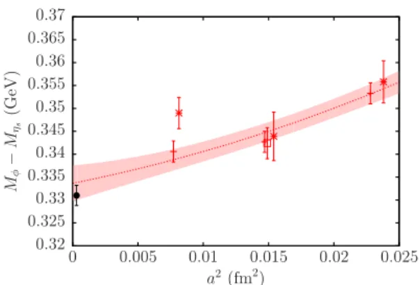
Two further quantities that we can study to compare discretization effects are the mass and decay constant of the vectorss¯ state, theϕ. To reduce the impact of uncertainties in the lattice spacing on our results we will in fact work with the mass difference between the ϕand theηs. Using the experimental value of theϕmass, 1.01946(2) GeV[46], this difference is 0.3310(22) GeV at zero lattice spacing and physical quark masses, where the uncertainty comes from the lattice determination of theηs mass[22].
The experimental value of the ϕ decay constant is determined from its partial width to leptons using (ignoring the spread in its mass from its full width):
Γðϕ→eþe−Þ ¼4π 3 α2QED
f2ϕ
Mϕe2s: ð14Þ Here αQED at the scale ofMϕis 1371 andes is thesquark electric charge in units of e (1=3). The experimental value of theϕ partial widthΓðϕ→eþe−Þ ¼1.27ð4ÞkeV [46], givingfϕ¼228.53.6MeV.
We construct vector meson correlators from s quark propagators in the same way as that described for ηs
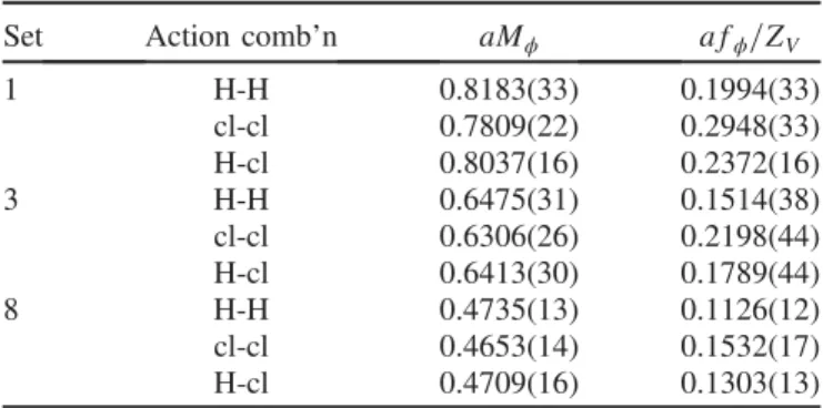
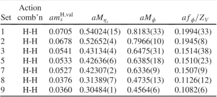
mesons, combining either two HISQ propagators, two clover propagators or a HISQ propagator and a clover propagator. The propagators are combined using the spatial version of the temporal vector current which was norma- lized in Sec. III C. We average over all three spatial directions for the current. The vector meson correlators (two-point functions) are fit as a function of time separation between source and sink using the methods and fit functions outlined in Sec. III A. We use the same priors as before; the only difference is that now the H-H correlators have an oscillating component and so we use the fit form of Eq.(5) rather than Eq.(4). TableVI gives results in lattice units for the ϕ mass and for its unnor- malized decay constant, afϕ=ZV, obtained from the ground-state amplitudes returned by the fit according to the vector analogue of Eq.(8)
afϕ=ZV¼a0;V ffiffiffiffiffiffi
2 E0 s
: ð15Þ
To normalize the decay constant we then multiply by the renormalization factor obtained for the temporal vector and given in Table IV, and by the inverse lattice spacing to convert to GeV units.
Results are plotted as a function of the square of the lattice spacing for each set of action combinations in Fig.8.
In order to test whether all the different combinations give the same continuum limit result, as they should, we have TABLE VI. The results for the mass and (unnormalized) decay constants of theϕmeson in lattice units from correlators made of s quark propagators generated using different combinations of HISQ and clover actions.
Set Action comb’n aMϕ afϕ=ZV
1 H-H 0.8183(33) 0.1994(33)
cl-cl 0.7809(22) 0.2948(33)
H-cl 0.8037(16) 0.2372(16)
3 H-H 0.6475(31) 0.1514(38)
cl-cl 0.6306(26) 0.2198(44)
H-cl 0.6413(30) 0.1789(44)
8 H-H 0.4735(13) 0.1126(12)
cl-cl 0.4653(14) 0.1532(17)
H-cl 0.4709(16) 0.1303(13)
FIG. 8. Top:mϕ−mηs calculated with different quark formal- isms and extrapolated toa¼0. Red bursts give results for mesons made with two HISQ quarks, blue pluses those made with two clover quarks and green open squares those made with one HISQ and one clover quark. The associated coloured bands give a simple continuum extrapolation fit with a common continuum limit, as described in the text. The black filled circle gives the value corresponding to the difference of the experimentalϕmeson mass the mass of theηsdetermined from lattice QCD[22]. It is offset slightly from a¼0 for visibility. Bottom: fϕ calculated for ϕ mesons made using quarks with different formalisms and extrapo- lated toa¼0. Symbols and coloured bands are as for the top plot.
The black filled circle is the value inferred from the experimental leptonic width of theϕ(see text).