Nonperturbative determination of improvement coefficients using coordinate space correlators in Nf

Nonperturbative determination of improvement coefficients using coordinate space correlators in N_f = 2þ1 lattice QCD

Piotr Korcyl^* and Gunnar S. Bali^†

Institut für Theoretische Physik, Universität Regensburg, D-93040 Regensburg, Germany (Received 9 August 2016; published 13 January 2017)

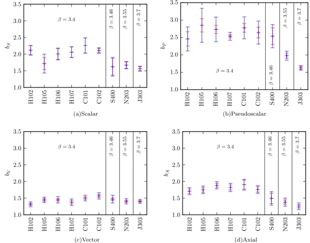
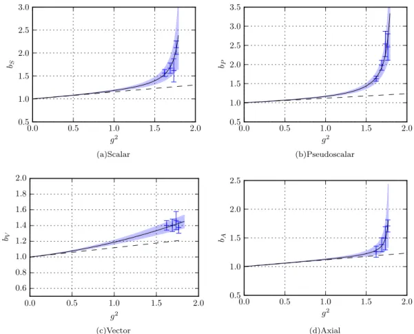
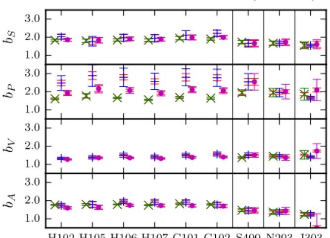
We determine quark mass dependent orderaimprovement terms of the formb_Jamfor nonsinglet scalar, pseudoscalar, vector and axialvector currents using correlators in coordinate space on a set of Coordinated Lattice Simulations ensembles. These have been generated employing nonperturbatively improved Wilson fermions and the tree-level Lüscher-Weisz gauge action atβ¼3.4, 3.46, 3.55 and 3.7, corresponding to lattice spacings ranging froma≈0.085fm down to 0.05 fm. In theN_f¼2þ1flavor theory two types of improvement coefficients exist:b_J, proportional to nonsinglet quark mass combinations, andb_J(orb~_J), proportional to the trace of the quark mass matrix. Combining our nonperturbative determinations with perturbative results, we quote Padé approximants parametrizing theb_Jimprovement coefficients within the above window of lattice spacings. We also give preliminary results forb~_J atβ¼3.4.

DOI:10.1103/PhysRevD.95.014505

I. INTRODUCTION

Lattice simulations of quantum chromodynamics (lattice QCD) have become an indispensable tool in particle and hadron physics phenomenology. By discretizing a quantum field theory on a lattice with a spacing a >0, ultraviolet divergences are regularized. At the same time this enables the numerical simulation of QCD, including its nonper- turbative dynamics. In principle such simulations need to be performed for different values of the lattice spacing, in order to remove the regulator by taking the continuum limit, a→0. In QCD this limit is approached as a polynomial ina, modulated by logarithmic corrections.

Obviously, many possible discretizations of the quark (and gluon) parts of the action exist. Staggered quarks suffer from conceptional problems, unless all fermions come in mass degenerate groups of four flavors. Also combining the flavor and spin degrees of freedom com- plicates operator mixing and the analysis of two- and three- point Green functions. Domain wall and overlap actions have the most desirable theoretical properties as even at a nonvanishing value of the lattice spacing these possess an (almost) exact chiral symmetry in the massless limit. In contrast, using Wilson fermions, chiral symmetry only becomes restored in the continuum limit, and also an additive mass renormalization is encountered. Wilson fermions, however, are computationally much less expen- sive to simulate and therefore offer the possibility of obtaining results at several values of the lattice spacing, enabling a controlled continuum limit extrapolation.

Unlike other fermion discretizations, where leading lattice artifacts are of ordera², for naive Wilson fermions

these are linear ina. Such terms can, however, be removed nonperturbatively[1,2], Symanzik improving[3]the action and the local operators of interest. Recently, within the Coordinated Lattice Simulations (CLS) effort [4], we embarked on a large scale simulation program, employing N_f ¼2þ1 flavors of order a improved Wilson- Sheikholeslami-Wohlert [5] (clover) fermions and the tree-level improved Lüscher-Weisz gauge action [6,7].

CLS use open boundary conditions in time [8], thereby increasing the mobility of topological charges and enabling us to maintain ergodicity at finer lattice spacings than had been possible previously. For details on the action, ensem- bles and parameter values, see Ref.[4].

As the cost of simulations increases with a large inverse power of the lattice spacing, we aim at not only order a improving the action but also all operators that will appear in matrix elements of interest. It is important to remove such contributions, that are linear in a, nonperturbatively since terms of order g^2νa, where g denotes the gauge coupling, will survive a (ν−1)-loop perturbative subtrac- tion. As g² varies only slowly with a, close to the continuum limit any g^2νa term will dominate over a² terms. The nonperturbative improvement of the action and of the massless axial current was carried out in Refs.[9,10]. In addition to such“c_J”improvement terms that persist in the massless limit, in the massive case additional b_J and b_J coefficients are encountered for a current J, for definitions, see, e.g., Ref. [11]. Existing results as of 2006 are reviewed in Ref. [12] and, more recently, for N_f¼2 clover quarks on Wilson glue, the combinations b_A−b_P and b_S¼−2b_m were determined nonperturbatively in Ref.[13].

Here we introduce a variant of the coordinate space method that was originally proposed in Ref.[14]. This will allow us to determine the scalar, pseudoscalar, vector

*piotr.korcyl@ur.de

†gunnar.bali@ur.de

and axialb_Jcoefficients, accompanying both flavor-singlet and nonsinglet quark mass combinations, with very limited computational effort. This is then successfully applied to the CLS ensembles described above.

This article is organized as follows. In Sec. II we describe the general approach and define the observables that will be studied. Next, in Sec. III we analyze these observables at tree level in lattice and continuum pertur- bation theory, including the leading nonperturbative effects, that are expected from the operator product expansion. This will allow us to improve the observables, to estimate the size of cutoff effects and to select the optimal set of separations at which the correlation func- tions are evaluated in the nonperturbative study. Then in Sec. IV we discuss systematic errors of our approach, addressing finite volume effects and estimating contribu- tions of nonperturbative condensates. Finally, in Sec. V we present results for all orderamcoefficients. In Sec.VI we conclude and present an outlook.

II. DESCRIPTION OF THE METHOD We generalize the method of Ref. [14]to the situation of N_f¼2þ1 nondegenerate quark mass flavors. For increased precision, we perturbatively subtract the leading order lattice artifacts. Furthermore, we employ the operator product expansion (OPE), enabling us to quantitatively describe medium distance corrections.

We will assume improved Wilson quarks and—as we aim at order aimprovement—we will consequently drop all terms of ordera². We remark that different prescriptions of obtaining improvement coefficients will in general give results that differ by such higher order corrections.

We denote quark mass averages following Refs.[11,15]

as

m_jk¼1

2ðm_jþm_kÞ; ð1Þ where

m_j¼ 1 2a

1 κj− 1

κcrit

: ð2Þ

The critical hopping parameter valueκcrit is defined as the point where the axial Ward identity (AWI) quark mass vanishes in the theory withN_f ¼3mass degenerate quark flavors.

We will label the mass of the two degenerate quark flavors asm₁¼m₂¼m_l and the mass of the remaining (strange) quark as m₃¼m_s. The mass dependence of physical observables can be parametrized in terms of the average quark mass

m¼1

3ðm_sþ2m_lÞ; ð3Þ

and the light quark massm₁₂ or, equivalently, the average of the strange and light quark masses m₁₃¹: if m and eitherm₁₂ orm₁₃ are known, m_l andm_s are fixed. Most ensembles have been generated following the strategy of the QCDSF Collaboration[16], keepingmconstant. This is supplemented by further ensembles at an (approximately) fixed value of the renormalized strange quark mass, as well as along the symmetric linem_l¼m_s [15].

A. General considerations and definitions We define connected Euclidean current-current correla- tion functions in a continuum renormalization schemeR, e.g.,R¼MS, at a scaleμ:

G^R_JðjkÞðx; m_l; m_s;μÞ ¼ hΩjTJ^ðjkÞðxÞJ^ðjkÞð0ÞjΩi^R: ð4Þ T denotes the time ordering operator, which we shall omit below as path integral expectation values are auto- matically time ordered. jΩi is the vacuum state and J∈fS; P; V_μ; A_μg. The current is defined as

J^ðjkÞ¼ψjΓJψk; J^ðjkÞ¼ψkΓ^†_Jψj; ð5Þ withΓJ∈f1;γ₅;γ_μ;γ_μγ₅g. ψj destroys a quark of flavor j∈f1;2;3gandxis a four-distance vector in coordinate space. As here we will only consider flavor nonsinglet currents, we always assumej≠k.

The above correlation function differs from that of the massless case by mass dependent terms[17–19],

G^R_JðjkÞðx; m_l; m_s;μÞ ¼G^R_JðjkÞðx;0;0;μÞ

×½1þOðm²x²; m²hFFix⁶; mhψψix⁴; mhψσFψix⁶Þ;

ð6Þ where at each order in m we only display the dominant type of term. Note that only even powers ofxcan appear above. Regarding the nonperturbative correction terms, the light quark condensate (in the MS scheme at the scale μ¼2GeV) reads hψψi ¼−Σ₀¼−½274ð3ÞMeV³ [20].

Recently, the renormalization group invariant nonperturba- tive gluon condensate hFFi was determined from a high order perturbative expansion in SUð3Þgauge theory[21], with the result hFFi∼ð530MeVÞ⁴ being larger than the original estimate hFFi∼ð330MeVÞ⁴ [22]. Unlike the quark condensate, this object is ill defined in principle and the uncertainty of its definition was determined to be similar in magnitude to its size [23,24]. The Wilson coefficient accompanying them²hFFiterm reads at leading order 1=12 for S and P and 1=6 for V and A [18,19], and hFFi=6∼ð340MeVÞ⁴, even if we assume the

1It is not necessary to differentiate between lattice and renormalized quark masses in the present context.

PIOTR KORCYL and GUNNAR S. BALI PHYSICAL REVIEW D 95,014505 (2017)

higher value[21]forhFFi. The mixed condensate[25]is usually estimated to be jhψσFψij∼0.8GeV²jhψψij∼ ð430MeVÞ⁵[26]. To leading order the Wilson coefficient accompanying this condensate readsm=2forSandP but vanishes for A and V [19]. We conclude that all mass dependent condensate contributions are bound by a respec- tive power of a scale Λ≈400MeV. Then, in the limit

x⁻²≫maxfm¹⁼³s Λ⁵⁼³; m¹⁼²_s Λ³⁼²; m²⁼³_s Λ⁴⁼³; m²_sg; ð7Þ the higher order terms in Eq. (6) can be neglected.

Assuming Λ> m_s≥m_l, we arrive at the condition x²≪1=Λ², i.e. jxj needs to be much smaller than 0.5 fm to permit neglecting mass dependent terms on the continuum side. In Sec.III below we will carry out a detailed analysis of the leading mass dependent corrections to Eq.(6).

The continuum Green functionG^Rabove can be related to the corresponding Green function G obtained in the lattice scheme at a lattice spacinga¼aðg²Þas follows:

G^R_JðjkÞðx; m_l; m_s;μÞ ¼ ðZ^R_JÞ²ð~g²; aμÞ

×ð1þ2b_Jam_jkþ6b_JamÞG_J^ðjkÞ;Iðn; am_jk; am;g²Þ;

ð8Þ

wherex¼na,n_μ∈Zso thatn²¼n_μn_μis integer valued and[1]g~²¼ ð1þb_gamÞg²is the orderaimproved value of the bare lattice couplingg²¼6=β. Not onlyZ^R_J but alsob_J andb_J will depend on g~² rather than ong², however, we can drop order a corrections to order a improvement coefficients and substitute b_Jð~g²Þ and b_Jð~g²Þ by b_Jðg²Þ andb_Jðg²Þ.

ExpandingZ^R_J aroundg² gives[15]

Z^R_J½~g²; aðg~²Þμ ¼Z^R_J½g²; aðg²ÞμÞ

1þ

∂lnZ^R_Jðg²; aμÞ

∂g² þ∂lnZ^R_Jðg²; aμÞ

∂lna

d lnaðg²Þ dg²

g²b_gamþ

¼Z^R_Jðg²; aðg²ÞμÞ

1þ

∂lnZ^R_Jðg²; aμÞ

∂g² − γJðg²Þ

4πβðg²Þb_gg²am

; ð9Þ

where

βðg²Þ ¼− 1 4π

dg²

d lna¼−g² 2π

β₀ g² 16π²þ

ð10Þ is the QCD β function in the normalization convention β₀¼11−²₃N_f. The anomalous dimension of the currentJ reads

γJðg²Þ ¼d lnZ_J

d lna ; ð11Þ

and is trivial for A_μ and V_μ. We can eliminate b_g by redefining

b~_Jðg²Þ ¼b_Jðg²Þ þb_gðg²Þ N_f

∂lnZ^R_Jðg²; aμÞ

∂g² − γJðg²Þ 4πβðg²Þ

g²: ð12Þ Both b_J and b~_J are of Oðg⁴Þ in perturbation theory. Z^R_J [27,28]andb_g ¼0.012000ð2ÞNfg²[1]are known toOðg²Þ and, therefore, the difference betweenb_Jandb~_Jis available to Oðg⁴Þ. However, the b_J coefficients are at present not available to this first nontrivial order. So the only thing we know is that b~_J ¼Oðg⁴Þ. Below we will also estimate these coefficients nonperturbatively. For practical purposes,

determiningb~_Jis sufficient as a knowledge ofb_Jis usually not required.

With the above redefinitions Eq. (8)reads

G^R_JðjkÞðx;m_l;m_s;μÞ¼½Z^RJðg²;aμÞ²×ð1þ2b_Jam_jkþ6~b_JamÞ

×G_J^ðjkÞ;Iðn;amjk;am;g²Þ: ð13Þ

The superscript I of J^ðjkÞ;I on the right-hand sides of Eqs.(8)and(13)refers to orderaimproved lattice currents:

S^ðjkÞ;I¼S^ðjkÞ,P^ðjkÞ;I¼P^ðjkÞ,V^ðjkÞ;I_μ ¼V^ðjkÞ_μ þiac_V∂_νT^ðjkÞ_μν , A^ðjkÞ;I_μ ¼A^ðjkÞ_μ þac_A∂_μP^ðjkÞ, whereT^ðjkÞ_μν ¼ψjσ_μνψk,σ_μν¼

i2½γ_μ;γ_νand∂_μdenotes the symmetric next neighbor lattice derivative:∂μfðxÞ ¼ ½fðxþaμÞˆ −fðx−aμÞ=ˆ 2a.

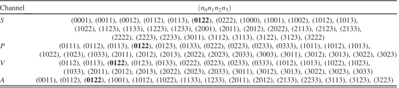
Here we will consider the following correlators:

G_SðjkÞðxÞ ¼ hS^ðjkÞðxÞS^ðjkÞð0Þi ¼G_SðjkÞ;IðxÞ; ð14Þ G_PðjkÞðxÞ ¼ hP^ðjkÞðxÞP^ðjkÞð0Þi ¼G_PðjkÞ;IðxÞ; ð15Þ

G_VðjkÞðxÞ ¼1 4

X

μ

hV^ðjkÞμ ðxÞV^ðjkÞμ ð0Þi

¼G_VðjkÞ;IðxÞ½1þOðaÞ; ð16Þ

G_AðjkÞðxÞ ¼1 4

X

μ

hA^ðjkÞμ ðxÞA^ðjkÞμ ð0Þi

¼G_AðjkÞ;IðxÞ½1þOðaÞ; ð17Þ

where we suppressed the argumentsm_jkandm. We remark that c_A is known nonperturbatively [10] for the action in use. In principle it can also be determined with coordinate space methods[14], tuningP

μh½A^I_μðx₁Þ−A^I_μðx₂ÞPð0Þi ¼0 for two Euclidean distances x₁≠x₂with x²₁¼x²₂. In this study we employ unimproved currents since mass inde- pendent orderacorrections cancel from the ratios that we will consider.

B. Description of the method

For the moment being we assumex²to be much smaller thanΛ⁻². Then the continuum Green function for massive quark currents is well approximated by the massless one and we can write

G^R_JðjkÞðx;0;0;μÞ^x2≪Λ≈⁻²½Z^R_Jðg²; aμÞ²

ð1þ2b_Jam_jkþ6~b_JamÞG_J^ðjkÞðn; amjk; am;g²Þ: ð18Þ Above we omitted mass independent order acorrections, which exist forJ¼VandJ¼A, see Eqs.(16)–(17), since these will cancel from the ratios that we are going to consider.

Obviously, in the massless limit, the ratio of two continuum Green functions G^R_JðjkÞðx;μÞ≡G^R_JðjkÞðx;0;0;μÞ for the same currentJ but different or the samejk flavor combinations cancels. We have discussed above that mass dependent corrections to this continuum ratio are propor- tional to orders ofx². Thus, we obtain

G_JðjkÞðn; am^ðρÞ_jk; am^ðρÞ;g²Þ G_JðrsÞðn; am^ðσÞrs; am^ðσÞ;g²Þ

¼1þ2b_Jaðm^ðσÞrs −m^ðρÞ_jkÞ þ6~b_Jaðm^ðσÞ−m^ðρÞÞ

þOða²; x²Þ; ð19Þ

where ρ and σ refer to different simulation points in the quark mass plane at a fixed value of the couplingg²and the indicesj; k; r; s∈f1;2;3grefer to the three flavors. While j≠kand r≠s,ρ¼σ is allowed. Combining results for different pairs of quark masses therefore enables us to determine the b_J and b~_J coefficients. Note that as only quark mass differences appear above, no knowledge ofκcrit

is required. This can only become relevant for the improve- ment of flavor singlet currents.

The leadingadependent correction terms can be of the types a²m², a²mΛ (for J¼V and J¼A), a³mΛ² and a³m=x²¼am=n². In contrast, the x²¼ ðnaÞ², x⁴ etc.

corrections are no lattice artifacts but have well-defined

continuum limits. This means that the determination of the improvement coefficients becomes possible forx²≪1=Λ² but the precision is limited by the size of1=n²¼a²=x², resulting in the windowa²< x²≪Λ⁻².

We remark that unlike in determinations of the renorm- alization constantsZ_J [29–31], as long asx²is within the above window, no knowledge on the functional form of G_JðxÞ is required to extract b_J and b~_J. Moreover, short- distance lattice artifacts are much reduced within the above ratio. Nevertheless, in Sec.IIIbelow we will correct for the leading order lattice artifacts as well as for the leadingx² andx⁴correction terms to Eq.(19), to broaden the window of distances where the method described can be applied.

C. Observable for thebJ coefficients

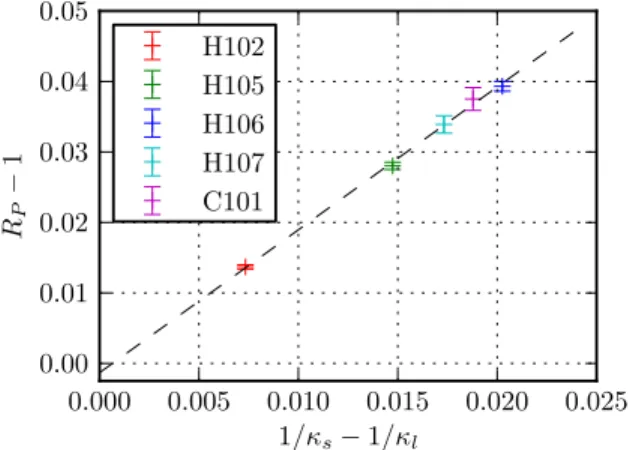
We consider a ratio R_Jðx; m₁₂; m₁₃Þ of two correlators evaluated on a single ensemble, i.e. we employ Eq.(19) with ρ¼σ. As m is fixed, R_J only depends on m_s−m_l¼2ðm₁₃−m₁₂Þ:

R_Jðx; ms−m_lÞ≡G_Jð12Þðn; am^ðρÞ₁₂; am^ðρÞ;g²Þ G_Jð13Þðn; am^ðρÞ₁₃; am^ðρÞ;g²Þ

¼1þ2b_Jaðm^ðρÞ₁₃ −m^ðρÞ₁₂Þ

¼1þb_J 1

κs− 1 κl

: ð20Þ

Hence,R_J−1is directly proportional tob_J, with a known prefactor that is independent of κcrit. Therefore, to deter- mineb_J, a single measurement at a simulation point with κ_l≠κs is sufficient.

In Fig. 1 we demonstrate this for J¼P, by showing R_Pðx; m_s−m_lÞ−1at a fixed separation x¼ ð0;1;1;1Þa and value of the lattice spacinga≈0.085fm (β¼3.4) as a function of 1=κs−1=κl. This is carried out on different

FIG. 1. Dependence of the ratioR_P−1at the separationx¼ ð0;1;1;1Þa as a function of the inverse hopping parameter difference1=κs−1=κl, see Eq.(20). For an ensemble list, see TableII.

PIOTR KORCYL and GUNNAR S. BALI PHYSICAL REVIEW D 95,014505 (2017)

ensembles. As expected, the data lie on a straight line whose slope is proportional tob_P. The intercept is at the origin as there are no mass independent orderaeffects in the current setting. The fact that a linear fit is consistent with this intercept demonstrates that the next-to-leading order lattice artifacts, that are proportional to m²a², are small at our quark mass values. The pointxshown in this example appears to be well suited for the extraction ofb_P. Below we will provide criteria to optimize this choice.

D. Observable for the b~J coefficients

In contrast to the improvement coefficients b_J accom- panying nonsinglet mass combinations, theb~_J coefficients can only be determined varying the average quark massm.

Again, we start from the ratio of correlation functions Eq.(19), where this time ρ≠σis necessary, i.e. informa- tion from at least two ensembles needs to be combined. The main set of CLS simulations [4] is obtained along a trajectory of constantm, where no sensitivity tob~_J exists.

However, we have points on two additional mass plane trajectories at our disposal (for details, see Ref.[15]), one along which only the light quark mass is varied while the AWI strange quark mass is kept constant and one line, along which κ_l¼κs¼κ^ðρÞ, i.e. m^ðρÞ ¼m^ðρÞ₁₂ ¼m^ðρÞ₁₃. A coefficient b~_J can most easily be obtained along this

“symmetric” trajectory, onceb_J is known, as in this case R~_Jðx; m^ðσÞ−m^ðρÞÞ≡G_Jð12Þðn; am^ðρÞ; am^ðρÞ;g²Þ

G_Jð12Þðn; am^ðσÞ; am^ðσÞ;g²Þ

¼1þ ð2b_Jþ6~b_JÞaðm^ðσÞ−m^ðρÞÞ

¼1þ ðb_Jþ3~b_JÞ 1

κ^ðσÞ− 1 κ^ðρÞ

: ð21Þ Note that again no knowledge ofκcrit is required. It is also possible to employ a pair of ensembles that differ in theirκs

value but share a similar κ_l value, eliminating the

dependence on b_J altogether when only light quark correlation functions are considered.

We demonstrate howb~_Pcan be extracted from the slope ofR~_Jin Fig.2: Using a set of threem_l ¼m_sensembles at β¼3.4, we evaluate the ratio of correlators for all three possible pairs of ensembles. Note that the statistical errors are much larger than in the case ofb_P, mostly because the numerator and denominator of Eq.(21)are uncorrelated.

III. BEHAVIOR AT SHORT AND LONG DISTANCES

In this section we discuss corrections to the ratios R_Jðx;ΔmÞ andRðx;~ ΔmÞ, see Eqs.(20)and(21), at large and short distances and define improved observables.

We employ Euclidean spacetime conventions throughout.

A. Continuum expectation

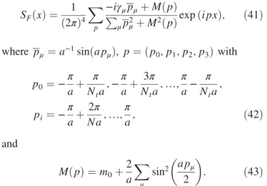
The components of the propagator S_FðxÞ≡S_Fðx;0Þ for a quark ψⁱα propagating from a four-position 0 to x are given as

S^ij_FαβðxÞ ¼ψⁱ_αðxÞψ^j_βð0Þ ¼−ψ^j_βð0Þψⁱ_αðxÞ; ð22Þ where α, β denote spinor and i, j color indices. This receives perturbative and nonperturbative contributions.

The massive free case propagator reads (see, e.g., Ref.[32])

S_FðxÞ ¼ 1 ð2πÞ²

γ_μx_μm²

x²K₂ðmjxjÞ þm²

jxjK₁ðmjxjÞ

¼ 1 2π²

γ_μx_μ x⁴

1−m²x² 4

þ m

4π² 1

x²þ…; ð23Þ whereK₁ðzÞ and K₂ðzÞare modified Bessel functions of the second kind. The leading nonperturbative contributions can be obtained, expanding

S^ij_FαβðxÞ ¼−ψ^j_βð0Þψⁱ_αð0Þ−x_μψ^j_βð0Þ½D_μψ_αⁱð0Þ þ : ð24Þ The color, spinor and Lorentz structure then implies that

hψ^j_βψⁱ_αi ¼bδ^ijδ_αβ; ð25Þ hψ^j_β½D_μψαⁱi ¼cδ^ijðγμÞ_αβ; ð26Þ where the constantsbandcare easily determined:

hψψi ¼X

i;α

hψⁱαψⁱαi ¼4Nb;

mhψψi ¼−γ_μhψD_μψi ð27Þ FIG. 2. Dependence of the ratio R~_P−1at the separation x¼

ð0;1;2;2Þa as a function of the inverse hopping parameter difference1=κ^ðσÞ−1=κ^ðρÞ.

¼−X

i;α;β;μ

ðγ_μÞ_αβhψⁱ_β½D_μψ_αⁱi

¼−cNX

μ

trγ_μγ_μ¼−16Nc: ð28Þ Above we made use of the equations of motion andN¼3 is the number of colors.

Collecting our results gives

S^ij_FðxÞ ¼fðxÞδ^ij1þg_μðxÞγ_μδ^ijþ ; ð29Þ fðxÞ ¼ m

4π² 1 x²− 1

4Nhψψi; ð30Þ g_μðxÞ ¼x_μ

1

2π²x⁴− m² 8π²x²þ m

16Nhψψi

: ð31Þ Note that some one-loop corrections to this expression can be found, e.g., in Ref. [33].

We are interested in correlation functions of the type

hJ^ð12ÞðxÞJ^ð12Þð0Þi ¼ h½ψ₁Γψ₂ðxÞ½ψ₂Γψ₁ð0Þi

¼∓htr½ΓS_F;2ðxÞΓγ5S_F;1ðxÞγ5i; ð32Þ whereS_F;j is the propagator of a quark of flavorjand we used theγ5-HermiticityS^†_Fð0; xÞ ¼γ5S_Fðx;0Þγ5. The upper signs refer toJ∈fS; P; Vgand the lower signs toJ¼A.² Note that as we restrict ourselves to nonsinglet currents, the Wick contraction yields only one term.

It is now easy to see that

hJ^ð12ÞðxÞJ^ð12Þð0Þi ¼∓N½f₁ðxÞf₂ðxÞtrðΓ²γ²₅Þ þg_1μðxÞg_2νðxÞtrðΓγ_νΓγ₅γ_μγ₅Þ

¼N½−4f₁ðxÞf₂ðxÞ

g_1μðxÞg_2νðxÞtrðΓγ_νΓγ_μÞ: ð33Þ Evaluating the above traces for the combinations Eqs. (14)–(17)give

G_Jð12ÞðxÞ ¼4N½−f₁ðxÞf₂ðxÞ þs_Jg_1μðxÞg_2μðxÞ

¼ N π⁴

s_J x⁶− N

4π⁴

m₁m₂þs_Jðm²₁þm²₂Þ x⁴

þ N 16π⁴

s_Jm²₁m²₂ x² þ 1

8π²

ð2þs_JÞðm₁þm₂Þhψψi x²

þ 1 32π²

s_JhFFi

x² þ ; ð34Þ

where

s_S¼1; s_P ¼−1; ð35Þ s_V ¼−1

2; s_A¼1

2: ð36Þ

The contribution from the nonperturbative gluon conden- sate that we added to Eq.(34)is due to the possibility of a gluon coupling to each of the quark lines and can be inferred from the results of Refs.[17–19]. Note that up to the overall sign convention and our prefactor 1=4 in the definitions Eqs. (16) and (17) of G_V and G_A, the above result is consistent with the equal mass expressions obtained in Ref. [31]. Four-loop radiative corrections for the massless case can be found in Ref.[34].

Taking ratios of correlation functions obtained for differ- ent mass parameters gives

G_Jð12ÞðxÞ

G_Jð34ÞðxÞ¼1þ ðA^J₁₂−A^J₃₄Þx²

þ ½ðA^J₃₄Þ²−A^J₁₂A^J₃₄þB^J₁₂−B^J₃₄x⁴þ ; ð37Þ with the mass dependent coefficients

A^J_jk¼−1 4

m²_jþm²_kþm_jm_k s_J

; ð38Þ

B^J_jk¼ π²

32NhFFi þm²_jm²_k 16 þ π²

8N 2þs_J

s_J ðm_jþm_kÞhψψi: ð39Þ We will make use of this expression where, in our regime of quark masses, the last term is the dominant one. The Gell- Mann–Oakes–Renner relation

ðm_jþm_kÞhψψi ¼−F²₀M²_jk ð40Þ can be used to substitute the chiral condensate term, thereby eliminating any free parameter.M_jkabove denotes the mass of a pseudoscalar meson composed of (anti)quarks of massesm_jandm_kand the pion decay constant in theN_f¼ 3chiral limit readsF₀¼86.5ð1.2ÞMeV[20,35]. Note that to orderx⁴the gluon condensate does not contribute to the ratio Eq.(37)as it cancels from the differenceB^J₁₂−B^J₃₄.

B. Lattice corrections

Now that we have worked out order x² and x⁴ correc- tions, we will also investigate the short distance, order a corrections tob_J.

The correlators can be computed in lattice perturbation theory in a volume of N_t×N³ sites. Unsurprisingly, we find the result at short distances to depend only weakly on the volume. Therefore, we employ antiperiodic fermionic

2These signs follow from the convention Eq. (5). Different (pseudo)-Euclidean conventions may result in different signs.

PIOTR KORCYL and GUNNAR S. BALI PHYSICAL REVIEW D 95,014505 (2017)