Internal structure and dynamics of extragalactic relativistic jets

extragalactic relativistic jets

INAUGURAL-DISSERTATION

zur

Erlangung des Doktorgrades

der Mathematisch-Naturwissenschaftlichen Fakult¨at der Universit¨at zu K¨oln

vorgelegt von

Mertens Florent aus Tulle, France

K¨ oln 2015

Tag der m¨ undlichen Pr¨ ufung: 26. Juni 2015

Radio-loud AGN typically manifest powerful relativistic jets extending up to mil- lions of light years and often showing superluminal motions organised in a complex kinematic pattern. A number of physical models are still competing to explain the jet structure and kinematics revealed by radio images using the Very Long Baseline Interferometer (VLBI) technique.

Robust measurements of longitudinal and transverse velocity field in the jets would provide crucial information for these models. This is a difficult task, partic- ularly for transversely resolved jets in objects like 3C 273 and M87. To address this task, we have developed a new wavelet-based image segmentation and evaluation (WISE) technique for identifying significant structural patterns (SSP) of smooth, transversely resolved flows and obtaining a velocity field from cross-correlation of these regions in multi-epoch observations. Detection of individual SSP is performed using the wavelet decomposition and multiscale segmentation of the observed struc- ture. The cross-correlation algorithm combines structural information on different scales of the wavelet decomposition, providing a robust and reliable identification of related SSP in multi-epoch images. A stacked cross correlation (SCC) method is also introduced to recover multiple velocity components from partially overlapping, optically thin emitting regions.

Test performed on simulated image of jets revealed excellent performance of WISE. The algorithm enables recovering structural evolution on scales down to 0.25 FWHM of the image point spread function (PSF). It also performs well on sparse or irregular sets of observations, providing robust identification for structural displace- ments as large as 3 PSF size.

The performance of WISE was further tested on astronomical images by applying it to several image sequences obtained as part of the MOJAVE long-term monitor- ing program of extragalactic jets with VLBI observations. The particular focus of the analysis was made on prominent radio jets in the quasar 3C 273 and the radio galaxies 3C 120 and 3C 111. Results showed the robustness and fidelity of results obtained from WISE compared with those coming from the “standard” procedure of using multiple Gaussian components to represent the observed structure. These tests demonstrated also the excellent efficiency of the method, with WISE analysis taking only a few minutes of computing time to recover the same structural information which required weeks of model fitting efforts.

Going beyond global one dimensional kinematic analysis, WISE revealed trans- verse structure in the the jet of 3C 273, with three distinct flow lines clearly present inside the jet and evolving in a regular fashion, suggesting a pattern that may rise as a result of Kelvin-Helmholtz (K-H) instability that has previously been detected in this jet.

The positional precision of the WISE decomposition was also critical on modeling

the helical trajectory of the components in the jet of 3C 120, revealing an helical

surface mode of the K-H instability with an apparent wavelength λ

= 15.8 mas

We finally present in this thesis the first detailed transverse velocity fields of the jet in M87 on scales of 10

–10

r

. Its proximity combined with a large mass of the central black hole make it one of the primary source to probe the jet formation and acceleration region. We analyzed 11 epochs of the M87 jet VLBA movie project observed at 3 weeks intervals revealing a structured and stratified flow, compatible with a magnetically launched, accelerated and collimated jet.

Based on the structural analysis obtained with WISE, important physical param- eters of the flow could be determined. Using the velocity detected in the counter-jet and the intensity ratio between the jet and counter-jet, we estimated the viewing angle θ = 18 ° . Differential velocity in the northern and southern limbs of the flow was explained by the jet rotation consistent with a field line with angular velocity Ω ∼ 10

s

and corresponding to a launching location in the inner part of the accretion disk.

The stratification in the flow was unveiled from a SCC analysis that detected a slow mildly relativistic layer (β ∼ 0.5c) associated either with the instability pattern speed or an outer wind, and a fast accelerating stream line (γ ∼ 2.5).

The acceleration of the jet together with the collimation profile of the flow, was

successfully modeled by solving the magnetohydrodynamics wind equation, indicat-

ing a total specific energy µ ∼ 6, and a transition from Poynting to kinetic energy at

a distance z

∼ 3000R

, in a good agreement with previous analytic and simulation

work.

Radio-laute aktive Galaxiekerne (AGN) weisen starke relativistische Jets auf, die sich ¨ uber Millionen Lichtjahre erstrecken und sich h¨aufig in komplexen kinetischen Mustern anordnen, die sich mit ¨ Uberlichtgeschwindigkeit fortbewegen. Mehrere physikalische Modelle versuchen derzeit die Morphologie und Kinematik von very long baseline interferometry (VLBI) Radio Aufnahmen dieser Objekte zu erkl¨aren.

Robuste Messungen longitudinaler und transversaler Geschwindigkeitsfelder in- nerhalb dieser Jets liefern wichtige Informationen ¨ uber diese Modelle. Dies stellt eine schwierige Aufgabe dar, insbesondere f¨ ur transversal aufgel¨oste Jets, wie sie in 3C 273 und M87 zu finden sind. Um dieses Problem zu l¨osen haben wir eine wavelet basierte Bildsegmentierungs- und Bewertungstechnik (WISE) f¨ ur charak- teristische strukturelle Muster (SSP) glatter und transversal aufgel¨oster Fl¨ usse en- twickelt. Außerdem l¨asst sich hierdurch anhand von Aufnahmen, die sich ¨ uber mehrere Epochen erstrecken, durch Kreuzkorrelation ein Geschwindigkeitsfeld dieser Regionen bestimmen. Die Detektion individueller SSPs erfolgt ¨ uber eine Wavelet- dekomposition und Segmentation auf verschiedenen Skalen der beobachteten Struk- tur. Der Kreuzkorrelationsalgorithmus kombiniert strukturelle Informationen aus verschiedenen Skalen der Wavelet-dekomposition und liefert hierdurch eine belast- bare und verl¨assliche Identifikation von im Zusammenhang stehenden SSPs aus Auf- nahmen von mehreren Epochen. Eine stacked cross correlation (SCC) wird ebenfalls benutzt um mehrere Geschwindigkeitskomponenten teilweise ¨ uberlappender Emis- sionsregionen zu rekonstruieren.

Tests mit simulierten Aufnahmen von Jets zeigen, dass WISE diese Aufgabe ausgezeichnet erledigt. Der Algorithmus rekonstruiert die strukturelle Evolution auf Skalen bis zum 0.25 fachen des FWHM der PSF dieser Bilder. Es zeigt gut Leistung beim Umgang mit vereinzelt oder irregul¨ar beobachteten Datens¨atzen und erm¨oglicht eine robuste Identifikation von Dislokationen bis zur dreifachen PSF Gr¨oße.

WISE wurde des weiteren an astronomischen Aufnahmen getestet, in dem es auf verschiedene Sequenzen von VLBI Aufnahmen angewendet wurde, welche im Rah- men des MOJAVE Langzeitaufnahmeprogramms extra galaktischer Jets entstanden sind. Besonderer Fokus wurde auf die bekannten Radio-Jets des Quasars 3C 273 und der Radiogalaxien 3C 120 und 3C 111 gelegt. Die Ergebnisse best¨atigen die mit WISE erreichbare Belastbarkeit und Genauigkeit im Vergleich mit den ¨ ublichen Methoden, welche multiple Gauss Komponenten nutzen um die beobachtete Struk- tur darzustellen. WISE ist außerdem hocheffizient. Es ist m¨oglich innerhalb von Minuten die gleiche strukturelle Information zu rekonstruieren f¨ ur die ansonsten ein Model-fitting Aufwand von Wochen ben¨otigt w¨ urde.

Uber die globale eindimensionale kinematische Analyse hinaus zeigte WISE eine ¨

transversale Struktur innerhalb des Jets von 3C 273 mit drei unterscheidbaren Flus-

slinien auf, welche sich klar innerhalb des Jets befinden und in regul¨arer Form en-

twickeln. Dies legt ein Muster nahe, das sich aus Kelvin-Helmholtz (K-H) Insta-

bilit¨aten entwickelt, welche fr¨ uher bereits in diesem Jet detektiert worden sind.

in der Modellierung der spiralf¨ormigen Trajektorien der Komponenten des Jets in 3C 120 und zeigte eine spiralf¨ormige Oberfl¨achen-Mode der K-H Instabilit¨at mit einer scheinbaren Wellenl¨ange λ

= 15.8 mas und einer scheinbaren Geschwindigkeit von β

= 2 c auf.

Abschließend pr¨asentieren wir das erste transversale Geschwindigkeitsfeld des Jets in M87 auf Skalen von 10

–10

r

. Die Kombination aus der unmittelbaren N¨ahe des Objektes zu uns und der großen Masse des zentralen super-massereichen schwarzen Loches (SMBH) machen es zu einer der prim¨aren Quellen um die Entstehung und die Beschleunigungsregion von Jets zu untersuchen. Wir haben 11 Epochen des M87 Jets im Rhythmus von 3 Wochen analysiert, welche einen strukturierten und geschichteten Fluss aufzeigen, der in guter ¨ Ubereinstimmung mit einem magnetisch in Gang gesetzten, beschleunigten und kollimierten Jet ist.

Wichtige physikalische Parameter des Flusses konnten bestimmt werden. Durch Nutzung der Geschwindigkeiten, welche im Gegenjet detektiert wurden und des Intensit¨atsverh¨altnisses zwischen Jet und Gegenjet haben wir einen Beobach- tungswinkel von θ = 18° ermittelt. Die differentielle Geschwindigkeit im n¨ordlichen und s¨ udlichen Teil des Jets wurde als Ursache der Jetrotation mit einer Feldlinien Winkelgeschwindigkeit Ω ∼ 10

s

interpretiert. Dies entspricht einer Startregion im inneren Teil der Akkretionsscheibe.

Die SSC Analyse zeigt eine Schichtung des Flusses in eine langsame leicht rela- tivistische Schicht (β ∼ 0.5c), welche entweder mit einer Geschwindigkeit des Insta- bilit¨atsmusters oder einem ¨außeren Wind assoziiert ist, und eine schnell beschleuni- gende Stromlinie (γ ∼ 2.5).

Das Beschleunigungs und Kollimationsprofil des Flusses wurden erfolgreich mod-

elliert indem die magnetohydrodynamische Windgleichung gel¨ost wurde. Dies liefert

Hinweise auf eine spezifische Energie µ ∼ 6, und einen ¨ Ubergang von Poynting zu

kinetischer Energie in einer Entfernung von z

∼ 3000R

, was in guter ¨ Ubereinstim-

mung mit fr¨ uheren analytischen Arbeiten und Simulationen ist.

1 Introduction 1

1.1 Active Galactic Nuclei . . . . 1

1.2 Imaging an AGN jet . . . . 3

1.3 Motivation and organization of the work . . . . 5

2 Jet physics 7 2.1 Central engine and accretion disk . . . . 7

2.2 Jet launching . . . . 9

2.3 Jet acceleration and collimation . . . . 11

2.4 Instabilities . . . . 12

2.5 Relativistic effects . . . . 13

3 Wavelet-based Image Segmentation and Evaluation 15 3.1 Introduction . . . . 15

3.2 Wavelet-based image structure evaluation (WISE) algorithm . . . . . 17

3.2.1 Wavelet transform . . . . 17

3.2.2 Conceptual structure of WISE . . . . 18

3.3 Segmented wavelet decomposition . . . . 20

3.3.1 Determination of significant wavelet coefficients . . . . 20

3.3.2 Localization of significant structural patterns . . . . 21

3.3.3 Identification of significant structural patterns . . . . 22

3.3.4 Uncertainty on the SSP position . . . . 23

3.4 Multiscale cross-correlation . . . . 23

3.4.1 Multiscale relations . . . . 25

3.4.2 Correlation criteria for MCC . . . . 26

3.4.3 Detection of SSP displacements . . . . 27

3.4.4 Overlapping multiple displacement vectors . . . . 30

3.4.5 Intermediate-scales wavelet decomposition . . . . 30

3.5 Stacked cross correlation . . . . 31

3.5.1 Significance of velocity components . . . . 32

3.5.2 Uncertainty on the velocity components . . . . 33

3.5.3 Summary . . . . 33

4.1 Introduction . . . . 35

4.2 Jet simulation . . . . 35

4.3 Sensitivity test . . . . 37

4.4 Separation tests . . . . 38

4.5 Structural displacement test . . . . 39

4.5.1 Accelerating outflow . . . . 40

4.5.2 Two-fluid outflow . . . . 41

4.6 Stacked cross correlation . . . . 42

4.6.1 Summary . . . . 45

5 WISE analysis of Mojave sources 47 5.1 Introduction . . . . 47

5.2 Analysis of the images . . . . 48

5.3 Jet kinematics in 3C 273 . . . . 48

5.4 Jet kinematics in 3C 120 . . . . 51

5.5 Jet kinematics in 3C 111 . . . . 56

5.6 Summary and Discussion . . . . 58

6 Kinematics of the jet in M87 on scales of 10

–10

r

61 6.1 Introduction . . . . 61

6.1.1 Jet properties at kiloparsec scales . . . . 61

6.1.2 Jet properties at sub-parsec to parsec scales . . . . 62

6.2 WISE analysis of 7 mm VLBA observations . . . . 64

6.2.1 Velocity field analysis . . . . 64

6.2.2 Stacked cross correlation analysis . . . . 67

SCC analysis of the jet region between 0.5 and 1 mas from the core . . . . 67

SCC analysis of the jet between 1 and 4 mas from the core . . 68

6.2.3 Jet collimation . . . . 71

6.3 WISE analysis of 2 cm VLBA observations . . . . 73

6.4 Counter jet, viewing angle . . . . 74

6.5 Jet rotation . . . . 77

6.6 Jet collimation and acceleration . . . . 81

6.6.1 Asymptotic relations in the far-zone Poynting dominated ap- proximation . . . . 84

6.6.2 Wind solutions . . . . 87

6.7 Discussion . . . . 90

6.7.1 Stratification . . . . 90

6.7.2 Launching mechanism . . . . 91

6.7.3 Poynting to kinetic energy conversion . . . . 92

6.7.4 Estimate of mass-loss rate . . . . 92

6.8 Summary . . . . 93

Bibliography 116

List of Figures 119

List of Tables 121

Introduction

Astrophysical jets are collimated outflows of plasma. They are found to be associated with a vast range of astrophysical objects, from supermassive black holes in the case of Active Galactic Nuclei (AGN), to stellar mass black holes in microquasars, neutron stars in some X-ray binaries, or protostellar cores in young stellar objects (YSO).

The most intriguing and powerful are certainly the relativistic jets launched in some categories of AGN. This PhD is focused on a study of such jets and particularly on their dynamics and internal structure.

1.1 Active Galactic Nuclei

Active galaxies are a class of galaxies hosting a bright compact central regions, also called Active Galactic Nuclei (AGN). The first evidence of active galaxies was found by Carl Seyfard in 1943, when he discovered that some galaxies (Seyfert galaxies) presented very high surface brightness at their nuclei and featured very strong line emission. Later, quasi-stellar objects (Quasars) were discovered as high red-shifted sources with intriguing properties. While they were first observed as point-like, like stars, their luminosity of the order 10

L

could not be explained by a stellar origin.

A constraint on the mass of those objects can be determined from the Eddington condition that require that gravitational forces on an ionized gas exceed outward radiation pressure. Assuming a spherically symmetric object in hydrostatic equi- librium, an object with luminosity L = 10

L

has to have a mass of the order of 10

M

. The fact that rapid variability was also observed, for which causality argu- ments would imply that the size of the continuum-emitting region must be of order light days, suggested that this system was matter accreting onto a super-massive black hole. This was one of the first pieces of evidence for the existence of black holes, due to the enormous mass of the body and the small size of the region where it has to be embedded. Several other classes of AGN were later discovered with different flux, spectral, and polarization variability characteristics.

AGN emit radiation in the whole electromagnetic spectrum and exhibit a broad

range of luminosities, emission and absorption lines, spectral distributions and mor-

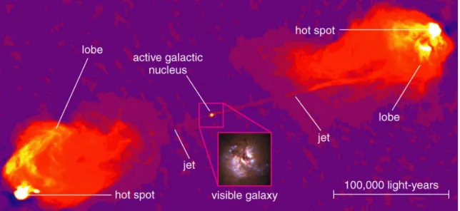
Figure 1.1:

VLA image of the 100 kpc long jets in Cygnus A, an AGN with twin relativistic jets that eventually shock against the intergalactic medium producing lobes of synchrotron emission. Credit: NRAO, Pearson Education, Inc., publishing as Addison Wesley.

phologies. One of the main classification treats of AGN is the division between AGN with strong radio emission and AGN with weak or no radio emission. Another im- portant AGN classifiers are the one related to the presence or absence of broad lines in the spectrum and the bolometric luminosity. The weak radio emitters are classi- fied as Seyfert 1 or Seyfert 2 galaxies, depending on the presence of broad or narrow emission lines. Radio galaxies, quasars or blazars are different categories of strong radio emitters with increasing luminosity.

A fraction of AGN, mainly those with intense radio emission, manifest well col- limated outflows (jets) ejected from the nucleus and dissipating their energy in the large-scale radio lobes. The bulk of radio emission originates from the jets and lobes, and so the presence of these structures is the main factor distinguishing between radio-loud and radio-quiet AGN. Jets can propagate over extremely large distances, reaching up to more than 1 Mpc. At large scales, two types of radio galaxies (FR I and FR II) are identified, depending on their morphological features [Fanaroff and Riley, 1974]. The FR II are characterized by powerful edge- brightened double lobes with prominent hot-spots and tend to be found in less dense environments, while the FR I have radio emission peaking near the nucleus, have rather edge-darkened lobes and frequently inhabit more dense environments. Cygnus A shown in Fig. 1.1 is a classic FR II radio source. Jets in quasars often appear to be one-sided, although in several objects a second or counter hot-spot is observed. In Blazars, the jets are very compact and one- sided.

Several unification schemes have been proposed to explain this observed diversity

[Blandford and Rees, 1978; Urry and Padovani, 1995]. A lot of differences can be

explained with changing the viewing angle, i.e., the angle between the orientation

of the jet and accretion disk and our line of sight. The central regions of many AGN appear to contain obscuring material, probably in the form of gas and dust.

Depending on the orientation, our line of sight would cross materials moving at different speed, explaining the different signature in the width of the emission lines.

Superluminal motions have also been detected in some AGN jet [Rees, 1966] which can only be explained if relativistic speed is observed with small viewing angle.

Another effect of a relativistic jet is that the radiation is strongly beamed along the jet direction. In this context Blazars and Quasars are objects viewed with a smaller viewing angle compare to radio galaxy, explaining the apparent larger intensity, and the one- sidedness of their jet. The various different class of AGN are summarized in Fig. 1.2.

1.2 Imaging an AGN jet

The electromagnetic radiation from AGN is spread over a wide range of frequencies from radio to γ-rays. The accretion disk emits mainly thermal optical-UV radiation, while the jets emits non-thermal synchrotron and inverse Compton radiation. The synchrotron radiation is emitted by relativistic charged particles when they are radi- ally accelerated through magnetic fields. At kpc scales the jet emission peaks at low frequencies while the inner parsec region mainly emits at higher frequencies reaching up to optical, X-ray, and even gamma-ray regimes. An AGN jet is thus best observed in the radio regime. It should also be noted that some close by AGN jets have also been successfully observed in the optical and X-ray regime using the Hubble Space Telescope (HST) and the Chandra space telescope.

The limited resolution offered by single dish radio telescopes accelerated the de-

velopment of radio interferometer consisting of an array of telescopes. Using this

technique, it is possible to reach angular resolution inversely proportional to the

largest distance between two sub-components of the array. Each two elements of

an interferometer form an interferometric baseline and measure, at every instant,

a particular interferometric visibility, which is one component of the Fourier trans-

form of the spatial distribution of the brightness of the observed object. The total

combination of all baseline visibilities comprise a combined measurement of an in-

terferometric response of the observed object in the Fourier domain, also called u-v

plane. Through inverse Fourier transform, it is thus possible to recover an image of

the observed object. The procedure of creating images from these measurements is

called aperture synthesis. For this operation to succeed it is important to measure as

many visibilities as possible. This can be done by increasing the number of elements

in the array, and designing the layout of the array so that it maximize the number of

different baselines. Radio interferometers also take advantage of the rotation of the

Earth to increase the number of baseline orientations. Several non-linear deconvolu-

tion algorithms have been developed to be able to produce images with a relatively

sparse and irregular set of baselines. The CLEAN algorithm [H¨ogbom, 1974] and the

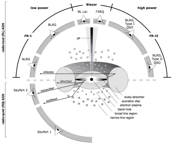
Figure 1.2:

Schematic representation of the current AGN unification model. The division between radio-loud (upper part) and radio-quiet AGN (lowe part) can be explained by the presence or absence of a powerful jet responsible for most of the radio emission. Obscuring material around the black hole may explain the different emission lines characteristic.

Relativistic beaming effect plays also a role in the observed luminosity of radio-loud AGN.

Credit: Beckmann, Shrader.

Maximum Entropy Method are two popular method in radio astronomy.

In the early days of radio interferometry, the baseline length was limited to few

kilometers. The three-elements One-Mile Telescope completed in 1964 was able to

achieve a resolution of 80

at 408 MHz. An advantage of observations at radio wave-

lengths in comparison to measurements at shorter wavelengths is that the telescopes

output comprising both the amplitude (voltage) and phase of the incoming electro-

magnetic wave, can be easily transfered from one point to another through cables, and

can even be recorded for later processing. This possibility led to the rapid increase

of baselines length, and the development of the technique of Very Long Baseline In-

terferometry (VLBI). By combining telescopes separated by thousands of kilometers,

it was possible to reaches angular resolution of smaller than one milliarcsecond of

arc. The Very Large Baseline Array (VLBA), a dedicated VLBI instrument oper-

ated by the National Radio Astronomy Observatory (NRAO) has been in operation

since 1993. It uses ten 25-meter telescopes spanning up to 8000 kilometers across the United States, and it is able to reach a resolution of 0.17 mas at 47 GHz. The European VLBI Network (EVN) operated by the European Consortium for VLBI is able to combine up to 20 individual telescopes spread across the entire globe, includ- ing some of the world’s largest and most sensitive radio telescopes, making it the most sensitive VLBI array in the world. A good review about the effort and develop- ments that made this instrument a reality can be found in Porcas [2009]. Increasing further the angular resolution requires either longer baselines or observing at higher frequency. Using space-based VLBI antennas such as HALCA [Hirabayashi et al., 1998] and RadioAstron [Kardashev et al., 2013], resolution as high as 10 µas can be reaches. Extending VLBI observations to millimeter and sub-millimeter wavelengths is another approach to achieve ultra hight angular resolution, with up to 50 µ as at 3 mm wavelengths (86 GHz) [see Krichbaum et al., 2013, for details].

1.3 Motivation and organization of the work

The high resolution imaging capability offered by radio interferometry is key for our understanding of relativistic jets. Detailed analysis of the jet structure and evolution on sub-parsec to parsec scales can bring unique insights on the mechanisms involved in their formation, collimation and acceleration [Hada et al., 2011; Nakamura and Asada, 2013]. Investigations of jet stability and notably the structural pattern changes caused by Kelvin-Helmholtz instability pave the way to determining the physical parameters governing the flow [Lobanov and Zensus, 2001; Hardee et al., 2005]. Relativistic jets are also a prominent source of high energy emission and hence investigations of jets can serve as a laboratory for high energy plasma physics [Kirk and Duffy, 1999]. Structural variability can be analyzed in connection with high energy flares, thus probing the location and origin of high energy emission [Schinzel et al., 2012].

The task of producing an image from VLBI observations is challenging. Recon- structing an image from visibilities in the Fourier domain is essentially an inverse problem that is ill posed and will not have a unique solution. The combined contin- ued progress in non-linear deconvolution techniques and increased sensitivity of radio telescopes have considerably improved the quality of radio interferometric images.

Maps of several prominent relativistic jets shows transversely resolved structure and contain a wealth of morphological and dynamical information. Efficient extraction of this information is of paramount importance for understanding the physics and evolution of these objects. The algorithms and methods currently employed for this purpose (such as Gaussian model fitting) often use simplified approaches to describe the structure of resolved objects. Automated (unsupervised) methods for structure decomposition and tracking of structural patterns are needed for this purpose to be able to treat the complexity of structure and large amounts of data involved.

This dissertation is primarily dedicated to development, testing, and application of

pioneering methods for automated decomposition and tracking of two-dimensional structural patterns in extragalactic relativistic jets.

The dissertation is divided in five main parts. In Chapter 2, we provide a brief review on our current understanding on jets physics. In Chapter 3, we introduce a new wavelet-based image segmentation and evaluation (WISE) method for multiscale decomposition, segmentation, and tracking of structural patterns in astronomical images. In Chapter 4, WISE is tested against simulated images of relativistic jets.

In Chapter 5, the jets in 3C 273, 3C 120 and 3C 111 are analyzed using data from the Monitoring Of Jets in Active galactic nuclei with VLBA Experiments (MOJAVE) program. Finally, in Chapter 6, we will present the results of the kinematic analysis of the innermost part of the M87 jet.

Throughout this thesis, we assume a cosmology with H

= 70 km s

Mpc

,

Ω

= 0.3 and Ω

= 0.7

Jet physics

Presence of astrophysical outflows have been found in diverse objects with remarkably large range of scales, masses, and physical types. The jets produced by active galactic nuclei (AGN) are probably the most powerful of this category. Direct or indirect indication of jets have also been found in microquasars, X-ray binaries, Young Stellar Objects (YSO) and Gamma Ray Bursts (GRB). Despite the large diversity of these objects, they all share two main elements that are critical for the formation of jets:

a compact, rotating, and magnetized central engine, and matter accreting towards this central source. Different models have been invoked to explain the formation and propagation of jets. This chapter presents a brief summary of the basic concepts of magnetic outflows that is the most commonly accepted model that explain the observed structure and properties of the different categories of jets.

2.1 Central engine and accretion disk

The first key element common in all extragalactic jets is a compact object. In the case of AGN, this is the Super Massive Black Hole ( ∼ 10

–10

M

) , while it could be the white darf, neutron star or smaller black hole in X-ray binary, the collapsing star in GRB events or the protostars in YSO. Strong gravitational forces associated with the central object result in accretion surrounding material onto it, which is typically accompanied by formation of an accretion disk. The creation of an accretion disk provides the energy supply, in the form of kinetic energy of the infailling matter, necessary for the formation of the large scale jet. The configuration of this system is illustrated in Fig. 2.1

A Black Hole (BH) is characterized by its mass m, and its angular momentum

J or, equivalently, dimensionless BH spin a = J/J

[Tchekhovskoy, 2015]. An

important reference point of the black hole description is the event horizon surface,

defined as the boundary in through which matter and light can fall inward towards

the black hole but can never re-emerge [Beckmann and Shrader, 2012]. In the case of

a non-rotating black hole (a = 0), this region occurs at the so-called Schwarzschild

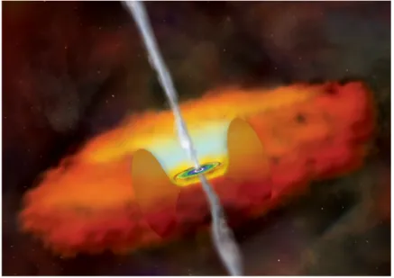
Figure 2.1:

Artist view of a black hole surrounded by an accretion disk of hot gas and torus of cooler gas and dust. (Credit: NASA/CXC/M.Weiss).

radius:

R

= 2Gm

c

(2.1)

and gravitational field is described in terms of the Schwarzschild metric. In the case of rotating black hole (0 < a < 1), the Kerr metric is used, and the event horizon is defined as:

R

= R

2 (1 + √

1 − a

) (2.2)

This basic difference between rotating and non-rotating black hole is actually an important one. The BH spin is an additional source of energy that can be extracted through the so-called Penrose process. Additionally, the spin will define the in- nermost stable circular orbit (ISCO), which correspond to the accretion disk inner radius. It varies from r

= 6R

for a non rotating black hole to r

= 1R

for a maximally rotating black hole [Bardeen et al., 1972].

The full detail of the mechanism of accretion onto the central black hole is still not clear. Several models have been invoked to explain the observed accretion properties.

The Bondi accretion consider an approximated spherically symmetrical accretion flow. Following Beckmann and Shrader [2012], in this model the black hole will accrete matter at an approximate rate:

M ˙

= πR

ρv (2.3)

with ρ and v the accretion wind density and velocity, and R

the effective capture radius that is approximatively found using the escape velocity of the central engine:

R

= 2Gm

v

(2.4)

The actual amount of matter accreted by the central object is then defined in term of Bondi accretion rate ˙ M

= α M ˙

, with α representing the efficiency of the accretion and is model dependent.

This model allows us to determine the basic physical conditions in the vicinity of an accreting object. However the accretion flow is unlikely to be spherically symmetrical close to the black hole, and we expect more a disk-shaped structure. A model for a thin, viscous disk (or alpha disk) has been first proposed by Shakura and Sunyaev [1973]. Different models of Advection Dominated Accretion Flow (ADAF) have also been invoked to explain the radiative inefficiently of some low luminosity AGN [Narayan et al., 1998].

2.2 Jet launching

In the canonical picture of the disc accretion, the formation of a collimated outflow can be viewed as an inevitable consequence of the accretion. There has to be a loss of momentum in order to have accretion due to momentum conservation law, and the transport of matter above the disk in the form of a wind is an efficient way to extract angular momentum. Analytic modeling and numerical simulation of such systems have found that a condition for the creation of such wind is the presence of a large scale magnetic field. The magnetic field in the vicinity of the black hole can be advected inwards by the accreting matter in the disk [Blandford and Payne, 1982], or alternatively it can be generated locally by a disk dynamo [Tout and Pringle, 1996].

Close to the disk, the field lines are anchored in the disk, and will co-rotate with it.

Considering a cylindrical coordinate system (z, r, φ), with z the axis of rotation, and (r, φ) the plane of the disk (see Fig. 2.2), the magnetic field can be decomposed into a poloidal, B

= B

(r, z)ˆ r + B

(r, z)ˆ z, and toroidal component, B

= B

(r, z) ˆ φ.

The poloidal field will dominate close to the disk, and can be written as [Vlahakis, 2015]:

B

= 1

r ∇ Ψ(r, z) × φ ˆ (2.5)

with Ψ(r, z) the so-called poloidal magnetic flux function. Field lines are defined as lines of constant flux function on the (z, r) plane.

In the standard Blandford & Payne model, the energy source of the wind is the kinetic energy of the rotating disk, with the most powerful component of the jet, accelerated to high bulk Lorentz factor at large distance, being launched in the inner part of the accretion disk, close to the ISCO. In this region we can approximate the rotation to be Kelperian, and the corresponding angular velocity Ω can be written as:

Ω =

s mG

r

(2.6)

with r

the radius in the plane of the accretion disk of the field line, which we can call

launching location. In a similar way, the jet can be launched from the magnetosphere

Accretion disk

Black hole Magnetosphere Field lines

Figure 2.2:

Illustration of the field lines configuration near the black hole. Field lines are either anchored in the accretion disk or in the magnetosphere of the rotating black hole.

The two important parameters determining the power of the jet are the angular velocity of the central object or accretion disk Ω, and the magnetic flux Ψ. The distance between two field lines

is an essential parameter of the acceleration and collimation of the jet after the fast magnetosconic point.

of a rotating black hole, extracting the rotational energy of the central engine through the Penrose process. Blandford and Znajek [1977] first demonstrated the viability of this hypothesis and found that the effective angular velocity of the corresponding field line would be:

Ω

' 0.5 Ω

= 0.5 ac

2r

(2.7)

These two mechanisms of energy extraction are illustrated in Fig. 2.2 which shows field lines anchored in both the magnetosphere and the accretion disk. In the first case, the field line angular velocity will be constant Ω = Ω

, while in the second case, it will decrease with the distance of the anchored point to the central engine.

The field angular velocity define a critical point called the light cylinder radius at r

= r/(Ωc).

In the model of magnetic outflows that we are adopting here, a magneto- centrifu- gal mechanisms initiate the launching and acceleration [Blandford and Payne, 1982].

Magnetic pressure dominates in the low density and gas pressure of the atmosphere

of the disk. While the flow co-rotates with the disk, it is unrestricted by the magnetic

forced along the field lines [Spruit, 2010]. The flow experiences a centrifugal force

accelerating it along them, much as if it were carried in a set of rotating rigid tubes

anchored in the disk. At a distance called the Alfv´en point (AP), close to the light

cylinder in the case of relativistic flow, co-rotation of the field lines and the flow

ceases, and the field starts lagging behind, developing a significant toroidal compo-

nent. This transition can be seen in Fig. 2.3 where the Lorentz factor, velocity and

magnetic field of a typical relativistic magnetic flow are plotted along the distance

from the central engine. The acceleration by centrifugal forces will also halt at this

transition point, and the magnetic pressure of the toroidal magnetic field will drive

further acceleration through hoop stress forces up to another critical point, the fast

2 4 6 8 10 12

γ,γσ

µ^1/3

γ γσ

0.2 0.4 0.6 0.8 1.0

β

βφ

βp

10⁻⁵ 10⁻⁴ 10⁻³ 10⁻² 1010⁻¹⁰ 10¹ 10²

B

10⁰ 10¹ 10²

r(rlc) FMP

RLC R₀

B_φ Bp

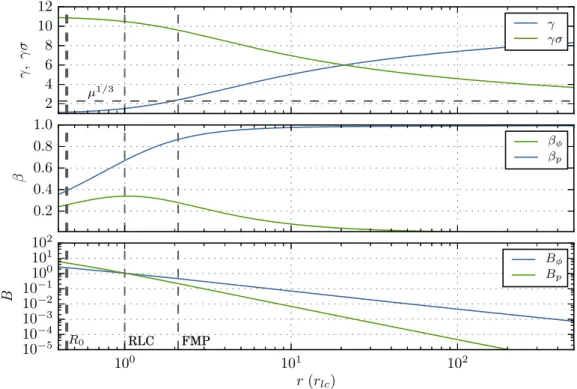
Figure 2.3:

Typical example of evolution of a magnetic flow with distance from the central engine. Top panel: the Lorentz factor (blue) increases at the expense of the magnetic energy (green). Equipartition between kinetic and Poynting energy is achieved around

20r

. Middle panel: The toroidal velocity (green) is maximum at the light cylinder radius and then decrease. Bottom panel: The poloidal magnetic field (green) dominates at the inlet of the flow and decrease like

1/r

, while the toroidal magnetic field (green) decrease like

∼

1/r and start to dominate around the light cylinder. In the three panels, the launching location (R

), fast magnetosonic point and light cylinder are indicated.

magnetosonic point (FMP).

2.3 Jet acceleration and collimation

The total specific energy (matter + electromagnetic) µ and the angular momentum L are conserved along a field line. In the approximation of cold ideal magnetohydro- dynamics MHD flow these can be expressed following Vlahakis [2015]:

µ(Ψ) = γ − rΩB

cη (2.8)

L(Ψ) = γrv

− crB

η (2.9)

where γ is the bulk Lorentz factor of the flow, v

is the toroidal component of the velocity and η represents the distribution of mass flux at the inlet of the flow:

η = 4πγρ

β

c

B

(2.10)

The ratio of the magnetic (or Poynting) to kinetic energy flux can be introduced by the magnetization parameter:

σ = µ − γ

γ (2.11)

At the inlet, the flow is non-relativistic (γ

∼ 1) and is therefore Poynting dominated.

It has been demonstrated [Vlahakis, 2015] that at the fast magnetosconic point the flow reaches a Lorentz factor γ

∼ µ

(also see Fig. 2.3). In fact, if the field lines were radial the flow would stop accelerating before this point, slowly reaching its maxmimum Lorentz factor γ

∼ µ

[Michel, 1969]. The additional acceleration that would explain the observed high Lorentz factor (γ ∼ 10), and kinetic dominated flow [Sikora et al., 2005] strongly depends on the configuration of the field lines, and on their collimation. Li et al. [1992] found that acceleration can continue if the flow expansion is such that the distance between the field lines δl increase faster than the cylindrical distance r (see Fig. 2.2), which constitutes the so-called “magnetic noozle”

mechanisms. After the FMP, acceleration and collimation are concurrent, explaining at the same time the observed Lorentz factors and opening angles of parsec scale of AGN jets. This process is slow, and both numerical simulation [Komissarov et al., 2007] and observations have shown that acceleration can indeed continue up to large distances (z ∼ 10

–10

R

), achieving equipartition between Poynting and kinetic energy around z

∼ 10

R

.

2.4 Instabilities

Different types of plasma instability can develop in relativistic flows, with Current driven (CD) instability and Kelvin-Helmholtz (K-H) instability being the most com- monly expected ones.

The kink mode of the CD instability occurs when the jet have developed a strong toroidal magnetic field [Mizuno et al., 2012]. It is one of the most dangerous instabil- ities as it will act on the center of mass of the fluid, and is hence able to disrupt the outflow (see Panel C in Fig. 2.4). It might, however, be a necessary process as it is suspected to be one of the mechanisms able to transfer electromagnetic energy into plasma energy. As an MHD instability, it operates mainly in the Poynting dominated part of the jet.

The K-H instability is a consequence of velocity shear in a fluid. In AGN jets, it is expected to grow at the transition layer between the jet and the ambient medium and can be modeled by a pressure perturbation:

p

= exp(i(kz + nφ − wt)) (2.12)

A B

C

Figure 2.4:

Example of instabilities that are known to develop in AGN jets. Simulation of linearly growing elliptical body mode and helical mode of the Kelvin-Helmholtz instability is shown in panel A and B respectively (Credit: P. Hardee). In panel C, we reproduce simulation of the kink mode of the Current Driven instability from

[2012].

with k and n the longitudinal and azimuthal wavenumber respectively, and w the frequency. K-H instability can be classified by their wavenumber into different modes.

The pinch (n = 0), helical (n = 1), and elliptical (n = 2) modes are expected to be most prominent in supersonic, relativistic flows [Lobanov and Zensus, 2001], each having a surface and multiple body mode (see Panel A and B in Fig. 2.4). Contrary to the CD instability, it will operate mainly in the kinetic energy dominated part of the jet.

2.5 Relativistic effects

AGN jets are fast, relativistic flows with high Lorentz factors, which makes a variety of relativistic effects affecting the observed manifestations of the jets. If a source of radiation is moving at a velocity near the speed of light along a direction close to the observer’s line of sight, the time interval between the emission of two successive photon as measured in the observer’s frame is reduced, and the source appears to move faster than it actually does [Blandford and Konigl, 1979]. If β = v/c is the intrinsic speed of the flow, and θ the viewing angle, the apparent velocity β

is obtained using:

β

= β sin(θ)

1 − β cos(θ) (2.13)

Relativistic Doppler effect will also alter the observed radiation of the source.

As a consequence of time dilation and aberration of light, the radiation will be

concentrated within a cone with an angle of 1/γ with respect to the flow direction,

with γ describing the Lorentz factor of the plasma. The observed intensity will be

boosted if observed at a viewing angle θ inside this cone (i.e., θ < 1/γ), while it will

0 2 4 6 8 10 12 14

βapp

0 2 4 6 8 10 12 14

γ θ= 5^◦ θ= 10^◦ θ= 15^◦ θ= 20^◦

0 2 4 6 8 10 12

δ

0 2 4 6 8 10 12 14

γ θ= 5^◦ θ= 10^◦ θ= 15^◦ θ= 20^◦

Figure 2.5:

Example of relativistic effect with implication on the apparent velocity (left panel) and observed radiation (right panel). The apparent velocity

and Doppler factor

is computed for different viewing angle

and Lorentz factor

of the flow.

be de-boosted outside this cone. The corresponding Doppler factor δ is:

δ = 1

γ(1 − β cos(θ)) (2.14)

The resulting dependences of the apparent velocity and Doppler boosting on γ

and θ are illustrated in Fig. 2.5. Blazars with viewing angles θ ∼ 5° are strongly

boosted and can display large super-luminal motions. In misaligned blazars, like the

jet in M87 with viewing angle θ ∼ 20 ° , the apparent velocity will be smaller and

the jet appearance can also be affected by de-boosting of material with very high

Lorentz factors.

Wavelet-based Image

Segmentation and Evaluation

Part of the work presented in this chapter is published in Mertens and Lobanov [2015]

3.1 Introduction

The steady improvements of the dynamic range of astronomical images and the ever- increasing complexity and detail of astrophysical modeling bring a higher demand on automatic (or unsupervised ) methods for characterizing and analyzing structural patterns in astronomical images.

Several of the approaches developed in the fields of computer vision and remote- sensing to track structural changes [cf. Yuan et al., 1998; Doucet and Gordon, 1999;

Arulampalam et al., 2002; Sidenbladh et al., 2004; Doucet and Wang, 2005; Myint et al., 2008] either require oversampling in the temporal domain or rely on multiband (multicolor) information that underlies the changing patterns. This renders them difficult to be used in astronomical applications that typically focus on tracking changes in brightness in a single observing band, which are monitored with sparse sampling, and in which the structural displacements between individual image frames often exceed the dimensions of the instrumental point spread function (PSF).

Astronomical images and high-resolution interferometric images in particular of- fer very limited (if any) opportunity to identify “ground control points” or to build

“scene sets”, as employed routinely in remote-sensing and machine-vision applica-

tions [cf. Djamdji et al., 1993; Zheng and Chellappa, 1993; Adams and Williams,

2003; Zitov´a and Flusser, 2003; Paulson et al., 2010]. Structural patterns observed

in astronomical images often do not have a defined or even preferred shape, which

is an aspect relied upon in a number of the existing object recognition algorithms

[e.g., Agarwal et al., 2003]. Astronomical objects normally do not feature sufficiently

robust edges that would warrant applying the edge-based detection and classification

commonly used in object-recognition methods [Belongie et al., 2002]. In addition,

astronomical images often feature partially transparent optically thin structures in

which multiple structural patterns can overlap without full obscuration, which makes these images even more difficult to analyze using the algorithms developed for the purposes of remote-sensing and computer vision. Because of these specifics, auto- mated analysis and tracking of structural evolution in astronomical images remains very challenging, and it requires implementing a dedicated approach that can address all of the main specific characteristics of astronomical imaging of evolving structures.

Currently, structural decomposition of astronomical images normally involves simplified supervised techniques based on identification of specific features of the structure [e.g., ridge lines, Hummel et al., 1992; Lobanov et al., 1998; Bach et al., 2008], analysis of image-brightness profiles [cf. Lobanov and Zensus, 2001; Lobanov et al., 2003] , or fitting the observed structure with a set of predefined templates (e.g., two-dimensional Gaussian features [Pearson, 1999; Fomalont, 1999]). Two- dimensional cross-correlation has been attempted only in very few cases [ e.g., Biretta et al., 1995; Walker et al., 2008], each time requiring manual segmentation of images, which imposed strong limitations on the number of structural patterns that could be tracked.

In some particular situations, for instance, in images of extragalactic radio jets, distinct structural patterns cover a variety of scales and shapes from marginally resolved brightness enhancements caused by relativistic shocks embedded in the flow [Zensus et al., 1995; Unwin et al., 1997; Lobanov and Zensus, 1999] to thread-like patterns produced by plasma instability [Lobanov, 1998a; Lobanov and Zensus, 2001;

Hardee et al., 2005]. In the course of their evolution, most of these patterns may rotate, expand, deform, or even break up into independent substructures. This makes template fitting and correlation analysis particularly challenging, and simultaneous information extraction on multiple scales and flexible classification algorithms are required.

Deconvolution algorithms [cf. H¨ogbom, 1974; Clark, 1980] extended to multi- ple scales [e.g., Cornwell, 2008] might in principle be able to recover such complex structures. However, comparing structures imaged at different epochs is difficult as a result of the general non-uniqueness of the solutions provided by deconvolution and because of an obvious need to group parts of the solution together to describe structures that are substantially larger than the image PSF.

A more robust approach to automatize identification and tracking of structural

patterns in astronomical images can be provided by a generic multiscale method

such as wavelet deconvolution or wavelet decomposition [cf. Starck and Murtagh,

2006]. While wavelets are typically applied for image- denoising and compactifica-

tion, they provide all ingredients necessary to decompose the overall structure in an

image into a robust set of statistically significant structural patterns. This chapter

explores the wavelet approach and presents a wavelet-based image segmentation and

evaluation (WISE) method for structure decomposition and tracking in astronomical

images. The method is based on combining wavelet decomposition with watershed

segmentation and multiscale cross-correlation algorithms to treat temporal sparsity

of astronomical images, multiscale structural patterns, and their large displacements between individual image frames.

The conceptual foundations of the method are outlined in Sect. 3.2. An algorithm for segmented wavelet decomposition (SWD) of structure into a set of statistically significant structural patterns (SSP) is introduced in Sect. 3.3. A multiscale cross- correlation (MCC) algorithm for tracking positional displacements of individual SSP is described in Sect. 3.4. Finally, a stacked cross correlation (SCC) method used to determine velocities components in stratified flow is developed in Sect. 3.5.

3.2 Wavelet-based image structure evaluation (WISE) algorithm

3.2.1 Wavelet transform

The wavelet transform is a time-frequency transformation that decomposes a square- integrable function, f(x), by means of a set of analyzing functions, ψ

(x), obtained by shifts and dilations of a spatially localized square-integrable wavelet function ψ(x), so that

ψ

(x) = 1

√ a ψ

x − b a

(a 6 = 0) , (3.1)

where a > 0 is the scale parameter and b is the position parameter. The Morlet- Grossman definition [A. Grossmann, 1984] of the continuous wavelet transform for a one-dimensional function f(x) ∈ L

(R), the space of all square-integrable functions, is:

W (a, b) = 1

√ b Z

f (x)ψ

x − b a

dx . (3.2)

Different discrete realisations of the wavelet transform exist [Mallat, 1989; Starck and Murtagh, 2006]. In the analysis presented here, the ` a trou wavelet [Holschneider et al., 1989; Shensa, 1992] is employed. The ` a trou wavelet transform has the ad- vantage of yielding stationary, isotropic, and shift-invariant transformation which is well-suited for astronomical data analysis applications [Starck and Murtagh, 2006].

Different scaling functions can be used with this transform [Unser, 1999]. The choice of the scaling function is guided by the specific properties of the image and the infor- mation required to be extracted from the image [Ahuja et al., 2005]. In the following, we have used the B-spline scaling function (also called the triangle function).

For the purpose of this work, we consider digital astronomical images as sampled data c

(k) defined as a scalar product (computed at locations k) of a function f (x) (sky brightness distribution, convolved with the instrumental point-spread-function) with a scalar scaling function φ(x), yielding

c

(k) = h f (x), φ(x − k) i . (3.3)

This operation corresponds to application of a low pass filter to a continuous function.

The scaling function φ is chosen to satisfy the dilation equation 1

2 φ 1

2

= X

l

h(l)φ(x − l) . (3.4)

In this expression, h is a discrete low pass filter associated with the scaling func- tion. The smoothed data c

(k) at position k and a given resolution j, containing information of f (x) on spatial scale > 2

is given by

c

(k) = 1 2

f(x), φ( x − k 2

, (3.5)

which is obtained by computing the convolution c

(k) = X

m

h(m)c

(k + 2

l) . (3.6) The wavelet coefficients w

(k) containing information on spatial scales between 2

and 2

are then given by the difference between two consecutive scale resolutions:

w

(k) = c

(k) − c

(k) . (3.7) Equations (3.4) and (3.7) gives the expression of the wavelet function for this particular transform:

1 2 ψ

1 2

= φ(x) − 1 2 φ

1 2

. (3.8)

This expression can be easily extended to a two-dimensional case. Applied to an image, it produces a set w

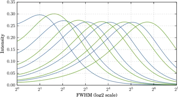
(k, l) of resolution-related views of the image which are called wavelet scales. The concept of spatial wavelet scale plays a role similar to that of a spatial frequency (cf., Fourier transformation): small scales correspond to high frequency and large scales to low frequency. In Figure 3.1, this relation is illustrated for a one-dimensional case by plotting the relative sensitivity of different wavelet scales to fiducial spatial scales represented through brightness distribution described by a Gaussian profile with the respective full width at half maximum (FWHM).

3.2.2 Conceptual structure of WISE

To characterize the structure and structural evolution of an astronomical object, the

imaged object structure needs to be decomposed into a set of significant structural

patterns (SSP) that can be successfully tracked across a sequence of images. This

is typically done by fitting the structure with predefined templates [such as two-

dimensional Gaussians, disks, rings, or other shapes deemed suitable for representing

particular structural patterns expected to be present in the imaged region; Fomalont,

1999; Pearson, 1999] and allowing their parameters to vary. It is clear, however, that

0.0 0.1 0.2 0.3 0.4 0.5

Intensity

1 2 4 8 16 32

FWHM (log2 scale)

Scale 1 Scale 2 Scale 3 Scale 4 Scale 5 Scale 6

Figure 3.1:

Relation between scales of a wavelet transform and spatial scales represented by the FWHM of a Gaussian profile. The individual curves represent the relative sensitivity of a given wavelet scale for recovering a Gaussian feature with a given FWHM. The FWHM for which a wavelet scale is the most sensible, characterized by a peak of intensity, is shown in abscissa. Wavelet transfrom is performed using the triangle scaling function.

for a robust structural decomposition made without a priori assumptions, the generic shape of these patterns must be allowed to vary as well. To ensure this, a method is needed that can automatically identify arbitrarily shaped statistically significant structural patterns, quantify their significance, and provide robust thresholding based on the significance of individual features.

The multiscale decomposition provided by the wavelet transform [Mallat, 1989]

makes wavelets exceptionally well-suited to perform such a decomposition, yielding

an accurate assessment of the noise variation across the image and warranting a ro-

bust representation of the characteristic structural patterns of the image. To further

increase the robustness of the method, the multiscale approach is extended here to

object detection, similarly to the methodology developed for the multiscale vision

model [MVM; Ru´e and Bijaoui, 1997; Starck and Murtagh, 2006] in related work

on object and structure detection [Men’shchikov et al., 2012; Seymour and Widrow,

2002]. By combining these features, we have developed a new, wavelet-based image

structure evaluation (WISE) algorithm that is aimed specifically at the structural

analysis of semi-transparent, optically thin structures in astronomical images. The

method involves segmented wavelet decomposition (SWD) of individual images into

arbitrary two-dimensional SSP (or image regions) and subsequent multiscale cross-

correlation (MCC) of the resulting sets of SSP. A detailed description of the method

is given below.

3.3 Segmented wavelet decomposition

The segmented wavelet decomposition (SWD) comprises the following steps to de- scribe an image structure by a set of SSP:

1. A wavelet transform is performed on an image I by decomposing the image into a set of J sub-bands (scales), w

, and estimating the residual image noise (variable across the image).

2. At each sub-band, statistically significant wavelet coefficients are extracted from the decomposition by thresholding them against the image noise.

3. The significant coefficients are examined for local maxima, and a subset of the local maxima satisfying composite detection criteria is identified. This subset defines the locations of SSP in the image.

4. Two-dimensional boundaries of the SSP are defined by the watershed segmen- tation using the feature locations as initial markers.

These steps essentially combine the MVM approach with watershed segmenta- tion [Beucher and Meyer, 1993] and a two-level thresholding for the purpose of yielding a robust SSP identification procedure that would improve the quality of subsequent tracking of SSP that have been cross-identified in a sequence of images of the same object.

The SWD decomposition delivers a set of scale-dependent models (SDM), each containing two-dimensional features identified at the respective scale of the wavelet decomposition. The combination of all SDM provides a structure representation that is sensitive to compact and marginally resolved features as well as to structural pat- terns much larger than the FWHM of the instrumental PSF in the image. Moreover, individual SSP identified at different wavelet scales are partially independent, which allows for spatial overlaps between them and can be used to improve the robustness and reliability of detecting structural changes by cross-correlating multiple images of the same object.

3.3.1 Determination of significant wavelet coefficients

As has been discussed above, the wavelet transform of a signal produces a set of zero

mean coefficient values w

at each scale j. To extract significant wavelet coefficients

and filter out the noise, a threshold, τ

, is determined by requiring | w

| ≥ τ

for the

significant coefficients. The determination of τ

depends on the noise characteristics

in the image and a false discovery rate (FDR) . For the purpose of this work, it is

assumed that the image noise is Gaussian. Techniques exists to handle other types

of noise, for example using the Anscombe transform for Poisson noise. We refer

to Starck and Murtagh [2006] for a complete review of noise treatment in wavelet

analysis of images.

The wavelet transform does not change the Gaussian nature of the noise and hence the noise can be characterized at each scale of its wavelet decomposition by a zero mean and a standard deviation σ

. This property can be used for relating the desired noise threshold τ

to σ

by setting τ

= k

σ

and requiring the significant coefficients to satisfy the condition | w

(x, y) | ≥ k

σ

. Choosing k

= 3 gives an FDR = 0.002. The application of the threshold condition yields a denoised map for each wavelet scale:

m

(x, y) =

( w

(x, y) if | w

(x, y) | >= kσ

0 otherwise . (3.9)

In order to determine σ

from the standard deviation of the noise of the original image σ

, the standard deviations σ

are calculated for each scale of the wavelet decomposition of simulated Gaussian-noise data with σ

≡ 1. We then use the linearity of the wavelet transform to obtain σ

from the relation σ

= σ

σ

[Starck and Murtagh, 1994].

An estimate of σ

can be obtained using one of the several techniques available for this purpose. If a noise map can be accessed, σ

is provided simply by calculating the standard deviation of the entire map or of the relevant areas in the map. In other situations, k-sigma clipping or Median Absolute Deviation (MAD) estimation [Starck and Murtagh, 2006] can be applied to assess the noise properties in the image and obtain an estimate of σ

.

3.3.2 Localization of significant structural patterns

A maximum filter is used to identify putative positions of SSP at each scale of the wavelet decomposition. The filter comprises applying the morphological operation of dilation with a structuring element of a desired size. The location of a local maxima occurs when the output of this operation is equal to the original data value. This defines a list of local maxima, H

, at the scale j:

H

= { (x, y) : dilation(w

(x, y)) = w

(x, y) } . (3.10) The shape and size of the chosen structuring element affect the smallest separation of two detected local maxima. For our specific application, we use a diamond structur- ing element of a size that matched the scale at which it is applied; with the minimum size of two pixels. Each of the lists H

is clipped at a specific detection threshold, ρ

. This is done recalling that for Gaussian noise, the detection level is proportional to σ

, hence ρ

= k

σ

can be set. For successful detection thresholding, the condition k

≥ k

must be satisfied (with k

= 4–5 typically providing good thresholds).

The threshold clipping can be applied for defining F

as a group of significant feature locations:

F

= { f = (x, y) : (x, y ) ∈ H ∧ | w

(x, y) | ≥ k

σ

} , (3.11)

and these locations can be used for subsequently defining SSP in the image.

0 1 2 3 4 5 6 7

wj(x)

0 20 40 60 80 100 120 140 160

x(pixel) fa

SSP a

fb

SSP b τ =ksσj

ρ=kdσj

Figure 3.2:

Schematic illustration of the method used for SSP localization, applied to a one-dimensional case. The local maxima (triangle marker) are located using the maximum filter and the SSP are associated with each of the local maxima by applying the watershed flooding algorithm. In this example the SSP “a” associated with the position

is defined by a region between 25 pix and 82 pix.

3.3.3 Identification of significant structural patterns

An SSP is defined as a 2D region of enhanced intensity extracted at a given wavelet scale. To determine the extent and shape of individual SSP associated with signif- icant local maxima, image segmentation needs to be performed. The segmentation relates each local maximum to a range of surrounding pixels that can be considered part of this local intensity enhancement. The map of significant coefficients, m

, is used for that purpose. The borders between individual regions are determined from the common minima located between the adjacent regions. This is achieved by wa- tershed flooding [Beucher and Meyer, 1993]. The watershed flooding earns its name from effectively corresponding to placing a “water source” in each local minimum and “flooding” the image relief from each of these “sources” with the same speed.

The moment that the floods filling two distinct catchment basins start to merge, a dam is erected to prevent mixing of the floods. The union of all dams constitutes the watershed line. Figure 3.2 illustrates the application of the watershed segmentation in a one-dimensional case.

The watershed segmentation is performed on − m

at all scales j with F

as “water sources”, or markers. Each local maximum f

of F

gives a region s

defined as

s

(x, y) =



 

 

m

(x, y ) if (x, y) is inside the watershed line of f

;

0 otherwise .

(3.12)