High frequency VLBI observations of galactic and extragalactic sources

(1)

High frequency VLBI observations of galactic and extragalactic sources

INAUGURAL-DISSERTATION

Erlangung des Doktorgradeszur

der Mathematisch-Naturwissenschaftlichen Fakultät der Universität zu Köln

vorgelegt von Christoph Rauch Bergisch Gladbach, Deutschlandaus

Köln 2016

(2)

der Universität zu Köln

1. Referent: Prof. Dr. Andreas Eckart 2. Referent: Prof. Dr. Anton Zensus Tag der Promotion: 21.04.16

Erscheinungsjahr: 2016

Diese Dissertation ist auf dem Universitäts Publikations Server der Universität Köln unter http://kups.ub.uni-koeln.de/ elektronisch publiziert.

(3)

Universität zu Köln

Abstract

by Christoph Rauch for the degree of Doctor rerum naturalium

The radio source Sagittarius A* (Sgr A*), which is commonly associated with the super-massive black hole in the Galactic Center, oers the largest angular dimension of an active galactic nucleus and, therefore, the best opportunity to study the underlying physics of these objects. While orbital parameters of nearby stellar sources have proven its existence beyond reasonable doubt, its energy production mechanism is still uncertain.

Sgr A* shows intensity outbursts, referred to as ares, which occur on time scales ranging from 7-10 minutes (sub-ares) to 1-2 hours (main-ares). Several models are currently under investigation, that can explain the observable properties of the quiescent and aring state of Sgr A*. The observed amplitudes and time scales of near-Infrared (NIR) and X-ray ares are consistent with expected values of an expansion with an adiabatic cooling mechanism. Alternatively, a hot spot model, is also capable of reproducing the observed parameters. Such a feature is, in analogy to the solar coronal mass ejection, formed by ux ropes, which are capable of rapidly expelling material, if their equilibrium stability is lost. Other models explain these ux excesses by a temporary accretion disc with a short time jet or a mixed Jet-advection-dominated accretion ow.

A set of observable parameters, that can be used to discriminate between the currently proposed models, are the full-width at half max (FWHM) Gaussian size of the emission region, the absolute position of Sgr A*, its symmetry, as well as time delays and time scales of its ares. Relativistic magnetohydrodynamic simulations predict an almost constant size and shape of the emission region.

Therefore, a change of its FWHM size, position or symmetry would point towards a jet or hot spot model. The expected changing source size and/or asymmetry are caused by an adiabatically expanding, orbiting or spatially constant, o- center component. In addition to this, the ares of Sgr A* show correlated ux excesses at dierent wavelengths ranging from NIR/X-ray to radio frequencies.

The time delay found between these frequencies oers the opportunity to analyze physical properties that arise at dierent radii, because individual observing bands measure distinct radial regions.

The subject of this thesis is to discriminate between the described aring models of Sgr A*. Three six-hour Very Long Baseline Interferometry (VLBI) observations at 43 GHz have been performed on May 16 - 18 2012 in parallel

(4)

are observed on May 17 triggered the VLBI observation of this date, which shows a are peaking at 1.41 Jy, delayed by (4.5±0.5)h. This increasing ux density is apparently accompanied by a changing source structure, that can best be modeled by a central emission region with a weak secondary component of 0.02 Jy at about 1.5 mas under 140^◦ (east of north).

Dierent cleaning methods have been tested, which lead to consistent maps of Sgr A* showing an o-center component in both polarizations. Symmetry-tests, based on analysis of closure phases, residual noise maps and simulated articial data sets, improved the robustness of this two component model. Furthermore, positions acquired from phase referencing analysis oer large error limits and have to be considered as constant.

The observed position of the secondary component, which is still aected by interstellar scattering, oers speeds of (0.4±0.3)c for the presented time delay of (4.5±0.5)h between the NIR and 7 mm are. This time lag represents the velocity between dierent radial regions around the black hole mapped by the individual frequencies. Relating this and several other delays, provided by the current literature, to theoretical intrinsic source sizes and interpolating them to a common NIR/X-ray center, results in a radial velocity prole of Sgr A* that appears to be accelerating towards the outermost regions.

The complexity of required calibration and technical observing inaccuracies does not allow to completely exclude weather or other random observational eects to be the cause of the extended source structure, but we have shown, that with most careful cleaning eorts, this two component structure stays robust and is most probable a real data feature. The complete quantity of indications of a secondary component during the aring states of Sgr A* are within one to two sigma. The consistent set of hints towards a two component structure excludes the hot spot model, because of its spatial dimension, and points towards the existence of a temporary jet anchored at Sgr A*.

(5)

UNIVERSITÄT zu Köln

Zusammenfassung

von Christoph Rauch zur Erlangung des Doktorgrades

Doctor rerum naturalium

Das im Allgemeinen mit der Radioquelle Sagittarius A* (Sgr A*) assoziierte super-massereiche Schwarze Loch im galaktischen Zentrum bietet die gröÿte räumliche Dimension eines aktiven Galaxiekerns und daher die beste Möglichkeit die zugrunde liegenden physikalischen Prozesse dieser Objekte zu untersuchen.

Während Orbitalparameter benachbarter Sterne dessen Existenz jenseits begrün- deter Zweifel bewiesen haben, ist der vorhandene Energieproduktionsmechanis- mus noch nicht vollständig geklärt.

Sgr A* zeigt Intensitätsausbrüche, die auch als Flares bezeichnet werden, auf Zeitskalen von 7-10 Minuten (Sub-Flares) bis zu 1-2 Stunden (Main-Flares). Ver- schiedene Modelle werden derzeit diskutiert, welche fähig sind, die beobacht- baren Eigenschaften der inaktiven und aktiven Phasen von Sgr A* zu erklären.

Die Amplituden und Zeitskalen der Nahinfrarot- (NIR) und Röntgen-Flares sind konsistent mit einer adiabatisch gekühlten Expansion. Alternativ kann auch ein Hot-Spot Modell diese Parameter reproduzieren. Solch eine Struktur wird, in Analogie zum solaren koronalen Massenauswurf, durch Flussröhren geformt, welche fähig sind Material rapide auszuwerfen, sobald sie ihre Gleichgewichtssta- bilität verlieren. Andere Modelle erklären die beobachteten Intensitätsausbrüche durch eine temporäre Akkretionsscheibe und einen kurzzeitigen Jet sowie durch ein Konglomerat aus Jet und advektions-dominierter Akkretion.

Die Halbwertsbreite (FWHM) der Emissionsregion, die absolute Position von Sgr A*, dessen Symmetrie sowie die Zeitunterschiede und Zeitskalen der Flares bieten eine Reihe beobachtbarer Parameter, die herangezogen werden können, um zwischen den derzeitigen Modellen zu unterscheiden. Relativistische Mag- netohydrodynamik Simulationen sagen eine beinahe konstante Gröÿe und Form der Emissionsregion voraus. Daher würde eine Veränderung der FWHM, Po- sition oder Symmetrie auf ein Jet oder Hot-Spot Modell hindeuten. Die er- wartete Veränderung der Quellgröÿe und/oder Asymmetrie werden durch eine adiabatisch expandierende, auÿerhalb des Zentrums gelegene, statische oder es umkreisende, Komponente hervorgerufen. Auÿerdem zeigen die Intensitätsaus- brüche korrelierte Flussexzesse zwischen verschiedenen Wellenlängen, die sich über den NIR-/Röntgenstrahlungs- bis zum Radiobereich erstrecken. Die Zeit- verzögerung zwischen verschiedenen Frequenzen bietet die Möglichkeit physika- lische Eigenschaften auf unterschiedlichen Radien zu analysieren, da einzelne

(6)

Diese Dissertation beschäftigt sich mit dem Thema, zwischen den beschriebe- nen Modellen der aktiven Phasen von Sgr A* zu unterscheiden. Drei sechsstündige Langbasisinterferometrieaufnahmen (VLBI) bei 43 GHz wurden zwischen dem 16. und 18. Mai 2012, parallel zu NIR-Aufnahmen des Very Large Telescopes (VLT), durchgeführt. Ein NIR-Flare am 17. Mai triggerte die VLBI-Aufnahmen dieses Datums, die eine um (4.5±0.5)h verzögerte ansteigende Flussdichte bis auf einen Wert von 1.41 Jy detektierten. Dieser Flare geht anscheinend mit einer Veränderung der Quellstruktur einher, welche am besten durch eine zentrale Emissionsregion und eine schwache sekundäre Komponente von 0.02 Jy, die sich unter einem Winkel von 140^◦ (östlich) in einer Entfernung von 1.5 mas bendet, modelliert werden kann.

Verschiedene Bildgenerierungsmethoden wurden geprüft und weisen konsistente Karten von Sgr A* mit einer sekundären Quelle abseits des Zentrums in bei- den Polarisationen auf. Die Belastbarkeit dieses Zweikomponentenmodells wurde getestet, indem die Quellsymmetrie anhand von Closure Phasen, Rauschresiduen und simulierten Datensätzen untersucht wurde. Des Weiteren zeigen die Posi- tionen, die durch Phasenreferenzierungsanalysen erhalten wurden, hohe Fehler- grenzen und müssen daher als konstant angesehen werden.

Die beobachtete Position der sekundären Komponente, welche durch inter- stellare Streuung beeinträchtigt ist, zeigt Geschwindigkeiten von(0.4±0.3)c für eine Zeitverzögerung von (4.5±0.5)h zwischen NIR- und 7 mm-Flares. Diese Verzögerung repräsentiert die Geschwindigkeit zwischen den verschiedenen Ra- dien um das Schwarze Loch, welche durch die unterschiedlichen Frequenzen de- tektiert werden. Bringt man diese und andere, in der derzeitigen Literatur erwäh- nten, Zeitverzögerungen in Relation zu der theoretischen intrinsischen Quellen- gröÿe und interpoliert sie in Bezug auf ein gemeinsames NIR-/Röntgenstrahlungs- Zentrum, so ergibt sich ein radiales Geschwindigkeitsprol von Sgr A*, welches eine Beschleunigung hin zu den äuÿersten Regionen aufzeigt.

Die Komplexität der Kalibrations- und technischen Aufnahmeungenauigkeiten erlaubt es nicht, Wetter oder andere zufällige Aufnahmeeekte auszuschlieÿen.

Es kann aber behauptet werden, dass selbst bei einer mit höchstmöglicher Acht- samkeit durchgeführten Bildgenerierung die Zweikomponentenstruktur belast- bar bleibt und daher höchstwahrscheinlich ein reales Datenmerkmal ist. Die Gesamtheit der Hinweise auf eine sekundäre Komponente während der aktiven Phasen von Sgr A* liegt innerhalb von ein bis zwei Sigma. Diese konsistente Reihe von Anzeichen für eine Zweikomponentenstruktur schlieÿt ein Hot-Spot- Modell, aufgrund seiner räumlichen Ausdehnung, aus und deutet auf die Existenz eines kurzzeitigen Jets mit Ursprung in Sgr A* hin.

(7)

A scientist is happy, not in resting on his attainments but in the steady acquisition of fresh knowledge.

Max Planck, 1858 - 1947

(8)

(9)

Acknowledgements

I thank Prof. Dr. A. Zensus to open the possibility for me to work in the VLBI group and granting the funding. I am grateful for his eective and positive supervision during the thesis advisory committee and several personal meetings, which were not only scientically fruitful, but also provided organizational help.

I would like to express my gratitude to Prof. Dr. A. Eckart for supervising me during my Diploma thesis and Dissertation over the last years. Thank you for giving me the impression of always being welcome and solving my many questions with impressive facility.

I would like to thank Prof. Dr. E. Ros for introducing me into the astonishing world of radio astronomy and for always having an open door. Not only for his very constructive scientic advices, but also for his permanent good mood while answering my many questions, which created a pleasant and productive working atmosphere.

Furthermore, I thank Dr. T. P. Krichbaum for his time spent and scientic input which kept me on track towards generating real and reliable results. Even during periods of peaking work loads he found the time to help me with his knowledge in the data reduction and imaging processes as well as technical aspects, that were mandatory for this work.

And of course I want to thank Dr. K. Muºi¢ for her participation in the thesis advisory committee meetings and her scientic input for the publication of this thesis.

I want to thank Banafsheh Shahzamanian for providing us with the NIR light curve on which the VLBI observations have been triggered, that lead to interesting results.

Dr. Ru-Sen Lu has earned my thanks for sharing his knowledge with us and providing additional ideas.

And of course my oce mates Dr. Biagina Boccardi, Dr. Sebastian Kiehlmann and Dr. Vassilis Karamanavis, who managed to be a reliable source of information and joy, that was just one look over the shoulder away.

I also want to thank Dr. Je Hodgson for correcting our publication and further improving its scientic results.

The whole VLBI group also deserves to be thanked for their advices and interesting topics during our meetings.

Further acknowledgements go to the participants of conferences at the physics de- partments of the Christian-Albrechts-university in Kiel and the Nicolaus Copernicus

(10)

Special thanks go to my family for their support and love during this time.

This work was supported through a stipend from the International Max Planck Re- search School (IMPRS) for Astronomy and Astrophysics at the Universities of Bonn and Cologne.

(11)

List of Figures

1.1 Observable universe in logarithmic scale. The image is centered on the sun with the Big Bang at its edge. Source: Pablo Carlos Budassi/Wikimedia Commons. 8 1.2 Binding energy per nucleon as a function of their total number contained in

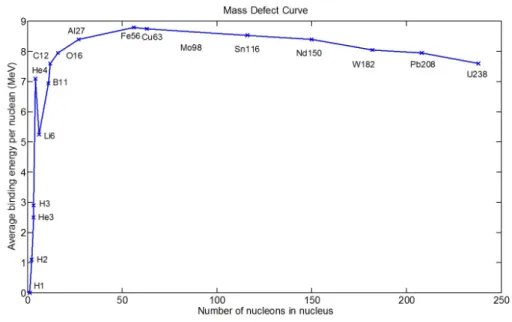
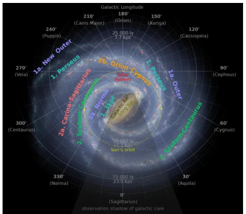
the nucleus. Source: Lewis(2008) . . . . 9 1.3 Overview of the Laniakea supercluster. Source: Tully et al.(2014) . . . 10 1.4 Milky Way map with position of the solar system. The obscuring dust in

the Galactic Bar casts an observational shadow on all sources behind it at optical/NIR wavelengths. Source: NASA / JPL-Caltech / R. Hurt (SSC- Caltech). . . . 11 1.5 Composite image of the Galactic Center taken at Infrared (red, Mission:

Spitzer Space Telescope), Optical (yellow, Mission: Hubble Space Telescope) and X-ray (blue, Mission: Chandra X-ray Observatory). Instrument: IRAC.

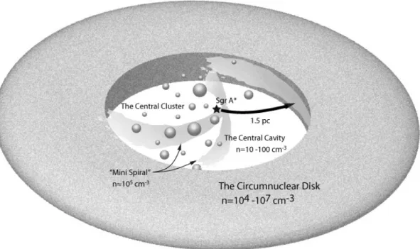
Source: NASA, ESA, CXC, SSC, STScI, JPL-Caltech . . . 12 1.6 Schematic view of the Galactic Center. Relative positions of Sgr A* and the

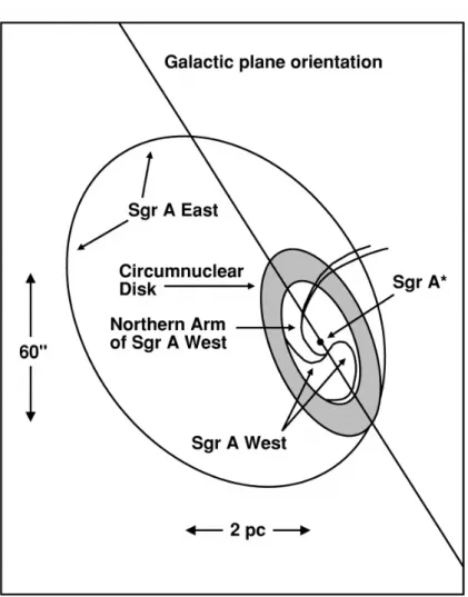
central cluster within the central cavity are shown within the circum nuclear disk. Source: (Goto et al.,2013).. . . 13 1.7 Schematic overview of the Sgr A complex. Source: Bagano et al.(2003) . . . 14 2.1 Orbit of S2 between 1992 and 2013 with respect to Sgr A*. Source: MPE-IR

Galactic Center Group (Genzel, R.) and UCLA group; http://www.mpe.mpg.

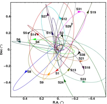
de/369216/The_Orbit_of_S2. . . . 19 2.2 Illustrative orbits of stars in the central arcsecond around Sgr A*. The coor-

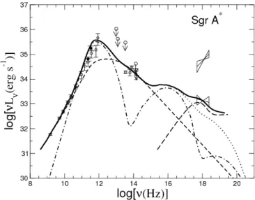
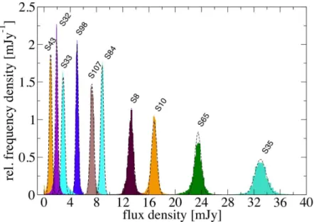
dinate system origin is dened as the position of Sgr A*. Source: (Gillessen et al.,2009).. . . 19 3.1 Observed spectrum of Sgr A*. Source: (Yuan et al.,2003) . . . 22 3.2 Normalized ux density histogram of ten non-variable calibrator sources in the

Galactic Center. The dashed lines represent Gaussian ts of the distribution.

Source: (Witzel et al.,2012). . . . 23 3.3 Illustration of the hot spot model proposed by (Yuan et al.,2009). A ux rope

can be formed as a result of the foot point motion and subsequent magnetic reconnection. This feature can be ejected and results in a are. Source: (Yuan et al., 2009). . . . 27 4.1 Atmospheric opacity as a function of wavelength. Source: NASA/IPAC . . . . 30 4.2 Schematic overview of the receiver setup of a radio telescope. . . . 30 4.3 Schematic overview of the time delays between individual telescopes. B~ is the

vector along the baseline of individual telescopes and~s is the vector of unity in the direction of the observed source.. . . 32 4.4 Illustration of(u, v)-plane and(l, m)-coordinates. Schematic overview, accord-

ing toMiddelberg & Bach(2008). . . . 33

(14)

Bottom left: (u, v)-track of a telescope array forming several baselines observing at multiple frequencies. Bottom right: Detailed view of a multi-frequency (u, v)-track segment. Source: (Middelberg & Bach, 2008) . . . 34 5.1 Telescope sites of the VLBA. All antennas oer a diameter of 25 m and form

an array with a maximum baseline of about 8000 km. Source: NRAO.. . . 40 5.2 Earth's atmospheric layers. The most signicant eects on astronomical ob-

servations arise from the amount of electrons in the ionosphere (ne) and the quantity of water vapor contained in the troposphere. Source: Singh et al.(2004) 42 5.3 Global map of the total electron content in the ionosphere taken on 16 Dec

2015. The color scale on the right represent total electron content units in 10¹⁶m⁻². Source: NASA Jet Propulsion Laboratory.. . . 44 5.4 VLBA antenna (KP) gain as a function of time observed on May 17 2012. This

plot shows the eect of changing elevations on the amplitudes of Sgr A*. . . . 45 6.1 Uncalibrated amplitudes of NRAO 530 for the baseline KP-LA in LCP as a

function of frequency for two subbands (IFs). Time range: 9:08:28 to 9:10:28 h UT.. . . 53 6.2 Bandpass calibrated amplitudes of NRAO 530 for the baseline KP-LA in LCP

as a function of frequency for two subbands (IFs). Vector averaged cross-power spectrum. The amplitude scale has been changed compared to 6.1 in order to better show the residual small uctuations. Time range: 9:08:28 to 9:10:28 h UT. 53 6.3 Uncalibrated phases of NRAO 530 for the baseline KP-LA in LCP as a function

of frequency for two subbands (IFs). Time range: 9:08:28 to 9:10:28 h UT. . . 56 6.4 Fringe tting results (delay-corrected solution) of the baseline KP-LA in LCP

for NRAO 530 as a function of frequency for two subbands (IFs). Time range:

9:08:28 to 9:10:28 h UT. . . . 56 6.5 Uniformly weighted LCP contour images of Sgr A*. The correspond-

ing dates and peak ux intensities are: (a) May 16 2012 8-12 h UT, 1.11 Jy/beam. (b) May 17 2012 6-12 h UT, 1.34 Jy/beam. (c) May 18 2012 8-12 h UT, 1.17 Jy/beam. All maps have been convolved with a common beam of 2.74×1.12 mas at 1.76^◦. The plotted contour levels represent 1.73%, 3.46%, 6.93%, 13.9%, 27.7%, 55.4% of the peak ux intensity (taken from Rauch et al.(2016)). . . . 59 6.6 ^{(u, v)}-coverage of Sgr A* on May 17 2012 (6-12 h UT). Available stations FD,

KP, LA, and PT (taken fromRauch et al. (2016)). . . . 61

(15)

7.1 7 mm and NIR light curves of Sgr A* on May 17 6-12 h UT 2012. (a) NIR Ks-band (2.2µm) light curve, produced by combining 0^◦ and 90^◦ polarization channels (taken fromShahzamanian et al.(2015)). (b) DFT of the 7 mm ux of Sgr A* (red) and the calibrator NRAO 530 (blue) (taken fromRauch et al.(2016)). (c) Detrended DFT of Sgr A* at 7 mm (taken fromRauch et al. (2016)). (d) 7 mm light curve provided by the intensities of the two-hour maps of Sgr A* (see Fig. 7.2, taken from Rauch et al. (2016)). Obtained uxes are based on delta-component maps (red) and model tting (blue), while the errors are derived from to the formal error of 1.7% found for the calibrator NRAO 530. Systematic errors in the order of ∼18% are not included, which should be corrected in the calibration process. . . . 64 7.2 Time segmented two hour LCP contour images of Sgr A* observed on May 17

2012. (a) May 17 6-8 h UT. (b) May 17 7-9 h UT. (c) May 17 8-10 h UT. (d) May 17 9-11 h UT. (e) May 17 10-12 h UT. Map parameters can be found in Tab. 7.1 (taken fromRauch et al. (2016)). . . . 66 7.3 Model ts of Sgr A* on May 17 2012 6-12 h UT for ve overlapping two-hour

segments. The time range of 8-10 h UT (c) is best tted by a two component model indicating an extended morphology during the aring state. (a) May 17 6-8 h UT. (b) May 17 7-9 h UT. (c) May 17 8-10 h UT. (d) May 17 9-11 h UT.

(e) May 17 10-12 h UT. Summarized map parameters can be found in Tab. 7.2 (altered fromRauch et al. (2016)). . . . 67 7.4 Cross-correlation coecient of the NIR and 7 mm light curves during the aring

phase of Sgr A* on May 17 2012. . . . 68 7.5 Closure amplitudes for Sgr A* on May 16 (red) and May 17 (blue). . . . 70 7.6 Clean map of Sgr A* on May 17 2012 (8-10 h UT) in RCP. The map has been

convolved with a beam of 2.74×1.12 mas at 1.76^◦ and plotted with contour levels at 1.73%, 3.46%, 6.93%, 13.9%, 27.7%, and 55.4% of the peak ux density of 1.5 Jy/beam (taken fromRauch et al.(2016)). . . . 72 7.7 Illustration of a closure triangle. . . . 73 7.8 Closure Phases and standard deviation levels for all closure triangles of

Sgr A* in LCP on May 17 6-12 h UT (altered fromRauch et al.(2016)).

(a) FD-KP-PT, (b) FD-KP-LA, (c) FD-LA-PT, (d) KP-LA-PT. All phases are plotted with the standard errors provided by difmap. . . . . 75 7.9 Closure Phases and standard deviation levels for all closure triangles of

Sgr A* in RCP on May 17 6-12 h UT. (a) FD-KP-PT, (b) FD-KP-LA, (c) FD-LA-PT, (d) KP-LA-PT. All phases are plotted with the standard errors provided by difmap. . . . 76 7.10 Closure Phases and standard deviation levels for all closure triangles of

Sgr A* in LCP on May 16 8-12 h UT. (a) FD-KP-PT, (b) FD-KP-LA, (c) FD-LA-PT, (d) KP-LA-PT. All phases are plotted with the standard errors provided by difmap. . . . 77

(16)

(c) FD-LA-PT, (d) KP-LA-PT. All phases are plotted with the standard errors provided by difmap. . . . 78 7.12 Angular size of Sgr A* in mas derived from central circular model t shown in

Fig. 7.3 as a function of time. For the time range of 8-10 h UT only the central component has been considered. . . . 82 7.13 Radial plot of Sgr A* during its period of strongest aring activity on May

17 2012. The colors of the tted models correspond to the time ranges 8-10 h UT (red), 9-11 h UT (orange) and 10-12 h UT (blue) (taken fromRauch et al.

(2016)).. . . 83 7.14 Three-day map of Sgr A* (Fourier deconvolution of all observed visibilities).. . 84 7.15 Residual map of Sgr A* on May 17 8-10 h UT showing a slight indication of

asymmetry along the NW/SE axis. The scale shows higher ux values as darker areas. . . . 85 8.1 Illustration of a jet, showing the regions observable by dierent wavelengths.

Even though this illustration shows a quasar, dierent frequencies will equally map dierent radial regions of the environment of Sgr A*. Source: (Marscher, 2005) . . . 90 8.2 Scaled map of the shells spanned by the observations listed in Tab. 8.1. . . . . 94 8.3 Time delay vs intrinsic size of the data in Tab. 8.5 plotted with a linear scale.

The time delay of this thesis andRauch et al.(2016) is plotted in blue, while red points are measurements directly linked to the X-ray/NIR core and green points represent interpolated data points. . . . 96 8.4 Time delay vs intrinsic size of the data in Tab. 8.5 plotted with a logarithmic

scale. The time delay of this thesis andRauch et al.(2016) is plotted in blue while red points are measurements directly linked to the X-ray/NIR core and green points represent interpolated data points. . . . 97 8.5 Velocity vs intrinsic size of the data in Tab. 8.5. The velocity derived from

the time delay of this thesis and Rauch et al. (2016) is plotted in blue while red points are measurements directly linked to the X-ray/NIR core and green points represent interpolated data points. . . . 97 8.6 Velocity vs intrinsic size of the data in Tab. 8.5 plotted with a logarithmic

scale. The velocity derived from the time delay of this thesis andRauch et al.

(2016) is plotted in blue while red points are measurements directly linked to the X-ray/NIR core and green points represent interpolated data points. . . . 99

(17)

List of Tables

4.1 Summary of VLBI surveys. Source: (Ros,2012) . . . 36 4.2 Observable parameters by VLBI. Source: (Ros,2012) . . . 37 6.1 Summary of agging applied to the dataset BE061 before calibration. KP and

MK had no failures. . . . 54 7.1 Observing times, peak ux and RMS noise values for all maps of May 17 pre-

sented in Fig. 7.2. All maps have been restored with a beam of (2.74×1.12) mas at 1.76^◦. The plotted contour levels represent 1.73%, 3.46%, 6.93%, 13.9%, 27.7%, 55.4% of the peak ux intensity. . . . 65 7.2 Summary of all map parameters for Fig. 7.3. All maps have been restored

with a beam of (2.74×1.12) mas at1.76^◦. The plotted contour levels represent 1.73%, 3.46%, 6.93%, 13.9%, 27.7%, 55.4% of the peak ux intensity. . . . 65 7.3 Closure phase values of Sgr A* for all closure triangles on May 16 and 17 (taken

from Rauch et al.(2016)). . . . 75 7.4 Simulated closure phase values of Sgr A* for all closure triangles on May 17

8-10 h UT (taken fromRauch et al. (2016)). . . . 80 7.5 Summary of residual noise values, if convolved with the 3 day delta component

model on May 16 and 17.. . . 83 7.6 Summary of phase referencing positions of Sgr A* on May 17. The error

amounts to 0.3 mas for all measurements. . . . 87 8.1 Summary of time delays at dierent frequencies for Sgr A*. . . . 92 8.2 Summary of velocities at dierent frequencies for Sgr A*. . . . 93 8.3 Intrinsic angular size of Sgr A* as a function of the wavelength. Derived ac-

cording to Falcke et al.(2009). . . . 95 8.4 Relative intrinsic angular shell size and mean velocity values for the areas

mapped by dierent wavelengths of the observations summarized in Tab. 8.1 Sgr A*. Sizes and velocities have been derived according toFalcke et al.(2009). 96 8.5 Data points interpolated from Tab. 8.1 Sizes and velocities have been derived

according toFalcke et al.(2009). . . . 98

(18)

(19)

Nomenclature

Abbreviations

ADAF Advection-dominated accretion ow

ADIOS Advection-dominated inow-outow solutions AGN Active galactic nuclei

AO Adaptive optics

BR Brewster

CARMA Combined Array for Research in Millimeter Astronomy CDAF Convection-dominated accretion ows

CONICA Coudée Near Infrared Camera CXC Chandra X-ray Observatory

DC Direct current

Dec. Declination

DFT Direct Fourier transform

EDAF Ejection-dominated accretion ow ESA European Space Agency

EVN European VLBI Network

FD Fort Davis

FFT Fast Fourier transform FWHM Full-width-at-half-maximum

HN Hancock

IC Inverse Compton

ICRF International Celestial Reference Frame IF Intermediate frequency

IRAC Infrared Array Camera

ITRF International Terrestrial Reference Frame JCMT James Clerk Maxwell Telescope

JPL-Caltech Jet Propulsion Laboratory at California Institute of Technology

KP Kitt Peak

LA Los Alamos

LCP Left-handed circular polarization (counter-clockwise) LO Local oscillator

MK Mauna Kea

MOJAVE Monitoring of Jets in Active Galactic Nuclei with VLBA Experiments

NACO NAOS and CONICA

NAOS Nasmyth Adaptive Optics

NASA National Aeronautics and Space Administration

NIR Near-Infrared

NL North Liberty

NRAO National Radio Astronomy Observatory

(20)

OV Owens Valley

PSF Point-spread-function

PT Pie Town

Quasar Quasi-stellar radio source QSO Quasi-stellar object R.A. Right ascension

RCP Right-handed circular polarization (clockwise) RFI Radio frequency interference

RIAF Radiatively inecient accretion ow

SC St. Croix

SED Spectral energy distribution SEFD System equivalent ux density Sgr A* Sagittarius A*

SMBH Super-massive black hole SMT Submillimeter Telescope SNR Signal to noise ratio

SSC Synchrotron + synchrotron self-Compton

SSC-Caltech Spitzer Space Center at California Institute of Technology STScI Space Telescope Science Institute

TANAMI Tracking Active Galactic Nuclei with Austral Milliarcsecond Interferometry TEC Total electron content

VIPS VLBA Imaging and Polarimetry Survey VLBA Very Long Baseline Array

VLBI Very Long Baseline Interferometry VLT Very Large Telescope

(21)

Used Symbols

a Angular momentum per unit mass A_ij Visibility Amplitude

A~_ij Additive baseline errors AV Extinction magnitude

b Digitization loss or normalization coecient B~ Baseline

B|| Parallel magnetic eld strength B¯ij Bandpass response matrix β power spectrum exponent βapp Apparent speed

c Speed of light or constant

C_n² Refractive index structure constant Γ Lorentz factor

D diameter

D¯_ij Polarization leakage matrix

δ Declination

δi phase error of the equipment at i.

δ_var Variability Doppler factor J¯ij Antenna voltage pattern matrix

Eν Sum of all monochromatic waves emitted by sources at a frequency ν E_ν^∗ Complex conjugate ofE_ν(~r)

F[f(x)] Fourier transform of a function f(x) F¯ij Ionospheric eect matrix

G Gravitational constant gi Voltage gain

G_i Conversion gain factor G¯_ij Electronic gain matrix

γ power law exponent or loop gain value η fringe moduli function

η_s Electronic losses Iν Intensity a frequencyν

J Angular momentum

J_i Corrupting factor

J¯ij Observational eects operator

k Wave number

K Normalization function Ki Antenna sensitivity

θ Angle

θ₀ Isoplanatic angle θint Intrinsic angular size θ_obs Observed angular size

(22)

Direction cosines pointing at source λ Wavelength

m Mass or direction cosines pointing at source or polarization level M Unit mass

M¯_ij Multiplicative baseline errors N Number of positions or stations ne Number of electrons

n_i Noise term

ν Frequency

∆ν Observing bandwidth

ξ_ij phase of the Fourier transform at baseline ij p Pressure

P¯ij Parallactic angle matrix

R Radius

Q, U Stokes Parameter of liner polarization

~

ri Observer location R_s Schwarzschild radius S Flux density

~s Unit vector towards source s_i Signal of a source

t Time

T Temperature

T¯_ij Tropospheric eects matrix Tb Brightness temperature Ts System temperature τ Geometric time delay τacc Accumulation time

u, v Coordinates of the plane orthogonal towards the line of sight ((u, v)-plane)

v Speed

V Stokes parameter of circular polarization Vν Visibility function at frequencyν

Φ Phase

∆φ Misalignment angle of phase shift xi Signal of antenna i

χ Polarization angle

Ψ Opening angle or phase angel

dΩ Surface element of the celestial sphere

ω_i time variable phase rotation of scans at telescope i.

z Distance

(23)

Numerical Constants

π = 3.14159 1rad = 57.296degrees

Physical Constants

Speed of light c= 2.9979×10⁸m s⁻¹ Gravitational constant G= 6.670×10⁻¹¹N m²Kg⁻²

Astronomical Constants

Astronomical unit (1 AU) = 1.496×10¹¹m Parcec (1 pc) = 3.086×10¹⁶m Julian light year (1 ly) = 9.460730472×10¹⁵m Julian year (1 yr) = 3.15576×10⁷s Solar mass (1 M) = 1.989×10³⁰Kg

(24)

(25)

Chapter 1

The Galactic Center

The universe has formed between(13.796±0.029)and(13.813±0.038)Gyr ago, based on current cosmic microwave background measurements (Planck Collaboration XIII, 2015). After the fundamental particles formed during the very rst seconds, these condensed into protons, neutrons and electrons, the rst simple components of atoms.

At this early stage 10 s to 20 min after creation, the thermal energy was still very high and thus, the high velocity of electrons prevented them from being caught in the sphere of inuence of other particles, that already had synthesized the least complex nuclei of Hydrogen (1p, 0n), Helium (2p,2n) and Lithium (3p, 3-4n) through fusion processes. After the incident thermal energy has been mitigated (around3×10⁶years), the electrons could be captured by the nuclei and form the rst electrically neutral atoms.

A large volume of interacting particles shows the tendency to condense into lamen- tary structures consisting of small scale clumps at the positions of density irregularities.

These gravity seeds will then start to gather more material by collision and gravitational attraction, forming, due to an initial rotation, spinning compact objects, that extract excessive matter in form of jets along the axis of least resistance (rotation axis). After the system has reached equilibrium state this process usually forms rotating spheroids with a central massive core like planets, stars or elliptical galaxies (E0-6 type). This process can to some extend be found on many astronomical scales, ranging from the large scale Galaxy clusters, over Galaxies, down to solar systems. This evolution shows that all Galaxies contain a very massive core and while stellar black holes can be formed, depending on their initial size, for masses above 1.5−3 M Bombaci (1996), it is logical to assume that most, if not all galactic nuclei contain a black hole, like Sgr A*, which is the main topic of this thesis (e.g.,Richstone et al. 1998;Gebhardt et al. 2000; Ferrarese & Merritt 2000; Gültekin et al. 2009; Seth et al. 2014). Figure 1.1shows a logarithmic illustration of the current picture of the universe up to the Big Bang. The current observable universe, dened by the maximum traveling range of light since the cosmological expansion, spreads over 28.5 Gpc.

The high density during the early stages of the universe, emphasizes creation of very massive objects. Therefore, after rst clumping of matter into large laments, the earliest created objects are assumed to be massive galaxies, quasars and population III stars. The strong radiation originating from these objects was capable of ionizing the surrounding material around 350×10⁶years ago. Within these high mass objects, many stars starting to fuse matter into more complex elements. Iron atoms are the end of this fusion chain, because it oers the highest bounding energy per nucleon (see Fig.1.2, left part) and thus, is found in the core of stellar or planetary objects

(26)

Figure 1.1: Observable universe in logarithmic scale. The image is centered on the sun with the Big Bang at its edge. Source: Pablo Carlos Budassi/Wikimedia Commons.

(27)

9

Figure 1.2: Binding energy per nucleon as a function of their total number contained in the nucleus. Source: Lewis(2008)

and their primordial stages. The evolution of some of these stars into a super nova created additional elements such as Uranium, which is capable of creating the remaining presently existing elements by nuclear ssion processes (right part of Fig. 1.2).

Our host galaxy, the Milky Way, is located in the, so called, Local Group of galaxies and oers a decentralized picture of our extended denition of home. At larger scales, this group is part of the Laniakea cluster (see Fig. 1.3), which is centered around a gravitational anomaly, called the Great Attractor (R.A.: 10h32m, Dec.: −46^◦00') at a distance of (45-50) Mpc (Mieske et al.,2005). While our solar system is located about 10-20 pc above the Galactic plane in the Orion-Cygnus arm, a relatively low density region of a normal barred spiral galaxy (see Fig. 1.4), the distance of∼8 kpc towards its center yields a∼26000 ly long path of possible electromagnetic aberration for the optical radiation originating in this region (see also Chap. 3). Observations of the Galactic Center are limited by obscuring dust and gas that aects electromagnetic radiation passing through it. It's a challenging task to overcome this hurdle at optical/NIR frequencies and it was not possible to gain high angular resolution images of this region until observational methods advanced to a state, that made it possible to detect ne structures and objects (see Fig. 1.5).

This extinction has its strongest eect close to the Galactic Center. Radio, infrared and X-ray wavelengths can pass this veil less aected and are, therefore, the best wavelengths to study the Galactic Center. This is also true for all sources located behind the Galactic Center, which casts an observational shadow (see Fig. 1.4). The Galactic disk rotates clockwise as viewed from the galactic north at about 220 to 244 km s⁻¹ (Bovy et al., 2009; Gillessen et al., 2009), with a rotation curve ratio of 29 to 32 km s⁻¹kpc⁻¹ (Reid & Brunthaler, 2004; Reid et al., 2009; McMillan et al.,

(28)

Figure 1.3: Overview of the Laniakea supercluster. Source: Tully et al.(2014)

(29)

1.1. Nuclear Stellar Cluster 11

Figure 1.4: Milky Way map with position of the solar system. The obscuring dust in the Galactic Bar casts an observational shadow on all sources behind it at optical/NIR wavelengths.

Source: NASA / JPL-Caltech / R. Hurt (SSC-Caltech).

2010). This translates into a period of about 240 million years, making it necessary to deal with these observational obstacles in order to gain insights on the Galactic Center region and obscured sources at optical/NIR-wavelengths. The ability to observe the nucleus of the Galactic Center behind this dusty veil made it one of the most prominent subjects in astrophysics and the detection of a central super-massive black hole (SMBH) even further raised interest in this target. This thesis aims at gaining further insights on the physical processes of this very interesting source, which is a current concern of astronomical science.

1.1 Nuclear Stellar Cluster

The Galactic Center is a very complex area, containing a huge amount of distinct objects and gaseous streams. Figure 1.5 provides a nice overview of its complexity and the amount of features. Molecular clouds absorb a large part of its radiation and are, therefore, associated with the dark areas in this image. Within this region of high object density reside massive star clusters, supernova remnants and at a few parsecs the circum nuclear disk (see Fig. 1.6). The central objects within the Galactic Center can be decomposed into a nuclear bulge of1.4×10⁹M, covering the central hundreds

(30)

Figure 1.5: Composite image of the Galactic Center taken at Infrared (red, Mission: Spitzer Space Telescope), Optical (yellow, Mission: Hubble Space Telescope) and X-ray (blue, Mission:

Chandra X-ray Observatory). Instrument: IRAC. Source: NASA, ESA, CXC, SSC, STScI, JPL-Caltech

of parsecs, an enclosed stellar disc (radius: ∼ 230pc, scale height: ≤ 45pc) and a compact nuclear stellar cluster (NSC) (Launhardt et al.,2002). This NSC is assumed to inherit a high amount of star formation derived from its strong UV-radiation and stellar luminosity function. The attened NSC spreads over(4.2±0.4)pc (half-light or eective radius, enclosing half of the total emitted ux) with a mass of (2.5±0.4)×10⁷M

and is rotating in the same direction as the Galactic Center (Schödel et al.,2014). Its misalignment of∼10^◦ is currently assumed to be caused by individual accretion events during the time of cluster formation (Schödel et al.,2015).

Schödel et al. (2007) report, that the dense and clumpy molecular ring, called the circum nuclear disk, orbits the gravitational center an radius of∼1.6 pc with a velocity of ∼110 km s⁻¹ (Guesten et al., 1987; Jackson et al., 1993; Christopher et al., 2005).

Within this ring ionized gas forms three major streams, called the mini-spiral, which connects the disk with the central star cluster. NIR observations provide a clear view of the stars inside the mini spiral and currently provide, due to its proximity and angular size, the only observations of a cluster that can be resolved into individual stellar sources at milli-pc scales. The achievable detection limit only allows high magnitude stars at NIR wavelengths to be detected, that only account for about 1%of its total stellar population. These stars are mostly red/blue super-giants and all main sequence stars down to ∼2 M.

According toMeyer(2008a), one of the rst radio observations, oering the required observational precision and techniques to overcome the limiting obstacles, revealed the radio complex Sagittarius A which can be resolved into a supernova remnant (Sagit- tarius A East), an extended source (Sagittarius A West), which was identied with

(31)

1.1. Nuclear Stellar Cluster 13

Figure 1.6: Schematic view of the Galactic Center. Relative positions of Sgr A* and the central cluster within the central cavity are shown within the circum nuclear disk. Source:

(Goto et al.,2013).

the mini spiral and a very compact (<1⁰⁰), bright radio source Sagittarius A* (Sgr A*) with unique properties (see Fig. 1.7) (Balick & Brown, 1974). The latter source was discovered to be the counterpart of electromagnetic radiation released by hot plasma close to a SMBH of∼4.0×10⁶M(see Sect. 2.1). This source is the main science target of this thesis and Sgr A* will in the following refer to the black hole together with its narrow neighborhood up to the radii of detected electromagnetic radiation originating from the matter within the black holes immediate gravitational inuence. The focus of this work lies on the physical properties of this object and the theories that try to explain its energy production mechanism. This source has shown intensity outbursts that are discussed in detail in section3.2. Special emphasis is put on the models trying to explain this aring behavior.

(32)

Figure 1.7: Schematic overview of the Sgr A complex. Source: Bagano et al.(2003)

(33)

Chapter 2

Black Holes

The theory of black holes is an unconventional approach that needed great courage to propose and pursue such a groundbreaking idea. These must have been characteristics that John Michell (Michell,1784) and Pierre Simon Laplace (Laplace,1796) possessed when they introduced the idea of objects that provide such strong gravitational elds that are capable of conning objects and even electromagnetic radiation in their gravitational inuence. As with most discoveries, the idea of black holes needed the fortunate mind of an inspired scientist to create a mathematical framework for this theory, long before any experimental hints pointing towards the true existence of such objects in nature could be observed. Einstein (1916) provided, with his general relativity, an instrument to describe the theory andSchwarzschild(1916) found the rst mathematical solution for it. This mathematical framework and its success in the scientic community paved the way for many follow up theories, considering charged (Reissner,1916;

Nordström,1918), spinning (Kerr,1963) and both spinning plus charged (Newman et al.,1965) black holes.

Following the argumentation in Zamaninasab (2010a), the no hair theorem provides solutions of the Einstein-Maxwell equations in four space-time dimensions that can be uniquely characterized by three variables: mass, electric charge, and angular momentum. In a static case with a spherical symmetry, no angular momentum and no electric charge, the Schwarzschild metric (Schwarzschild,1916) can be used to describe the environment of a black hole. The additional consideration of electric charge of the mass is included in the formalism of the Reissner-Nordström metric (Reissner, 1916;

Nordström,1918). A more generalized description of the Schwarzschild metric is provided by the Kerr metric and charged-spinning solutions by the Kerr-Newman-metric (Kerr,1963;Newman et al.,1965). The latter is both a spinning generalization of the Reissner-Nordström and an expansion of the Kerr metric, considering electric charge of the mass.

Most of the massive objects in astrophysics are surrounded by plasmas which inherit charged particles. If this matter comes within the gravitational inuence of a black hole it will start falling towards its center, and the charged particles will preferably couple with those of opposing charge, forming a neutral stream towards the center of gravitation. Therefore, in most cases only angular momentum needs to be accounted for and the charge of these particles can be neglected.

The most interesting physical eects occur at the singularities of these metrics.

Following the Kerr equation, singularities appear at ρ=r= 0 (ρ²=r²+a²cos²θ)and at r± = 1±√

1−a², wherea = _M^J is the angular momentum per unit mass. These singularities represent the outer and inner horizons. There are ongoing discussions

(34)

about the singularity at r = 0 which violates the rules of physics in the framework of general relativity. Some approaches try to accounted for this by a revised quantized version of general relativity. Within the Kerr metric two special regions can be dened, delimited by the marginally stable orbit, below which all matter will free fall towards the horizon and marked by the photon orbit, an orbit of particles with innite energy per unit rest mass. The latter is the minimum scale at which photons might orbit the gravitational several times before they reach the observer, leading to weaker, time- delayed secondary images (Luminet et al.,1979).

After Einstein postulated his eld equations, it still took until the late 1960s for the community until these objects reached the status of a real feature occurring in nature and not being only a mathematical consequence of this theory. The rst experiments trying to nd observational evidence for such objects, that were assumed to inherit strong X-ray radiation, was performed in 1962 by Riccardo Giacconi (Giacconi et al., 1962). But it took until 1965 for Bowyer et al. (1965) to perform airborne X-ray observations of Cyg X-1, surveying sources above the atmosphere with rocket-mounted Geiger counters, that revealed the rst candidate of a black hole. Further observations of the Cygnus region proofed existence of a secondary radio source HDE 226868 close to the origin of its X-ray radiation. The orbital period of this binary system was determined to be (5.600±0.003)d and implied that the secondary source is a black hole of about 10M (Bolton, 1972). The results showed that these very bright and compact objects posses much more energy than can be produced by nuclear fusion. A solution for this problem was found bySchmidt(1963) andShakura & Sunyaev(1973) who explained this excessive high energy by the release of gravitational bounding energy of the matter accreting towards a very compact gravitational center.

This started a variety of observations which discovered many candidates of black holes in form of extremely luminous and compact sources that are, in some cases, located at the very center of galaxies. Most of these active galactic nuclei (AGN) form jets originating from their compact centers visible in the radio and sometimes in the optical. Lynden-Bell & Sanitt (1969) related the power of these radio counterparts with the strong gravitation of black holes. Follow-up observations investigated the kinematics of stellar and ionized gas close to galactic nuclei and found more evidence for black holes existing in the centers of galaxies (Kormendy & Gebhardt,2001;Ferrarese

& Merritt,2000). This raised the question whether such a strong gravitational object could also be present in the Milky Way.

2.1 The Galactic Center Black Hole

Observations of the Galactic Center are limited by obscuring dust and gas that aects the electromagnetic radiation originating from sources within. But the observational methods are able to overcome these limiting factors to some extend and are capable to produce very high angular resolution images of this region. Within the central parsec around the black hole the stellar population consists of early-type and old evolved stars (Schödel et al., 2009). Peebles (1972) state that the stellar density within a relaxed