Dynamic drivers of heat and moisture transport into the Arctic

(1)

Master Thesis:

D A

Submitted by:

David Hauswirth 15-921-174 Zurich, 18. August 2020

Supervised by:

Dr. Lukas Papritz Katharina Hartmuth Prof. Dr. Heini Wernli

Institute for Atmospheric and Climate Science (IAC),

ETH Zurich

(2)

Abstract

The poleward flow of energy into the Arctic plays a fundamental role for thermodynamic processes and strongly influences synoptic weather features in the Arctic. In this study, we analyse atmospheric dynamical drivers of anomalous poleward latent heat transport in the Arctic. Besides, we study the influence of anomalous moisture transport on surface temperature, cloud cover and precipitation. The correlation between weekly zonal mean poleward heat transport and temperature anomalies at 70 N shows a strong seasonal variation with moderate correlation between November and March and only very little correlation during summer. Analysing the relation between anomalous latent heat transport and synoptic weather features, we observed that from November till March the 10% most positive daily zonal mean latent heat transport at 70 N are linked to strong positive cyclone anomalies over the Greenlandic east coast as well as positive blocking anomalies to the west of Scandinavia. These anomalous transports further lead to increased surface temperatures in the Barents and Kara Seas and strongly influence cloud cover, precipitation and atmospheric water vapor content in the Arctic ( 70 N).

In a second part of the study we investigate the formation of anomalous moisture transport into the Arctic by analysing a large ensemble of 8-day backward trajectories which contributed to an anomalous positive moisture transport at 70 N. We found that the largest contribution to the poleward moisture flux at 70 N originates from the Atlantic sector. Furthermore, moisture is predominantly taken up north of 45 N – more than 83% of the moisture contributing to (moisture) transport at 70 N originates from the latitude segment between 45 - 70 N.

Moreover, we analysed the thermodynamic evolution of air masses from the start of the moisture uptake until reaching 70 N by classifying the air masses according to their absolute change in temperature and potential temperature.

Approximately one third of the air masses experience net diabatic cooling with no significant vertical motion. These air masses typically originate from a climatologically warmer region and are transported northward into a colder area (leading to an intense warm anomaly at roughly 800 hPa). Another 30% of the trajectories experience intense diabatic heating in combination with a strong ascending motion. These trajectories reach the Arctic at 70 N at a median height of 700 hPa with a potential temperature anomaly of almost 10 K. The remaining fraction of trajectories shows a net temperature increase caused by subsidence-induced adiabatic heating.

This thesis confirms the importance of anomalous moisture transport into the Arctic with a systematic investigation of air mass transport and air mass transformation into the Arctic.

(3)

Acknowledgements

I am very grateful for the valuable discussions and inputs from my supervisors Dr. Lukas Papritz and Katharina Hartmuth.

They both supported me with much enthusiasm and were always available whenever I needed new inputs and ideas. I profited enormously from their wide scientific knowledge. A special thanks to Dr. Lukas Papritz who provided template codes for the calculation of the anomalies, the trajectories as well as the moisture source diagnostic. He also prepared the data sets I used for the calculation of the anomalies.

Furthermore, I would like to thank Professor Dr. Heini Wernli who arouse my interest in atmospheric physics when attending several very interesting courses he taught. He enabled me to do my Master Thesis in his department and allowed me to participate in many interesting scientific discussions with the Atmospheric Dynamics research group. I enjoyed the kind and open atmosphere in the group.

Additionally, I want to thank my family for their emotional and financial support during my entire studies.

Moreover, I want to acknowledge the ECMFW for providing the ERA5 reanalysis dataset. The open source programming language Python was used for most of the plots in my report.

(4)

List of Figures

1.1 Linear trend in mean annual land and sea surface temperature for the time period between 1960 - 2019. . . 3

2.1 Selection procedure of trajectory starting points. . . 7

2.2 Example of cross-section of poleward moisture transport at 70 N. . . 7

2.3 Computation procedure to determine moisture uptake origin. . . 11

2.4 Illustration of selected moisture uptake origins. . . 12

3.1 Histograms of zonal monthly mean poleward heat transport anomalies at 70 N and field mean of the temperature anomaly considering the polar cap poleward of 70 N. . . 15

3.2 Seasonal ordered histograms of monthly energy transport and temperature anomalies considering the polar cap poleward of 70 N. . . 16

3.3 Correlation between heat transport anomalies and temperature anomalies as a function of lag time. . . 17

3.4 Correlation betweenH_L^?anomalies and temperature anomalies as a function of the current month. . . 18

3.5 Composites of anomalousH^?_Ltransport at 70 N considering the NDJFM period. . . 22

3.6 Composites of anomalousH^?_Ltransport at 70 N considering the JJA season. . . 26

3.7 Regional distribution of poleward VIWV transport at 70 N based on anomalousH^?_Ltransport. . . 28

3.8 Correlation betweenH_L^?anomalies at 70 N and 80 N as a function of lag time. . . 29

3.9 Correlation betweenH_L^?anomalies at 70 N and 80 N as a function of the current month. . . 29

3.10 Comparison of extremeH_L^?anomalies at 70 N which also led to an extremeH^?_Lanomaly at 80 N to the ones which did not lead to a significantH_L^?anomaly at 80 N considering the NDJFM season. . . 31

3.11 Comparison of extremeH_L^?anomalies at 70 N which also led to an extremeH^?_Lanomaly at 80 N to the ones which did not lead to a significantH_L^?anomaly at 80 N considering the JJA season. . . 32

3.12 Zonal cross-section of poleward water vapor transport at 70 N on 15 Nov. 1996. . . 33

3.13 Moisture uptake and synoptic situation of case study with an intense moisture transport in the Pacific. . . 34

3.14 Trajectory origin map displaying the probability of finding a trajectory at a certain location 96, 48, 24 and 12 hours before reaching 70 N on 15 Nov. 1996. . . 35

3.15 Trajectories associated with anomalous moisture transport on 15 Nov. 1996. Each subfigure shows the evolution for a different trajectory category from the start of the moisture uptake until reaching 70 N considering the Pacific sector (120 - 240 E) poleward of 15 N. . . 36

3.16 Zonal cross-section of poleward water vapor transport at 70 N on 22 Jan. 1990. . . 37

3.17 Moisture uptake and synoptic situation of case study with an intense moisture transport in the Atlantic. . . 38

3.18 Trajectory origin map displaying the probability of finding a trajectory at a certain location 96, 48, 24 and 12 hours before reaching 70 N on 22 Jan. 1990. . . 39

3.19 Trajectories associated with anomalous moisture transport on 22 Jan. 1990. Each subfigure shows the evolution for a different trajectory category from the start of the moisture uptake until reaching 70 N considering the Atlantic sector (- 60 - 60 E) poleward of 15 N. . . 40

3.20 Zonal cross-section of poleward water vapor transport at 70 N based on days with aH^?_Lanomaly exceeding the 90^thpercentile. . . 41

3.21 Climatologic moisture uptake contribution to poleward moisture flux at 70 N. . . 43

3.22 Trajectory origin maps. . . 44

3.23 Moisture uptake contribution to poleward moisture flux at 70 N distinguishing between events in the Pacific and Atlantic. . . 45

3.24 T-⇥phase space diagram associated with intense positiveH^?_Lanomalies at 70 N. . . 46

3.25 Box plot distribution showing the latitude, time step and pressure AGL at the moisture uptake as well as the maximum subsidence prior to the moisture uptake. . . 47

3.26 T-⇥diagram showing the evolution of the median forT and⇥from t = - 192 h up to 70 N. . . 48 3.27 Box plot distribution showingq,vandv⇤q at 70 N as well as the maximum specific humidity of the

(6)

3.28 Median qand⇥_anomalong trajectory path distinguishing between different moisture uptake time steps and trajectory categories. . . 52 3.29 Climatological distribution of✓_anomat t = 0 h and at the moisture uptake as well as for transport (TRANS)

and diabatic processes (DIAB) separated for each different trajectory category. . . 53 4.1 Overview showing the medianv,qandv⇤qfor each trajectory category when arriving at 70 N as well as

the relative contribution towards the moisture transport at 70 N of each trajectory category. . . 56 4.2 Schema describing the median⇥_anomand pressure of the different trajectory categories when arriving at

70 N. . . 56 A.1 Histograms of zonal monthly mean poleward heat transport anomalies at 80 N and field mean of the

temperature anomaly considering the polar cap poleward of 80 N. . . 60 A.2 Seasonally ordered histograms of monthly energy transport and temperature anomalies considering the

polar cap poleward of 80 N. . . 62 A.3 Composites of anomalousH^?_Ltransport at 80 N considering the NDJFM period. . . 65 A.4 Composites of anomalousH^?_Ltransport at 80 N considering the JJA season. . . 68 A.5 Median q and⇥_anom along trajectory path on 15 Nov. 1996 distinguishing between different moisture

uptake time steps and trajectory categories. . . 69 A.6 Median q and ⇥_anom along trajectory path on 22 Jan. 1990 distinguishing between different moisture

uptake time steps and trajectory categories. . . 70 A.7 T-⇥diagram showing the evolution of the median forT and⇥from t = - 192 h up to 70 N. . . 71 A.8 Interquartile range of specific humidityqalong trajectory path distinguishing between different moisture

uptake time steps and trajectory categories. . . 73 A.9 Interquartile range of⇥anomalong trajectory path distinguishing between different moisture uptake time

steps and trajectory categories. . . 75

(7)

Nomenclature

AGL = above ground level

DJF = December, January and February

ECMWF = European Centre for Medium-Range Weather Forecasts

H^?= poleward energy transport across a latitude 0, removing extensive fluctuations H_D^?= poleward dry energy transport across a latitude 0, removing extensive fluctuations H_L^?= poleward latent energy transport across a latitude 0, removing extensive fluctuations JJA = June, July and August

MU = moisture uptake

NDJFM = November, December, January, February and March PREC = precipitation

PS = surface pressure PV = potential vorticity SEB = surface energy balance SFWF = surface fresh water flux SLHF = surface latent heat flux SSR = surface net solar radiation STR = surface net thermal radiation

STRC = surface net thermal radiation clear sky SSRC = surface net solar radiation clear sky TCC = total cloud cover

TCIW = total column cloud ice water TCLW = total column cloud liquid water TCRW= total column rain water

TCSW = total column snow water

T2M = temperature measured two meters above surface UTC = Universal Time Coordinated

VIDRYMASS = vertically integrated dry mass VIMASS = vertically integrated mass

VIWV = vertically integrated water vapor

(8)

Chapter 1 Introduction

The Swedish scientist Svante Arrhenius predicted already in 1896 that changes in the concentration of carbon dioxide could lead to an increase in surface temperatures (Arrhenius, 1896). Today, global carbon dioxide levels in the atmosphere have reached record highs compared to the last millennia. Since Arrhenius’ prediction more than 120 years ago, an increase of global surface temperatures of approximately 1.3 K has been observed. This warming period was notably strong during the last 40 years, when global surface temperature rose by almost 1 K. The fact that the six warmest years ever measured were all recorded after the year 2014 (Earth Science Communications Team at NASA’s Jet Propulsion Laboratory, 2020) is even more evidence for this global warming trend. Figure 1.1 displays the mean annual surface air temperature trend considering the time period between 1960 - 2019. In Fig. 1.1a the annual temperature trend is shown on a rectangular grid and Fig. 1.1b illustrates mean temperatures at a fixed latitude. The values in Fig. 1.1 specify the temperature change between 1960 - 2019. Excluding some smaller regions on the southern hemisphere there is a clear trend towards rising annual mean air surface temperatures. Especially, at higher latitudes poleward of 60 N the increase in annual surface temperatures is particularly strong with almost the entire region showing temperature trends exceeding 2.0 K. Highest temperature trends are found in the Barents and Kara Seas with peak values above 4.0 K. Figure 1.1b also shows a very intense rise in annual zonal mean temperatures starting from 60 - 90 N with an increase of 1.5 - 4.0 K. Serreze and Barry (2011) noted that the High Arctic seems to react particularly sensitive to the global warming trend. Notz and Stroeve (2018) predict that it is likely that the Arctic Ocean will become ice-free in summer before mid-century.

However, the strong sensitivity of the polar regions, particularly the Arctic, to the observed warming trend still re- mains a challenging scientific puzzle. The reason why numerous scientists puzzle over this question is probably because there are various highly dynamic processes which are related to a net increase in Arctic temperatures. A few possible reasons for the enhanced warming of the Arctic are (Serreze and Barry 2011; Binder et al. 2017):

1. Melting of sea ice and albedo feedback:Screen and Simmonds (2010) argued that the Arctic warming is coherent with reductions in Arctic sea ice cover. In their report, they conclude that the reduction of sea ice is the main contributor for the recent Arctic temperature amplification. The Arctic sea ice cover acts as an insulator between the cold atmosphere and the warmer Arctic Ocean. Therefore, a smaller sea ice cover will result in a warming of the colder overlaying atmosphere, which will further strengthen the melting of sea ice (Serreze and Barry, 2011).

Additionally, a reduction of snow and sea ice in the Arctic area will lead to a larger area of exposed dark open water and therefore, results in a decrease of the surface albedo. This decrease in surface albedo will lead to an enhanced absorption of solar radiation and with that a warming of the surface area that further intensifies longwave radiation and turbulent fluxes (Arrhenius 1896; Schneider and Dickinson 1974; Serreze and Barry 2011 and Kashiwase et al.

2017).

2. Different radiative feedbacks at low and high latitudes: Pithan and Mauritsen (2014) argue that the main contribution to Arctic amplification originates from temperature feedbacks. They state that: "as the surface warms, more energy is radiated back to space in low latitudes, compared with the Arctic. This effect can be attributed to both the different vertical structure of the warming in high and low latitudes, and a smaller increase in emitted blackbody radiation per unit warming at colder temperatures".

3. Changes in atmospheric water vapor and cloud cover: Clouds can have a warming or a cooling effect depending on their altitude and structure. On one hand, clouds reduce the incoming shortwave radiation from the sun caused by their high albedo. On the other hand, longwave radiation is partially trapped below clouds resulting in increasing

(9)

Chapter 1 – Introduction

Intrier et al. (2002) measured that except for a short period in the middle of summer clouds warm the Arctic surface.

Possible reasons for this net warming effect of clouds are "the absence of solar radiation during polar night and the high albedo of the sea ice surface" (Serreze and Barry, 2011).

4. Enhanced poleward transport of moisture and heat: Graversen et al. (2008) investigated in energy transport into the Arctic. In their study, they found that during the summer half-year the transport of energy has a considerable influence on Arctic temperatures. They concluded: "changes in atmospheric heat transport may be an important cause of the recent Arctic temperature amplification".

In order to provide an answer why Arctic warming is much stronger than the global mean temperature increase one needs to have a profound understanding of the previously mentioned physical processes. In this thesis, we are going to analyse the last point (4) in more detail by studying zonal mean energy transport anomalies into the Arctic region.

We start the investigations by focussing on large regional scales analysing the distribution of heat transport anomalies into the Arctic as well as temperature anomalies in the Arctic region. We continue our investigation by analysing the relation between temperature and heat transport anomalies. As a following step, we study the effects of intense latent heat transport anomalies on temperature, surface energy balance, precipitation, cloud cover and integrated water vapor in the Arctic. In addition, we evaluate the relation between synoptic weather processes such as blocking and cyclone anomalies and intense moisture transport into the Arctic.

The second part of the thesis includes the analysis of a large ensemble of air masses, which are related with an intense moisture transport at 70 N, focussing on the months between November to March. In this part, we concentrate on the question where moisture uptakes occur and what thermodynamic processes do affect the air masses contributing to intense moisture transport anomalies in the Arctic.

Throughout this project the following research questions served as a guideline. The aim of this study is to improve the understanding of anomalous poleward moisture fluxes into the Arctic and their role for the recent increase in Arctic surface temperatures.

Research questions:

• Q1: To what extent do latent heat transport anomalies influence Arctic temperatures?

• Q2: Which synoptic features are related to anomalous latent heat transport at 70 N?

• Q3: Which regions do contribute most to anomalous moisture transport into the Arctic?

• Q4: Which thermodynamic processes are linked to anomalous latent heat transport into the Arctic and what is their relative contribution?

• Q5: What is the origin of the moisture and what are the transport distances and time?

(10)

Chapter 1 – Introduction

(a)

(b)

Figure 1.1: Linear trend in mean annual land and sea surface temperature considering the time period between 1960 - 2019 on a global rectangular grid and (b) zonal annual mean temperatures. The values specify the temperature change between 1960 - 2019. The plot is based on work by Lenssen et al. (2019) and the data set was provided by NASA’s GISTEMP Team (2020).

(11)

Chapter 2 Data and Methods

In this chapter, we introduce the data set used in the analysis (Secs. 2.1 and 2.2) and provide a description of the methodology (Secs. 2.3 - 2.5). Section 2.3 defines the concept of poleward heat transport by removing extensive fluctuations. We then describe the methodology which is used to select moisture transport events (Sec. 2.4). In Sec. 2.5, we demonstrate our approach how we use backward trajectories to analyse anomalous moisture transport into the Arctic.

2.1 Data set

This study is based on the latest climate reanalysis data set ERA5 from the European Centre for Medium-Range Weather Forecasts (ECMWF). The ERA5 reanalysis data set provides hourly analysis fields with a global spatial resolution of 31 km and 137 vertical pressure levels ranging from the surface up to 80 km above ground level (AGL). During the analysis we focus on the years 1979 - 2018 and use a longitudinal / latitudinal grid with a resolution of 0.5 x 0.5 which results in 720 longitudinal times 361 latitudinal grid points (Hauswirth 2019; Hersbach et al. 2019).

2.2 Mass conservation and mass flux correction

During my semester thesis I investigated mass and energy conservation in the ERA5 reanalysis data set. I found that mass conservation is not achieved locally in the ERA5 reanalysis data set. However, by using a mass correction scheme the quality of the data can be improved. I therefore apply a mass flux correction scheme based on work by Trenberth (1991) on the data set. More information about the mass flux correction scheme is provided in Hauswirth (2019). Even after the application of the mass correction scheme, zonal mean vertically integrated mass (VIMASS) fluxes still show spurious properties when looking at 3-hourly time steps. The calculation of daily mean values dampens spurious daily variations but there are still significant spurious variations in the VIMASS fluxes present. Spurious variations in the vertically integrated water vapor (VIWV) fluxes are found to be much smaller resulting in a better conservation of moisture than of dry mass.

2.3 Poleward heat transport

In this section, a formal definition of the poleward heat transport is introduced which we use in order to classify extreme heat transport into the Arctic. The following notations and equations are taken from Liang et al. (2018) and the next paragraph is directly cited from Hauswirth (2019). "The poleward energy transportHacross a latitude ₀is given by:

H=1 g

π psur f a c e pt o p

π

0

v(E+p

⇢)dxdp⇡1 g

π

0

v(cpT+lvq+ )dxdp, (2.1) where⇢represents density andE =cvT +lvq+ +K the sum of internal (cvT +lvq), potential ( =gz) and kinetic (K) energies andvthe northward wind component... . The kinetic energyKwas neglected in all computations since in general it is expected to be very small compared to the additional terms. The variablecvis the specific heat at a constant volume andlvdescribes the latent heat of vaporization. The termE+^p_⇢ was then approximated by the moist static energy hwhich is defined as follows:

E+p

⇢⇡cpT+lvq+ =:h. (2.2)

(12)

Chapter 2 – Data and Methods

Liang et al. (2018) further defined the quantityH^?which describes the "budget for the average energy of the polar cap"

where "the extensive fluctuations in heat transport have been removed" Liang et al. (2018).

H^?=H E^?M whereE^?= 1 mcap

1 g

π π

> ₀Edxdydp

withmcap= 1 g

π π

> 0

dxdydpandM = 1 g

π

0

vdxdp.

(2.3)

The termE^?Mdescribes the amount of mass transported to the polar cap by bringing air masses of the same energy as the average total energy of the capE^?and "does not contribute to the increase of the average energy of the cap itself" Liang et al. (2018). These extensive fluctuations (described byE^?M) "... do not lead to any climate variability ..." and their magnitude "... does depend arbitrarily on the choice of a reference frame when computing the total energy" Liang et al.

(2018)" Hauswirth (2019). We further split the energy transport into a dry staticHDand latent heat componentHL:

HL⇡ 1 g

π

0

lvvqdxdpandHD ⇡1 g

π

0

v(cpT+ )dxdpso thatH⇡HL+HD. (2.4) Again, we use the alternative definitionH^?for both components of the heat transportHby removing extensive fluctuations.

Applying the same procedure as in eq. 2.3 we conclude that:

H^?_L=HL E_L^?M, whereE^?_L = 1 mcap

1 g

π π

> 0

lvqdxdydpand H^?_D=HD E_D^?M, withE_D^? = 1

mcap

1 g

π π

> 0(cvT+ )dxdydp,

so thatH^?=H_D^?+H^?_L.

(2.5)

The decomposition into a dry staticHD and a latent heat componentHLhas the advantage, that we are able to compute the relative contribution of energy transport originating from water vapor in the air masses (H_L^?) and from the dry part of the air masses (H^?_D) – the energy transport of the air masses, if they do not contain any moisture.

2.4 Anomaly calculation and selection of moist events

2.4.1 Anomaly calculation

For the identification of events with an anomalously highH_L^?transport (Sec. 2.5) as well as for the analysis of the composites (Sec. 3.3 - 3.5) we focus on anomalies instead of mean values. Anomalies have the advantage that they are considered to be more trustworthy than original mean values (Liu and Key 2016; Nygråd et al. 2019). In order to calculate the anomalies of a variableX, we first compute a transient climatologyXclimaccording to the procedure by Papritz (2020). The climatology ofXclimis computed in two steps:

1. Removal of short-term fluctuations: As a first step the variable X is smoothed in time using a 21-day running mean filter.

2. Smoothing of long-term variations: Secondly for each calendar day the 9-year running mean ofX is computed.

At the edges, the start and the end of the study period the 5-year mean is computed instead of the 9-year running mean.

The anomalyXanomis then given by the deviation ofXfrom the transient climatologyXanom=X Xclim. 2.4.2 Selection of moisture transport day

In the analysis we select particular subsets of dates from the main data set. First, we analyse an extended winter period considering the months November, December, January, February and March (NDJFM) and second the summer season, which includes the months June, July and August (JJA). We further choose events with a strong daily mean negative and positiveH^?_Lanomaly at 70 N and 80 N. For both the summer season as well as the extended winter period we select dates withH^?_Lanomalies which exceed the 90^thpercentile or are below the 10^thpercentile, respectively, for the respective period.

(13)

2.5 Lagrangian analysis

Contrary to the Eulerian perspective, where the temporal evolution of a phenomena is perceived from a fixed point in space, the Lagrangian perspective describes the movement of an air parcel following the mean flow of that particle (Wernli and Davies 1997; Hermann 2019).

2.5.1 Lagranto analysis tool

All the trajectory calculations are done using the LAGRANTO Lagrangian analysis tool which was developed by Sprenger and Wernli (2015). LAGRANTO numerically solves the trajectory equation by temporal discretisation and spatial interpolation of the following equation:

Dx

Dt =u(x), withx=( , ,⇢)andu=(u,v,!), (2.6)

"wherex = ( , ,⇢) describes the position vector in geographical coordinates andu = (u,v,!) the 3-D wind vector"

Sprenger and Wernli (2015).

2.5.2 Trajectory calculation

2.5.2.1 Selection of threshold for trajectory starting points

This section describes the procedure to select the trajectory starting points. Figure 2.1 shows a flow diagram presenting the key steps to select the starting points. The algorithm to select the starting points proceeds in three steps:

1. Selection of moisture transport events: As an initial step we select dates during the NDJFM period with a daily meanH_L^?anomaly at 70 N exceeding the 90^thpercentile (Sec. 2.4.2). Using this list of dates, we link consecutive moisture transport days and consider them as one event. This specification of events has the advantage that a strong H^?_Lanomaly that lasts over several days is analysed as one event and not as a series of successive days with intense H^?_Lanomalies.

2. Moisture transport cross-section: Second, we calculate the mean moisture transport cross-section at 70 N for each event separately on a rectangular grid. The grid has a horizontal spacing of 50 km and vertical spacing of 20 hPa starting from 10 hPa up to 610 hPa AGL, which results in 274 x 31 grid points. At every grid point we then determine the moisture transport, which is given by the product of specific humidityqand poleward wind speedv.

3. Selection of trajectory starting points: Using the moisture transport cross-section of the different events we select the smallest subset of grid points, which accounts for half the positive moisture transport at that event. The threshold to determine the starting points of the trajectories is then defined as the smallest element of this subset.

2.5.2.2 Calculation of 8-day backward trajectories

Using the moisture transport thresholds, we calculate 8-day forward and backward trajectories using 1-hourly time steps.

The trajectories are started during a one-day window in 3-hourly time steps starting at 00, 03, 06, 09, 12, 15, 18 and 21 UTC for every grid point which exceeds the threshold at that particular event. In Fig. 2.2 an example of a cross-section at 70 N with the corresponding trajectory starting points is shown. Along the trajectory, given by time, pressure, latitude, and longitude, we trace the additional variables listed in Tab. 2.1 by interpolating them to the trajectory locations. We further computed the potential temperature⇥using the following equation:

⇥=T⇤

✓P₀ P

◆

, (2.7)

where= _c^R

p = 0.286 andp₀= 1000 hPa defines the reference pressure. For completeness we note that we also computed forward trajectories. However, these are not used for the following analyses.

2.5.2.3 Calculation of⇥_anom

To study the temperature evolution along the trajectory in Secs. 3.7.3.5 and 3.7.3.6 we analyse the potential temperature anomaly⇥_anom, where⇥_anomis given by⇥_anom =⇥ ⇥_climand⇥_climis computed analogous to the climatology of H_L^?in daily mean values (Sec. 2.4.1).

(14)

Select dates withH^?_Lanomaly at 70 N which exceeds the 90^thpercentile.

Calculate moisture transport cross-section at 70 N for every event separately.

Select smallest subset of grid points which contributes up to half the positive moisture transport at that event.

Starting points selected!

Figure 2.1: Selection procedure of trajectory starting points.

(a) (b)

Figure 2.2: Cross-section of poleward moisture transport at 70 N on 2. Nov 1992 at 12:00 UTC. (a) Shows the fraction of the total poleward moisture transport and (b) the grid points which were selected as trajectory starting points.

Table 2.1: Variables traced along trajectories.

Abbreviation Variable Unit

q specific humidity [_kg^g]

T temperature [K]

⇥_clim climatology of potential temperature [K]

(15)

2.5.3 Moisture diagnostic

Using the 8-day backward trajectories we are able to attain information about the source of the moisture flux which reaches 70 N. In order to determine the moisture sources a Lagrangian moisture source diagnostic based on an algorithm introduced by Sodemann et al. (2008) is used. The moisture source diagnostic aims to:

• Identify regions of moisture uptakes by air parcel.

• Estimate the contribution of moisture sources to precipitation at a specific region.

In the following section, we will provide a short description of the algorithm to identify moisture uptakes. More information is provided by Sodemann et al. (2008).

2.5.3.1 Identification of moisture uptake

The identification of moisture uptakes assumes that "moisture changes in an air parcel during a certain time interval ( ^q_t) are generally the net result of evaporation (E) into and precipitation (P) from the air parcel" (secondary source Sodemann et al. 2008):

Dq Dt ⇡ q

t =E P

✓ g kg h

◆

. (2.8)

Further assuming that during the 1-hourly time interval either evaporation or precipitation dominates, we are able to classify regions of evaporation or precipitation by calculating the sign of ^q_t. Since tis equal to 1 h, we will drop the denominator t for simplicity from now on. We classify moisture uptakes and moisture decreases as moisture changes q with q> qth and q< qth, respectively. The threshold for a moisture uptake or decrease is given by qth= 0.025_kg^g. 2.5.3.2 Moisture source attribution

Until an air parcel reaches 70 N it will undergo several cycles of evaporation and precipitation. Every precipitation event in an air parcel will reduce the contribution fraction of earlier uptakes to moisture reaching 70 N. The moisture reaching the target area is therefore given by a weighted sum of all moisture uptakes. Using the following moisture source attribution method we are able to determine the contribution of each evaporation location along the trajectory to the moisture reaching 70 N. The moisture source attribution determines the following parameters:

• q₀: specific humidity at the starting point (t = 0 h).

• q⁰_n: moisture uptake.

• fn: uptake fraction.

• ftot: explained uptake fraction.

• dtot =1 ftot: unexplained uptake fraction.

The moisture source attribution is calculated by the following procedure:

1. Moisture change: Determine all moisture changes along the trajectories using the following equation:

q⁰_n=qn qn 1, (2.9)

wherendescribes the current time step andn 1the previous time step.

2. Calculation of fractional contribution fn: Now start at the end of the trajectory and proceed forward in time until the starting point of the trajectory by calculating "the fractional contribution fn of the uptake amount qn to the moisture in the air parcelqnas" Sodemann et al. (2008)

fn= qn

qn

. (2.10)

However, we should also consider that every new uptake reduces the relative contribution of all previous uptakes.

Therefore, the fractional contributions of all uptakes at previous time steps p "with respect to the new specific humidity are recalculated" Sodemann et al. (2008):

(16)

We further need to consider that "at a precipitation location, all previous contributions to the moisture in the air parcel in proportion to the precipitation amount q⁰_pare discounted" Sodemann et al. (2008):

q_n⁰ = qn+ q⁰_p⇤ fnfor alln>p. (2.12) Though the fractional contributions fndo not change.

3. Determine total uptake fraction ftot: When the algorithm reaches the starting point of the trajectory, the sum of the final uptake fractions ftot defines the fraction of moisture uptake by the air parcel, which is described by the algorithm. The remaining unexplained fraction is caused by either very small uptakes which are not considered by the algorithm ( q⁰ < qth) or the moisture was already present before the first uptake was identified.

Making use of the calculated moisture uptakes q⁰_n, we identify regions of moisture uptakes by air parcel. Using the calculated moisture uptakes we are able to characterize the regional moisture uptake contribution to the poleward moisture flux at 70 N.

2.5.3.3 Moisture uptake contribution to poleward moisture flux at 70 N

In order to determine the regional moisture uptake contribution, let us first start by describing the total moisture contribution M into the polar cap poleward of 70 N during a time interval (t₁,t₂). The total moisture flux M can be calculated by integrating the moisture flux over time and the vertical cross-section at 70 N:

M = π t2

t₁ dt π Pt o p

Psur f a c e

dp g

π

L₇₀_Ndxv⇤q, (2.13)

wherevdescribes the poleward wind component andqspecific humidity. We can now simplify this equation by making use of the constant vertical ( p= 20 hPa) and horizontal spacing ( x=50km) of the trajectories. Further using that the trajectories were started in 3-hourly time steps ( t= 3 h) we discretise eq. 2.13 and find:

M = π t2

t1

dtπ Pt o p Psur f a c e

dp g

π

L₇₀_N

dxv⇤q⇡’

t

t’

k

p g

’

i

x(v⇤q)^t,k,i = t p x g

’

t

’

k

’

i

(v⇤q)^t,k,i, (2.14) where(v⇤q)^t,k,idescribes the moisture fluxv⇤qat the time stept, pressure levelkand longitudei.

The moisture uptake contribution of an ensemble of trajectories is then given by:

244 t p x

g ⇤

i=ntr a j’

i=0

’t=0 t=origin

˜

qt,i( , )⇤v_0,i, with q˜t,i( , )=

⇢0, if q_t,i⁰ ( , )<=0,

q_t,i⁰ ( , ), else. (2.15) on a latitudinal / longitudinal grid ( , ). The first sum in eq. 2.15 sums over all considered trajectories with ntra j describing the number of trajectories and the second sum accounts for all time steps from the origin to the starting point of the trajectory at 70 N (t = 0 h). We further only accounted for positive moisture uptakes. Note that the factor 244 originates from the conversion of 3-hourly time steps to monthly time ranges (1 month⇠30.5 days = 732 h = 244 * 3 h) and that q_t,i⁰ ( , )was calculated according to the algorithm described in Sec. 2.5.3.2. The variablev_0,idefines the poleward wind componentvat the starting point of the i^thtrajectory at 70 N.

2.5.4 Trajectory classification

The classification of the trajectories is done in two steps:

1. Moisture uptake origin: As a first step, we determine the time step when the air masses start to accumulate their main moisture content. This time step is then defined as the new origin of the trajectory. Hence, we follow the path of the trajectory backward in time from the trajectory starting point at 70 N to the origin of the moisture uptake. To determine the moisture uptake origin the algorithm bases on the temporal change of the relative explained uptake fraction fr el,tot(t), which is given by the following equation:

f t f t + 1 h f t withf t ftot(t) (2.16)

(17)

Figure 2.3 shows the procedure to select the time step of the new moisture uptake origin of an arbitrary trajectory.

We will now provide a detailed description of each step in the algorithm (Fig. 2.3):

(a) Smoothing of data: Before we start to determine the moisture uptake origin we smooth ftot using a 12-hour running mean filter.

(b) Loop over trajectory time steps to find moisture uptake origin: As a first step, we start by setting t = -186 h and check if the current temporal change of the explained moisture uptake fraction fr el,tot(t)exceeds the moisture uptake thresholdMth. If this is not the case we proceed forward in time by setting t = t + 1 h until we reach t = - 6 h or find a fr el,tot(t)> Mth. However, if no fr el,tot(t) > Mth is found before the algorithm reaches t = - 6 h, we start the loop again and reduce the threshold by a factor of two!Mth = ^M₂^{t h}. As a final step, if a fr el,tot(t)> Mth is found, we check how much of the moisture uptake happens after the selected time step t. If the relative explained moisture uptake fraction fr el,tot(t)is smaller than the threshold fth, the current time step is now selected as the new origin of the trajectory. Contrary, if fr el,tot(t)> fththe loop is started again with an updatedMth which is reduced by a factor of two!Mth = ^M₂^{t h}. This last step ensures that the new origin of the trajectory explains at least a factor of1 fthof the total moisture uptake contribution.

For a few rare cases the moisture source attribution could not explain any moisture uptakes, which resulted in an ftot(t = 0 h)=0, in these cases we set t = - 186 h as the moisture origin.

To calculate the moisture uptake origin, we set the thresholds toMth =0.02and fth =0.3. Figure 2.4 shows the evolutions of fr el,tot and the corresponding selected time steps at the start of the moisture uptake for 10 randomly selected trajectories considering two different dates. Using the new origin of the trajectory we proceed by analysing the thermodynamic evolution of the trajectory.

2. Thermodynamic evolution: As a second step we classify the thermodynamic evolution of the trajectory. The following classification procedure is based on work by Binder et al. (2017) and Papritz (2020). To classify the trajectories we determine the maximum absolute difference of (describingT or ⇥) along the trajectory with respect to the starting time 0. The difference is then given by the following equation:

=

⇢ 0 min, if| 0 min|>=| 0 max|

0 max, else, (2.17)

with minand maxdenoting the minimum and maximum values along the trajectories, respectively (Papritz, 2020).

We then use the values of Tand ⇥to classify the trajectories "according to their location in one of the quadrants in the phase space spanned by Tand ⇥" Papritz (2020). Table 2.2 summarizes the definition and key characteristics of trajectory categories (copied from Papritz 2020). From now on we will use the notation T± ⇥±to refer to each category.

(18)

Select moisture uptake origin of trajectory

Smoothftot using a 12-h running mean filter

Set t = - 186 h

fr el,tot(t)>Mth? t = - 6 h?

fr el,tot(t)< fth?

t = new origin of trajectory

no!t = t + 1 h

yes!Mth = ^M₂^{t h}

no

yes no!Mth= ^M₂^{t h}

yes

Figure 2.3: Computation procedure to determine moisture uptake origin.

(19)

(a) 25 Nov. 1987.

(b) 23 Jan. 2007.

Figure 2.4: Evolution of fr el,tot along 10 randomly selected trajectories considering the (a) 25 Nov. 1987 and (b) 23 Jan. 2007. Black crosses indicate the selected origins of the moisture uptakes for each trajectory. Coloured solid lines show the evolution of fr el,tot along the new selected time range and grey dashed lines the time range from the old origin to the new origin of the trajectory. For both plots we used an initial threshold ofMth =0.02and set fth =0.3.

(20)

Table 2.2: "Definition and key characteristics of trajectory categories" (directly copied from Papritz 2020).

Category Definition Key characteristics Example of characteristic airstream T- ⇥+ T <0, ⇥>0 Diabatically heated, ascending Warm conveyor belt

T+ ⇥+ T >0, ⇥>0 Diabatically heated, little vertical motion Marine cold air outbreak T- ⇥- T <0, ⇥<0 Diabatically cooled, little vertical motion Poleward-moving warm air mass T+ ⇥- T >0, ⇥<0 Diabatically cooled, subsiding Subsidence in blocking anticyclone 2.5.5 Thermodynamic evolution of trajectories.

Let us now take a closer look at the thermodynamic evolution of the air masses using the previously described categories.

By making use of the thermodynamic energy equation we are able to describe the temperature evolution of an air mass (secondary source Papritz 2020):

DT Dt = T!

p +

✓ p p₀

◆ D⇥

Dt, (2.18)

where = _c^R

p =0.286 and p₀= 1000 hPa defines the reference pressure. The first term in eq. 2.18 describes adiabatic temperature changes of the air parcel due to descending or ascending motion. Diabatic temperature changes of the air parcel are described by the second term in eq. 2.18. Analysing the pathway of trajectories in aT-⇥phase space one can get information about the relative contribution between diabatic processes and vertical motion to the temperature evolution of the air parcel (Bieli et al. 2015; Papritz 2020). Each of the category listed in Tab. 2.2 describes air parcels with a different thermodynamic evolution. The interpretation of the evolution of each trajectory category follows Papritz (2020).

Consider for instance trajectories in the category T+ ⇥- – using eq. 2.18 we conclude that they must subside because the adiabatic cooling term ( ⇥ <0) has to be overcompensated by diabatic warming ( T >0). This thermodynamic evolution is characteristic for air masses that are in a blocking anticyclone and related with that they often experience longwave radiative cooling. Using a similar argumentation, we conclude that air masses belonging to the category T- ⇥+

must ascend. For example, air masses that are in a warm conveyor belt – defined as strongly ascending air streams in the warm sector of extratropical cyclones (secondary source Papritz 2020) – fall in this category. Air masses in the category T+ ⇥+ experience both a temperature increase as well as adiabatic heating. This thermodynamic evolution happens for example, in "marine cold air outbreaks that are exposed to upward surface sensible heat fluxes" Papritz (2020). Warm air masses that move poleward which are subject to longwave radiative cooling and do not experience substantial diabatic heating nor vertical motion fall into the category T+ ⇥-.

(21)

Chapter 3 Results

This chapter builds the foundation of our work and presents the results from the numerical observations. In Sec. 3.1, we analyse the seasonal distribution of heat and temperature anomalies in the Arctic region. We continue by studying the correlation between heat transport and temperature anomalies (Sec. 3.2). Additionally, we analyse composites of the synoptic situation based on days with an anomalous H^?_L transport into the Arctic (Sec. 3.3). Section 3.4 analyses the regional distribution of poleward VIWV transport anomalies at 70 N and in Sec. 3.5 we study the origin of a strong H_L^?anomaly at 80 N. With the analysis of moist air masses which contributed to an extreme positive moisture anomaly at 70 N during the NDJFM period, we intend to get a better understanding of extreme moisture transport formation (Secs. 3.6 and 3.7).

3.1 Distribution of heat transport and temperature anomalies

In the following section, we analyse the monthly heat and moisture anomaly distribution at 70 N. Figure 3.1 presents the monthly mean distribution of theH^?anomaly components at 70 N as well as the field mean of the temperature anomaly of the polar cap poleward of 70 N (see A.1 for an analogous Figure for the polar cap poleward of 80 N). Both heat transport and temperature distribution show almost a Gaussian distribution with a slightly enhanced probability towards positive extreme values. We observe that the total heat transport anomaly is dominated by the dry heat transport component which is approximately four times as large as the latent heat component and shows a much broader distribution.

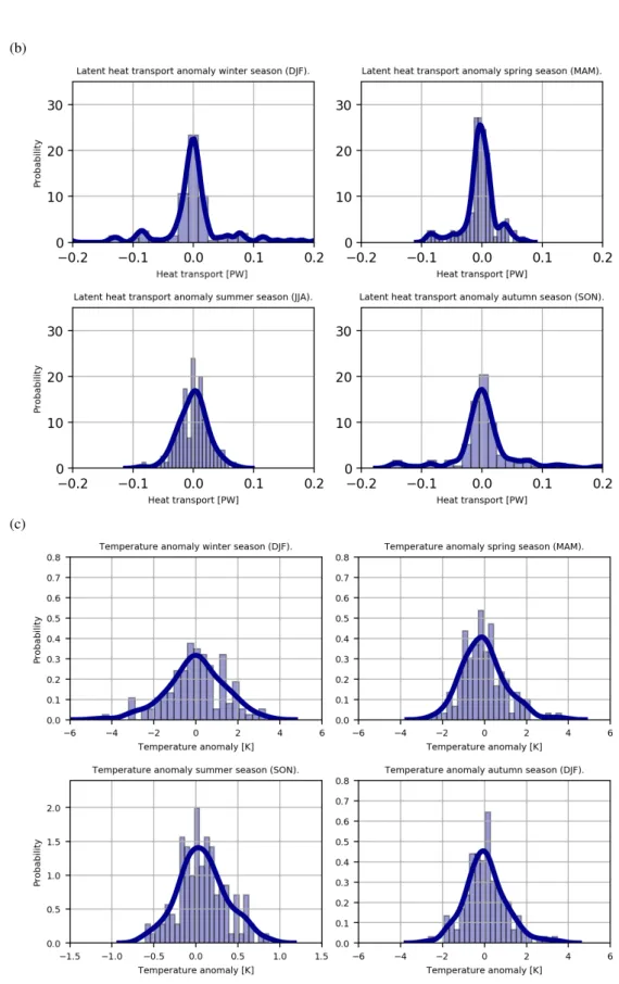
Figure 3.2 presents the seasonal distribution of the zonal monthly mean poleward heat transport anomalies at 70 N of H^? andH_L^? as well as the temperature anomalies of the polar cap poleward of 70 N. For both the heat transport anomalies as well as for the temperature anomalies we observe a much narrower distribution during the JJA season. In contrast, the winter period considering the months December, January and February (DJF) shows the largest variation in both temperature and heat transport. The main reason for weaker temperature anomalies during summer is the fact that the phase change from ice to liquid water does need a lot of energy. This means that during the melting season the incoming energy is partially used to melt ice. Additionally, during the summer season almost the entire polar cap northward of 70 N is constantly illuminated by the sun. While during wintertime heat transport is the main energy source of the Arctic, during summertime solar radiation also has a strong influence.

The observed pattern can be explained by the fact that during summertime the baroclinicity on the northern hemisphere is much weaker than during winter which results in weaker anomalies in the heat transport. When comparing the distribution of the heat transport anomalies with the temperature anomalies we find that both distributions show a very similar pattern. Motivated by the matching of both distributions we continue with a more detailed analysis by studying the correlation between heat transport anomalies into the Arctic and temperature anomalies in the Arctic.

(22)

Chapter 3 – Results

Figure 3.1: Histograms of zonal monthly mean poleward heat transport anomalies at 70 N and field mean of the temperature anomaly considering the polar cap poleward of 70 N.

(a)

(23)

(b)

(c)

Figure 3.2: Seasonal ordered histograms of (a) monthly mean H^?anomalies and (b)H^?_L anomalies at 70 N as well as (c) temperature anomalies considering the polar cap poleward of 70 N.

(24)

3.2 Correlation between heat transport and temperature anomalies

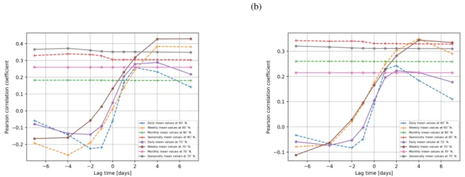
In this section, we analyse the correlation between heat transport and temperature anomalies in the Arctic region. Figure 3.3 shows the Pearson correlation between heat transportH^?anomalies at 70 N (resp. 80 N) and field mean temperature anomalies considering the polar cap poleward of 70 N (resp. 80 N) as a function of lag time. A lag time ofXdays means that we determine the Pearson correlation between the signal in the heat transport anomaly at the current day and the signal in the temperature anomaly with a delay ofXdays with respect to the heat transport. For bothH^?_L as well asH^? the Pearson correlation shows a symmetric distribution around 0 days lag time. The highest correlations are found using a lag time of 2 days for daily mean values and a lag time of 4 days for a weekly time range. When considering time ranges longer than a week the correlations do not vary significantly as a function of lag time.

(a) (b)

Figure 3.3: Correlation between (a) H^? anomalies and temperature anomalies and (b) H^?_L anomalies and temperature anomalies as a function of lag time for daily, weekly, monthly and seasonal time ranges. Dashed lines represent the polar cap poleward of 70 N and solid lines the polar cap northward of 80 N.

Based on the finding that the weekly time range with a lag time of 4 days results in the highest Pearson correlation values, we computed the same correlation as a function of the current month (Fig. 3.4). Analysing Fig. 3.4 we want to emphasise the following characteristics:

1. Pronounced seasonal cycle: H^?_L anomalies as well as theH^?anomalies show a pronounced seasonal variation.

Especially, when considering H_L^? anomalies we observe a strong yearly variation with peak correlation values between 0.5 - 0.6 during November to April and negative or very small correlations during the summer months June, July and August. Only the rise in the total heat transport correlation values between April to May interrupts this seasonal pattern.

2. Similar correlations for 70 N and 80 N:Both regions show very similar values and temporal patterns. The main difference is that the polar cap poleward of 80 N shows slightly higher correlation values during September to May.

3. Stable correlations for H_L^?during November to March: The latent heat transport anomalies show only little variation during the period between November to March.

4. Strong decrease in correlations from May to June: From May to June we observe a decrease in the correlations of more than 0.3.

One explanation for the points (1) and (4) is the start of the melting season in May. Additionally, the increased day length during summer also affects these correlations. A strong latent heat transport which brings moist and warm air into the Arctic can cause the formation of clouds which further affect the incoming solar radiation and the temperature of the polar cap. These highly dynamic feedback processes are difficult to characterize by the calculation of one-dimensional correlation values. We will therefore use a different approach to describe the effects of a strong latent heat transport anomaly on Arctic weather. In the following section, we analyse composites of the 10% most positive as well as the 10% most negative dailyH^?_Lanomalies at 70 N and describe its effects on temperature, cloud fraction, precipitation and thermal radiation.

(25)

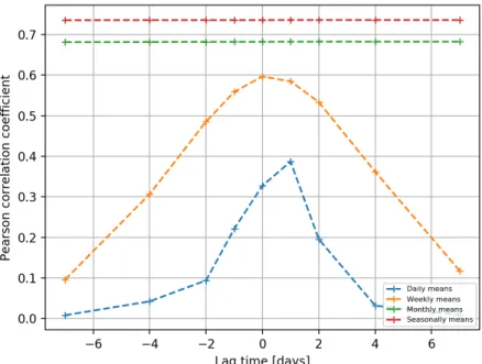
Figure 3.4: Pearson correlation betweenH^?_Lanomalies and temperature anomalies for a 7-day time range as a function of the current month considering the polar caps poleward of 70 N and 80 N. Between theH^?_Lanomalies and the temperature anomalies a lag time of 4 days was used.

3.3 Composites of synoptic situation based on anomalous H

^?_L

transport

In this section, we analyse anomalous H_L^?transport into the Arctic region. During the analysis we distinguish between extreme events with a pronounced positive and negativeH^?_Lanomaly. An extreme positive event is defined by an anomalous daily meanH^?_Ltransport at 70 N with a transport which exceeds the 90^thpercentile and an extreme negative event is related to aH^?_Lanomaly which is below the 10^thpercentile (Sec 2.4.2). In a series of consecutive heat transport events always the first day was chosen and the next event was considered only, if at least five days were in between the last day of the series and the following event. In Sec. 3.2, we show that there is a pronounced seasonal cycle in the Pearson correlation between heat transport and temperature anomalies. We therefore distinguish between the NDJFM and JJA time periods. During the NDJFM season correlation values are very stable with values close to 0.5. Whereas during the JJA season correlation values are below 0.2.

One particular challenge is that a strong latent heat transport anomaly does not lead to an instantaneous weather signal. In Fig. 3.5, we show that correlation between latent heat transport and temperature anomalies is delayed by around 4 days for weekly time ranges and by approximately 2 days when considering daily time scales. In order to account for the lag between the signal in the latent heat transport and its effect on other variables we consider 5-day mean values when analysing the anomalies of the following variables:

• Vertically integrated water vapor (VIWV)

• Temperature measured two meters above surface (T2M)

• Surface energy balance (SEB)

• Total cloud cover (TCC)

• Precipitation (PREC)

• Total column cloud liquid water (TCLW)

• Total column cloud ice water (TCIW).

(26)

For the additional variables:

• Poleward VIWV transport

• Cyclone frequency

• Surface freshwater flux (SFWF)

• Blocking frequency 1 pvu and 1.3 pvu: Blocks which are characterized by a vertical mean PV anomaly which is lower than - 1.0 pvu and - 1.3 pvu, respectively,

we analysed daily mean values.

3.3.1 Composites NDJFM season

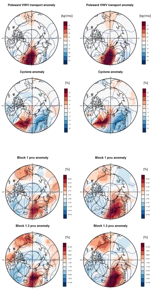
In this section, we analyse composites of anomalousH^?_Ltransport during the NDJFM period. Figure 3.5 shows composites based on events with extremeH_L^?anomalies at 70 N during the NDJFM period (see Sec. A.2.1 for events with extreme H_L^?anomalies at 80 N). The left column contains composites based on extreme positive moisture transport (H^?_Lanomalies above 90^thpercentile) and the right column composites based on extreme negative moisture transport (H^?_Lanomalies below the 10^thpercentile).

First, we focus on the VIWV transport anomalies. We observe that positive and negative anomalies show a similar regional pattern with peak anomalies in the Atlantic close to the prime meridian and smaller anomalies in the Pacific.

However, negative anomalies of VIWV transport do not show a pronounced peak and also range over a larger area reaching from Greenland’s east coast up to the Barents Sea. In addition, there is a difference by more than a factor of three in the magnitude of the VIWV transport anomalies with peak anomalies of up to 108_ms^kg compared to - 30^kg_ms. Analysing the 5-day mean VIWV anomalies we find peak values close to the regions with the strongest VIWV transport anomalies as well as in the Barents Sea. This finding indicates that a major part of the moisture transport in the Atlantic accumulates in the Barents Sea.

Focussing on T2M anomalies in Fig. 3.5, we observe that during extreme positive H^?_L events the strongest temperature anomalies are found close to Svalbard between the Greenland and Barents Seas. In this region, temperature anomalies exceed 1.125 K and reach peak values in Svalbard larger than 3.375 K. Additionally, there are also relatively low positive anomalies between 0.375 - 1.125 K present in the Bering Strait. In contrast, there are slightly negative temperature anomalies present in the Baffin Bay. Again, the corresponding negative anomalies of VIWV transport lead to a very similar pattern in T2M with negative anomalies between - 1.125 K up to - 2.625 K in the Barents Sea and slight positive anomalies in the Baffin Bay and over Southern Greenland. The SEB describing the exchange of energy between the surface and the atmosphere (Van den Broeke et al., 2011) reaches peak values in the Barents Sea and has a very similar regional distribution as the temperature anomalies.

Studying composites of blocking and cyclone frequency anomalies we observe that the strongest blocking frequency anomalies are found over Scandinavia. Positive anomalous H_L^?transport are related with an increased occurrence of positive blocking frequency anomalies over the Norwegian Sea. Considering that 1 pvu blockings occur over Scandinavia with a probability of around 5 - 10% during the NDJFM season, an anomaly of 18% means that blockings are almost four times more likely to occur during a strongH^?_Linto the Arctic.

Peak cyclone frequency anomalies are found east of Greenland with values of up to 27%. Since cyclones occur with a probability of around 15 - 25% during the NDFJM period over eastern Greenland, positiveH_L^?anomalies increase the likelihood of cyclones east of Greenland by a factor of 2 - 3. Contrary negativeH^?_Lanomalies almost lead to a reversed cyclone frequency anomaly pattern with approximately half the magnitude.

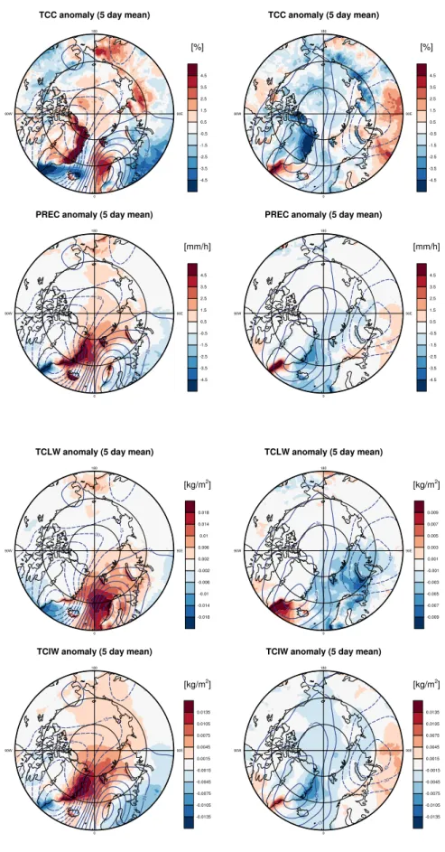
TCC and PREC show peak residual values at Greenland’s northeastern coast, Svalbard and west of Scandinavia as well as over northeastern Siberia. TCIW also shows peak values at Greenland’s east coast whereas the maxima of TCLW coincide with peak poleward VIWV transport anomalies.

(27)

(28)

Block 1 pvu anomaly Block 1 pvu anomaly

Block 1.3 pvu anomaly Block 1.3 pvu anomaly

(29)

Figure 3.5: Composites based on 10% most positive and negative poleward zonal daily mean H_L^?anomalies at 70 N considering the NDJFM season. Blue contours show geopotential anomalies at 500 hPa of the corresponding strongest

th

(30)

3.3.2 Composites JJA season

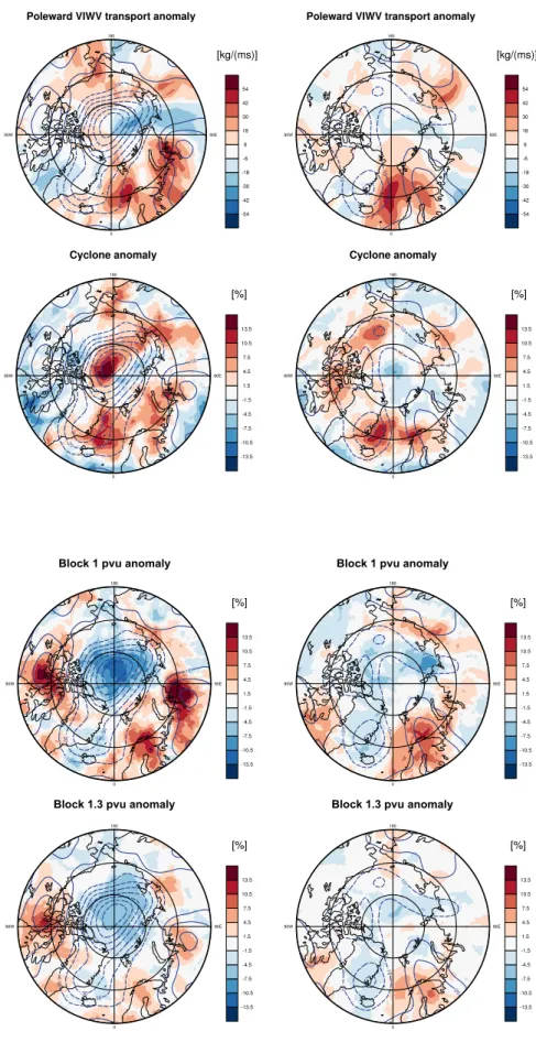
Additionally, we also investigate transport anomalies during the JJA season. In the summer period, where correlation coefficients between temperature andH_L^?anomalies are very low (< 0.2), the polar cap poleward 70 N is almost completely illuminated by the sun during the entire day (Liou, 1980). Figure 3.6 shows composites based on events with extremeH_L^? anomalies at 70 N during the JJA period (see A.2.2 for events with extremeH^?_Lanomalies at 80 N).

In contrast to the NDFJM period where VIWV transport anomalies are strongest over the ocean, in particular in the Atlantic, during summertime we observe peak moisture transport anomalies over land, especially over Siberia. Compared to the NDJFM period, the peak poleward VIWV transport anomalies are approximately four times smaller. Further- more, there is not a specific region with a particularly strong VIWV anomaly. However, strongH^?_L anomalies lead to an increase in the VIWV anomalies between 70 - 80 N, but do not cause a significant increase in VIWV northward of 80 N.

Considering T2M and SEB we find that positive VIWV transport anomalies do neither lead to a significant signal in the T2M anomaly nor in the SEB anomaly. Yet, a strong pattern is found when focussing on cyclone and blocking frequency anomalies. Strong positive H^?_L anomalies lead to a decrease in the 1 pvu blocking frequency anomaly of approximately 6% in the High Arctic. We further notice that cyclone frequency anomalies are located just slightly to the west of peak poleward VIWV transport anomalies. For positiveH^?_L anomalies TCC shows a pronounced peak over northern Greenland and in general values over the continent tend to have positive TCC anomalies whereas over the ocean TCC anomalies are small and mostly negative. StrongH^?_L anomalies lead to a significant increase in PREC anomalies over the entire polar cap poleward of 70 N. The regional distributions of PREC and TCIW are very similar. Additionally, the distribution of TCLW anomalies does match closely with the pattern of the TCC anomalies. Further notice that for most variables a negative moisture transport anomaly almost leads to a reversed pattern in comparison with cases which are linked with a positive moisture transport anomaly.

As a next step we investigate in more detail the regional distribution of the zonal poleward VIWV transport anomalies. The composites did reveal that during the NDJFM period strongest poleward VIWV transport are found in the Atlantic. During JJA, VIWV anomaly transport is found between approximately 0 - 180 E starting from the Farm Strait over whole northern Siberia up to the Bering Strait with a wave number of roughly 8. However, the composites come with the caveat that they do not provide any information about the relation between the probability of appearance and the strength of the signal. For instance, if there are days with a strong VIWV transport anomaly over the Bering Strait but their probability of appearance is much smaller compared to days with a similarly strong VIWV transport anomaly over the Atlantic, the composites will only show a weak anomaly over the Bering Strait. In Sec. 3.4, we account for this fact and analyse the regional distribution of poleward VIWV transport anomalies for each event separately.

(31)

(32)

Block 1 pvu anomaly Block 1 pvu anomaly

Block 1.3 pvu anomaly Block 1.3 pvu anomaly

(33)

Figure 3.6: Composites based on the 10% most positive and negative poleward zonal daily meanH_L^?anomalies at 70 N considering the JJA season. Blue contours show the geopotential anomalies at 500 hPa of the corresponding strongest

th