Impact of model resolution on Arctic sea ice and North Atlantic Ocean heat transport

(1)

https://doi.org/10.1007/s00382-019-04840-y

Impact of model resolution on Arctic sea ice and North Atlantic Ocean heat transport

David Docquier¹ · Jeremy P. Grist² · Malcolm J. Roberts³ · Christopher D. Roberts^3,4 · Tido Semmler⁵ · Leandro Ponsoni¹ · François Massonnet¹ · Dmitry Sidorenko⁵ · Dmitry V. Sein^5,6 · Doroteaciro Iovino⁷ · Alessio Bellucci⁷ · Thierry Fichefet¹

Received: 29 October 2018 / Accepted: 30 May 2019

Abstract

Arctic sea-ice area and volume have substantially decreased since the beginning of the satellite era. Concurrently, the poleward heat transport from the North Atlantic Ocean into the Arctic has increased, partly contributing to the loss of sea ice.

Increasing the horizontal resolution of general circulation models (GCMs) improves their ability to represent the complex interplay of processes at high latitudes. Here, we investigate the impact of model resolution on Arctic sea ice and Atlantic Ocean heat transport (OHT) by using five different state-of-the-art coupled GCMs (12 model configurations in total) that include dynamic representations of the ocean, atmosphere and sea ice. The models participate in the High Resolution Model Intercomparison Project (HighResMIP) of the sixth phase of the Coupled Model Intercomparison Project (CMIP6). Model results over the period 1950–2014 are compared to different observational datasets. In the models studied, a finer ocean resolution drives lower Arctic sea-ice area and volume and generally enhances Atlantic OHT. The representation of ocean surface characteristics, such as sea-surface temperature (SST) and velocity, is greatly improved by using a finer ocean resolution. This study highlights a clear anticorrelation at interannual time scales between Arctic sea ice (area and volume) and Atlantic OHT north of 60^◦N in the models studied. However, the strength of this relationship is not systematically impacted by model resolution. The higher the latitude to compute OHT, the stronger the relationship between sea-ice area/volume and OHT. Sea ice in the Barents/Kara and Greenland–Iceland–Norwegian (GIN) Seas is more strongly connected to Atlantic OHT than other Arctic seas.

Keywords Model resolution · Arctic sea ice · Ocean heat transport

1 Introduction

The recent accelerated loss of Arctic sea ice is undeniable, with declines in ice area and thickness during all months of the year and a progressive transition from multi-year to first-year ice (Vaughan et al. 2013; Notz and Stroeve 2016;

Barber et al. 2017; Petty et al. 2018). The annual mean Arctic sea-ice area has decreased by ∼2 million km² from 1979 to 2016 (Onarheim et al. 2018), i.e. an average loss of

∼53000 km²a⁻¹ , but sea-ice area displays strong regional and seasonal expressions. The perennial ice-covered seas (i.e. East Siberian, Chukchi, Beaufort, Laptev, and Kara) constitute the largest contributors to sea-ice loss in summer, while sea-ice loss in winter is dominated by the seasonally ice-covered seas located farther south (i.e. Barents, Okhotsk, Greenland, and Baffin), which are almost entirely ice-free in summer (Onarheim et al. 2018). Despite the uncertainty

* David Docquier

david.docquier@uclouvain.be

1 Earth and Life Institute, Université catholique de Louvain, Louvain-la-Neuve, Belgium

2 National Oceanography Centre, University of Southampton, Southampton, UK

3 Met Office Hadley Centre, Exeter, UK

4 European Centre for Medium Range Weather Forecasts, Shinfield Park, Reading, UK

5 Alfred Wegener Institute, Helmholtz Centre for Polar and Marine Research, Bremerhaven, Germany

6 Shirshov Institute of Oceanology, Russian Academy of Science, Moscow, Russia

7 Fondazione Centro Euro-Mediterraneo sui Cambiamenti Climatici (CMCC), Bologna, Italy

(2)

among the different thickness observational datasets (Zyg- muntowska et al. 2014), sea ice in the Central Arctic has significantly thinned since 1975 (Lindsay and Schweiger 2015; Kwok 2018).

Multiple mechanisms have contributed to the recent loss of Arctic sea ice, including anthropogenic global warming (Notz et al. 2016), changes in large-scale atmospheric circulation (Döscher et al. 2014) and ocean heat transport (OHT, Carmack et al. 2015), combined with powerful climate feed- backs acting in the Arctic (Goosse et al. 2018; Massonnet et al. 2018). A number of studies show that Arctic sea ice in the Atlantic sector (Barents, Kara, and Laptev Seas) is strongly influenced by Atlantic OHT (e.g. Sando et al. 2010;

Arthun et al. 2012; Ivanov et al. 2012; Polyakov et al. 2017).

Arthun et al. (2012) suggest that the recent observed sea- ice reduction in the Barents Sea occurred concurrently with an increase in Atlantic OHT due to both strengthening and warming of the oceanic inflow. Ivanov et al. (2012) also identify such a link between increased OHT and reduced Arctic sea ice in the western Nansen Basin, located north of Barents Sea, between Svalbard and Severnaya Zemlya.

They show that the location of specific zones with thinner ice and lower ice concentration mirrors the pathway of the Fram Strait branch of the Atlantic Water. Polyakov et al.

(2017) provide observational evidence that the ‘atlantifica- tion’ is also responsible for sea-ice loss in the eastern Eura- sian Basin. They argue that the recent increased penetration of Atlantic Water into the eastern Eurasian Basin, associated with stratification weakening and pycnocline warming, has led to a greater upward Atlantic Water heat flux to the ocean surface and a consequent reduction of ice growth in winter.

From a modeling perspective, Mahlstein and Knutti (2011) show that coupled general circulation models (GCMs) from the Coupled Model Intercomparison Project phase 3 (CMIP3) with the strongest northward OHT have the smallest September Arctic sea-ice extent and thickness. They suggest that improving the representation of OHT in GCMs (e.g. by using finer resolution) would lead to a smaller inter- model spread in the projections of the Arctic climate system.

Koenigk and Brodeau (2014) confirm the leading role of OHT in the current Barents Sea ice reduction through bottom melt using the EC-Earth model. However, their results do not indicate a clear impact of OHT on the Central Arctic sea ice. Three CMIP5 model outputs show that the increased OHT at the Barents Sea Opening (BSO) results in ice area reduction in the Barents Sea, while the enhanced OHT at Fram Strait influences sea-ice area variability in the Central Arctic via bottom melting (Sando et al. 2014a). A CMIP5 multi-model analysis suggests that enhanced Atlantic OHT has played a leading role in the recent observed decline in winter Barents sea-ice area (Li et al. 2017). Burgard and Notz (2017) analyze changes in the energy budget of the Arctic Ocean coming from 26 CMIP5 models and find that

the Arctic warming between 1961 and 2099 is driven by the net atmospheric surface flux in 11 models and by the meridional ocean heat flux in 11 models. This study shows a significant negative correlation between the Atlantic meridional ocean heat flux and Arctic sea-ice area across the models. The links between OHT and Arctic sea ice are further confirmed by a study using 40 Community Earth System Model Large Ensemble (CESM-LE) members (Auclair and Tremblay 2018), in which 80% of the rapid ice declines are correlated to increased OHT (mainly at the BSO and Bering Strait). The CESM-LE members further show that OHT in the Barents Sea is a major source of internal Arctic winter sea-ice variability and predictability (Arthun et al. 2019) and that the local contribution of internal variability strongly depends on the month and Arctic region analyzed (England et al. 2019).

The impact of model resolution on OHT has been analyzed in several studies. Roberts et al. (2016) run the HadGEM3-GC2 model with two different configurations (60 km in the atmosphere and 0.25^◦ in the ocean; 25 km in the atmosphere and 1∕12^◦ in the ocean) and show that a higher ocean resolution leads to stronger warm boundary currents, which results in higher sea-surface temperature (SST) and increased upward latent heat flux from the ocean to the atmosphere, thus providing a higher OHT. Similarly, Hewitt et al. (2016) and Roberts et al. (2018) find that poleward OHT increases with higher ocean resolution, but does not change significantly with finer atmosphere resolution, for their respective models (HadGEM3-GC2 and ECMWF-IFS, respectively). Grist et al. (2018) also find that a higher ocean resolution leads to higher Atlantic OHT in a multi-model comparison including three coupled GCMs with ocean resolutions ranging from 1^◦ to 1∕12^◦ . Other analyses reveal an improvement in OHT in the Barents Sea when GCMs are regionally downscaled to a resolution of ∼ 10 km (Sando et al. 2014b). The effect of resolution on Arctic sea ice has received less attention, but the study of Kirtman et al. (2012) shows that the use of a higher ocean resolution in the Com- munity Climate System Model version 3.5 (CCSM3.5), from 1.2^◦ to 0.1^◦ , results in ocean surface warming, especially in the Arctic and regions of strong ocean fronts. This warming is associated with a reduction of Arctic sea ice. The impact of model resolution on the relationships between Arctic sea ice and Atlantic OHT has not been investigated in detail yet.

Here, we provide the first detailed analysis of the horizontal resolution effect on Arctic sea ice, Atlantic OHT and relationships between both quantities. To this end, we use the outputs of five coupled GCMs (12 model configurations in total) that follow the protocol of the High Resolution Model Intercomparison Project (HighResMIP; Haarsma et al. 2016) and participate in the EU Horizon 2020 PRI- MAVERA project (PRocess-based climate sIMulation:

AdVances in high-resolution modelling and European

(3)

climate Risk Assessment, https ://www.prima vera-h2020 .eu/). It is important to note that only two model configurations in this study benefit from several member runs, which limits the assessment of internal variability. The goal of the present study is to quantify the impact of model resolution on Arctic sea-ice area and volume, then on North Atlantic OHT, and finally on the links between both Arctic sea ice and Atlantic OHT. Section 2 presents the model outputs and reference products (observations and reanalyses) used in this study. Section 3 provides our results in terms of Arctic sea ice, North Atlantic OHT and links between the two. Sec- tion 4 discusses the impact of model resolution, the impact of OHT on Arctic sea ice and some issues inherent to a multi-model analysis on resolution dependence. Finally, our conclusions are presented in Sect. 5.

2 Methodology

2.1 Models

Model outputs come from HighResMIP (Haarsma et al.

2016), which is one of the CMIP6-endorsed Model Inter- comparison Projects (MIPs). HighResMIP is the first climate multi-model approach dedicated to the systematic investi- gation of the role of horizontal resolution. We mainly use the model outputs of coupled historical runs (referred to as

‘hist-1950’ in HighResMIP), in order to compare our results to observations. We also analyze the outputs of coupled control runs (‘control-1950’ in HighResMIP, using a constant atmospheric forcing corresponding to the year 1950) and compare them to historical runs. This allows one to check whether the results obtained depend on the forcing or not.

Both hist-1950 and control-1950 runs start in 1950 at the end of a 30–50-year spin-up and are integrated for 65 years (until 2014). Five different GCMs (12 model configurations in total), representing the atmosphere, ocean and sea ice, are considered in this study. Each model has a ‘low’

and a ‘high’ (or ‘medium’) resolution configuration, and two of these models also have an ‘intermediate’ resolution configuration. In the following text, when we use the word

‘resolution’ without specifying whether it is atmosphere or ocean resolution, we mean atmosphere and ocean resolutions combined. Our study is limited by the number of ensemble members available: only two model configurations have different members (see text below). Thus, a clear assessment of internal variability is not possible in the context of this analysis. A summary of model characteristics is given in Table 1.

The first model is the Global Coupled 3.1 configuration of the Hadley Centre Global Environmental Model 3 (HadGEM3-GC3.1; Williams et al. 2018), hereafter referred to as HadGEM3. It is formed by the Global Atmosphere

7.1 (GA7.1), Global Land 7.0 (GL7.0), Global Ocean 6.0 (GO6.0, Storkey et al. 2018) and Global Sea Ice 8.1 (GSI8.1) components. The atmosphere and land components are based on the Unified Model (UM; Cullen 1993) and Joint UK Land Environment Simulator (JULES; Best et al.

2011), respectively. The ocean component is version 3.6 of the Nucleus for European Modelling of the Ocean (NEMO, Madec 2016), consisting of a hydrostatic, finite-difference, primitive-equation general circulation model. It is coupled to version 5.1 of the Los Alamos sea-ice model (CICE; Hunke et al. 2015). We use three different HadGEM3 configurations having different horizontal resolutions. The first configuration, HadGEM3-LL, uses the N96 atmosphere grid (nominal resolution of 250 km, i.e. 135 km at 50^◦N ) and ORCA1 tripolar ocean grid (resolution of 1^◦ ). The second configuration, HadGEM3-MM, runs with the N216 atmosphere grid (nominal resolution of 100 km, i.e. 60 km at 50^◦N ) and ORCA025 ocean grid (resolution of 0.25^◦ ). The third configuration, HadGEM3-HM, uses the N512 atmosphere grid (nominal resolution of 50 km, i.e. 25 km at 50^◦N ) and the same ocean resolution as HadGEM3-MM ( 0.25^◦ ). A few parameters change between the three configurations, but stay limited to resolution-dependent parameterizations (Table 1).

One of the main differences is the albedo of snow on sea ice, which is smaller by 2% in HadGEM3-LL compared to HadGEM3-MM and HadGEM3-HM due to overestimation of Arctic sea-ice area and volume at low resolution compared to observations (Kuhlbrodt et al. 2018).

The second model is the European Centre for Medium- Range Weather Forecasts Integrated Forecast System (ECMWF-IFS) cycle 43r1 (Roberts et al. 2018). The atmospheric component of the ECMWF-IFS model is a hydrostatic, semi-Lagrangian, semi-implicit dynamical-core model using a cubic octahedral reduced Gaussian (Tco) grid. The land surface component is the Hydrology Tiled ECMWF Scheme of Surface Exchanges over Land (HTES- SEL; Balsamo et al. 2009). The ocean and sea ice components are based on version 3.4 of NEMO and version 2 of the Louvain-la-Neuve Sea-Ice Model (LIM2; Fichefet and Morales Maqueda 1997), respectively. In this study, we use three configurations of the ECMWF-IFS model run at different horizontal resolutions. The low-resolution configuration, referred to as ECMWF-LR, uses the Tco199 atmosphere grid (nominal resolution of 50 km) and ORCA1 ocean grid. The high-resolution configuration, named ECMWF-HR, uses the Tco399 atmosphere grid (nominal resolution of 25 km) and ORCA025 ocean grid. The intermediate-resolution configuration, ECMWF-MR, has the same atmosphere resolution as ECMWF-LR (Tco199) and the same ocean resolution as ECMWF-HR (ORCA025). All three configurations are configured to be as close as possible to each other with differences limited to resolution-dependent parameterizations (Table 1). Six members are available for ECMWF-LR and

(4)

Table 1 Characteristics of the models used in this study. n/a: not applicable

HadGEM3 ECMWF-IFS AWI-CM CMCC-CM2 MPI-ESM

Configurations LL: ‘low’ resolution LR: ‘low’ resolution LR: ‘low’ resolution HR4: ‘low’ resolution HR: ‘low’ resolution MM: ‘medium’ reso-

lution

HM: ‘high’ resolution in atm.; ‘medium’

resolution in ocean

MR: ‘low’ resolution in atm.; ‘high’ resolution in ocean HR: ‘high’ resolution

HR: ‘high’ resolution VHR4: ‘high’ resolu-

tion XR: ‘high’ resolution

Atmosphere

Model UM IFS cycle 43r1 ECHAM6.3 CAM4 ECHAM6.3

Grid type Grid point Spectral Spectral Grid point Spectral

Grid name LL: N96 LR/MR: Tco199 LR: T63 HR4: 1^◦ HR: T127

MM: N216 HR: Tco399 HR: T127 VHR4: 0.25◦ XR: T255

HM: N512 Nominal resolution

(km) LL: 250 LR/MR: 50 LR: 250 HR4: 100 HR: 100

MM: 100 HR: 25 HR: 100 VHR4: 25 XR: 50

HM: 50

Resolution 50^◦N (km) LL: 135 LR/MR: 50 LR: 129 HR4: 64 HR: 67

MM: 60 HR: 25 HR: 67 VHR4: 18 XR: 34

HM: 25

Vertical levels 85 91 LR: 47 26 95

HR: 95

Time step (min) LL: 20 LR/MR: 30 LR: 6.7 30 HR: 3.3

MM: 15 HR: 20 HR: 3.3 XR: 1.5

HM: 10 Ocean—sea ice

Ocean/sea-ice model NEMO3.6/CICE5.1 NEMO3.4/LIM2 FESOM NEMO3.6/CICE4.0 MPIOM1.6.3

Grid type Curvilinear Curvilinear Unstructured Curvilinear Curvilinear

Numerical method Finite difference Finite difference Finite element Finite difference Finite difference

Grid name LL: ORCA1 LR: ORCA1 FESOM ORCA025 TP04

MM/HM: ORCA025 MR/HR: ORCA025

Resolution LL: 1^◦ LR: 1^◦ LR: 24-110 km 0.25^◦ 0.4^◦

MM/HM: 0.25^◦ MR/HR: 0.25^◦ HR: 10-60 km

Vertical levels 75 75 46 50 40

Time step (min) LL: 30 LR: 60 LR: 15 20 60

MM/HM: 20 MR/HR: 20 HR: 10

Gent and McWilliams (1990) eddy param- eterization

LL: yes LR: yes Gradually switched

off between 50 and 25 km

No Yes

MM/HM: no MR/HR: no

Horizontal momentum

diffusion LL: 2×10⁴m²s⁻¹ LR:10⁴m²s⁻¹ Varying −1.8×10¹¹m⁴s⁻¹ Varying MM/HM:

−1.5×10¹¹m⁴s⁻¹

MR/HR:

−1.1×10¹¹m⁴s⁻¹ Background verti-

cal eddy viscosity ( m²s⁻¹)

1.2×10⁻⁴ LR: 1.2×10⁻⁴ 10⁻⁴ 1.2×10⁻⁴ 5×10⁻⁵

MR/HR: 1.0×10⁻⁴ Background verti-

cal eddy diffusivity ( m²s⁻¹)

1.2×10⁻⁵ LR: 1.2×10⁻⁵ 10⁻⁵−10⁻⁴ 1.2×10⁻⁵ 1.05×10⁻⁵ MR/HR: 1.0×10⁻⁵

Isopycnal tracer dif-

fusivity ( m²s⁻¹) LL: 1000 LR: 1000 1500 at 1◦ , scaled with

resolution 300 250

MM/HM: 150 MR/HR: 300

Eddy-induced velocity coefficient ( m²s⁻¹)

LL: 1000 LR: 1000 Varying n/a 250

MM/HM: n/a MR/HR: n/a

(5)

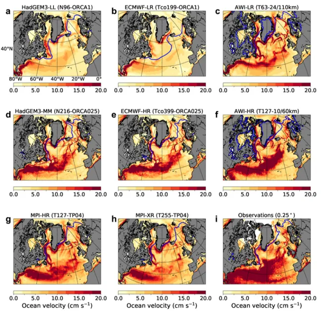
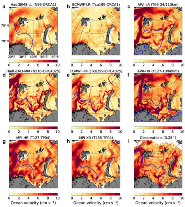
four members for ECMWF-HR (see Roberts et al. 2018 for further details). In the present study, we present the results of the ensemble means of both ECMWF-LR and ECMWF-HR, except in Figs. 7, 8, 9 and 10, where we show results from the first member of these configurations.

The third model is version 1.1 of the Alfred Wegener Institute Climate Model (AWI-CM; Sidorenko et al. 2015;

Rackow et al. 2018). It is made up of version 6.3 of the Euro- pean Centre/Hamburg (ECHAM6.3) atmospheric model and version 1.4 of the Finite Element Sea ice-Ocean Model (FESOM; Wang et al. 2014; Sein et al. 2016). ECHAM is a spectral model and includes the land surface model JSBACH (Stevens et al. 2013). The FESOM ocean-sea ice component employs an unstructured mesh, which allows using enhanced horizontal resolution in dynamically active regions while keeping a coarse-resolution setup otherwise. Two model configurations of AWI-CM at different horizontal resolutions are used in the present study. The first configuration, AWI-LR, uses the T63 atmosphere grid (nominal resolution of 250 km, i.e. 129 km at 50^◦N ) and an ocean mesh with resolution varying from 24 km to 110 km ( ∼90 km in the vicinity of the Gulf Stream and ∼25 km in the Arctic). The second configuration, AWI-HR, uses the T127 atmosphere grid (nominal resolution of 100 km, i.e. 67 km at 50^◦N ) and an ocean mesh varying from 10 to 60 km, with a refined resolution in key ocean straits ( ∼10 km in the vicinity of the Gulf Stream and ∼25 km in the Arctic). Details on the two ocean meshes are in Sein et al. (2016). Beside the resolution, small differences (e.g. model time step) exist between both configurations and are noted in Table 1.

The fourth model is version 2 of the Euro-Mediterranean Centre on Climate Change Climate Model (CMCC-CM2;

Cherchi et al. 2018). It is composed of version 4 of the Community Atmosphere Model (CAM; Neale et al. 2013), NEMO3.6 for the ocean, CICE4.0 for sea ice, and version 4.5 of the Community Land Model (CLM, Oleson et al.

2013). Two configurations of CMCC-CM2 are employed in this analysis. They both make use of the same ocean resolution (ORCA025, i.e. 0.25^◦ ). The first configuration, CMCC- HR4, has a resolution of 1^◦ in the atmosphere (64 km at

50^◦N ), while the second configuration, CMCC-VHR4, has a resolution of 0.25^◦ (18 km at 50^◦N ). No other difference exists between the two configurations.

The fifth model is version 1.2 of the Max Planck Institute Earth System Model (MPI-ESM, Müller et al. 2018). The ECHAM6.3 atmospheric component is coupled to version 1.6.3 of the Max Planck Institute Ocean Model (MPIOM, Jungclaus et al. 2013). MPIOM is a free-surface ocean-sea ice model that solves the primitive equations with the hydrostatic and Boussinesq approximations. The two model configurations of MPI-ESM used in this study employ the same ocean model grid, i.e. the 0.4^◦ tripolar grid (TP04). They differ by their atmosphere resolution: the low-resolution configuration, MPI-HR, uses the T127 grid (nominal resolution of 100 km, i.e. 67 km at 50^◦N ), while the high-resolution configuration, MPI-XR, runs on the T255 grid (nominal resolution of 50 km, i.e. 34 km at 50^◦N ). Beside the atmosphere horizontal resolution, the only difference between both configurations is the atmosphere model time step (Table 1).

For the five models used here, we retrieve monthly mean sea-ice concentration (‘siconc’ CMIP6 variable), equivalent sea-ice thickness (‘sivol’; i.e. mean sea-ice volume per grid- cell area), SST (‘tos’), zonal and meridional components of ocean velocity (‘uo’ and ‘vo’), ocean potential temperature (‘thetao’), Atlantic OHT, as well as grid-cell area. The OHT in HadGEM3, CMCC-CM2 and MPI-ESM simulations is computed online (‘hfbasin’ CMIP6 variable). For AWI-CM and ECMWF-IFS, OHT is not available as a model output, so it is computed offline. For AWI-CM, OHT is the sum of the heat transport computed from the total heat flux applied at the ocean surface (atmosphere/ocean exchanges) and the transport derived from the vertically integrated heat tenden- cies (ocean accumulation, release of heat). For ECMWF- IFS, OHT is computed from monthly mean products of meridional velocity and potential temperature of the ocean (which take the sub-monthly eddy variability into account).

All model outputs represent the total OHT as they include both the time-mean and transient (eddy) contributions.

It is important to note that we compute Arctic sea-ice area (and not sea-ice extent) in this study, due to uncertainties in

Table 1 (continued)

HadGEM3 ECMWF-IFS AWI-CM CMCC-CM2 MPI-ESM

Albedo of snow on

sea ice LL: 0.68 No change No change No change No change

MM/HM: 0.70

References Williams et al. (2018) Roberts et al. (2018) Sidorenko et al.

(2015) Cherchi et al. (2018) Müller et al. (2018) CMIP6 metadata LL: MOHC (2018b) LR: ECMWF (2018b) LR: AWI (2018b) HR4: CMCC (2018a) HR: MPI-M (2018)

MM: MOHC (2018c) MR: ECMWF (2018c) HR: AWI (2018a) VHR4: CMCC

(2018b) XR: MPI-M (2019)

HM: MOHC (2018a) HR: ECMWF (2018a)

(6)

modeled sea-ice extent arising from the grid geometry (Notz 2014). We retrieve this quantity from sea-ice concentration and area of model grid cells. Sea-ice volume is computed from equivalent sea-ice thickness (‘sivol’) and area of grid cells.

2.2 Reference products

Several observational and reanalysis datasets are used in the present analysis in order to evaluate model results.

For sea-ice concentration, the second version of the global sea-ice concentration climate data record (OSI-450) from the European Organisation for the Exploitation of Meteorological Satellites Ocean Sea Ice Satellite Applica- tion Facility (EUMETSAT OSI SAF 2017) is used (Lavergne et al. 2019). This dataset covers the period from 1979 to 2015 and is derived from passive microwave data from Scanning Multichannel Microwave Radiometer (SMMR), Special Sensor Microwave/Imager (SSM/I) and Special Sensor Microwave Imager Sounder (SSMIS). In our study, we use the data from 1979 to 2014 to be consistent with HighResMIP model outputs. The OSI SAF algorithm to retrieve sea-ice concentration from brightness temperature is a hybrid method combining an algorithm that is tuned to perform better over open-water and low-concentration conditions and an algorithm that is tuned to perform better over closed-ice and high-concentration conditions (Lavergne et al. 2019). The spatial resolution of this dataset is 25 km and its accuracy for sea-ice retrieval in the Northern Hemi- sphere is 5% (EUMETSAT OSI SAF 2017). We compute the monthly mean concentration from daily data.

For sea-ice thickness, we use the Ice, Cloud, and land Elevation Satellite (ICESat) gridded data at a spatial resolution of 25 km (Kwok et al. 2009). This satellite altimeter provides sea-ice freeboard height, from which sea-ice thickness is derived based on spatially varying snow depth (from the ECMWF snowfall accumulation fields) and densities of ice (constant), snow (seasonal behavior) and water (constant). The coverage period is limited to the months of Octo- ber–November and February–March from 2003 to 2008.

The mean absolute uncertainty of this dataset is 0.21 m in October–November and 0.28 m in February–March (Zyg- muntowska et al. 2014).

Monthly mean sea-ice thickness from the Pan-Arctic Ice- Ocean Modeling and Assimilation System (PIOMAS) is also considered for the period 1979–2014. PIOMAS is a coupled ocean and sea-ice model with capability of assimilating daily sea-ice concentration and SST. It is based on the Parallel Ocean Program (POP) coupled to a multi-category thickness and enthalpy distribution (TED) sea-ice model (Zhang and Rothrock 2003). The model is driven by daily National Centers for Environmental Prediction / National Center for Atmospheric Research (NCEP/NCAR) reanalysis surface

forcing fields. The mean horizontal resolution in the Arctic is 22 km. PIOMAS data agree well with ICESat ice thickness retrievals over the Central Arctic with a mean difference lower than 0.1 m (Schweiger et al. 2011). However, the trend in ice thickness varies by about 40-50% depending on the atmospheric forcing used to drive the model (Lindsay et al.

2014) and care needs to be taken when using this product (Chevallier et al. 2017).

For the poleward Atlantic OHT, we use annual mean estimates from Trenberth and Caron (2001) that cover the period from February 1985 to April 1989. These estimates are computed on a 2.8^◦ grid by combining top-of-the- atmosphere (TOA) radiation data from the Earth Radiation Budget Experiment (ERBE) with NCEP/NCAR reanalysis.

They show a relatively good agreement compared to direct measurements of Atlantic OHT. The more recent estimates from Trenberth and Fasullo (2017) are also used and cover the period 2000–2014 on a 1^◦ grid. They are based on TOA radiation data from Clouds and the Earth’s Radiant Energy System (CERES), ECMWF Interim Re-Analysis (ERA- Interim) and ocean heat content from Ocean ReAnalysis Pilot v5 (ORAP5) reanalysis. In addition, we use OHT estimates derived from the Rapid Climate Change-Meridi- onal Overturning Circulation and Heatflux Array (RAPID- MOCHA; Johns et al. 2011). The RAPID-MOCHA array is an observing system deployed at 26.5^◦N , near the latitude of maximum Atlantic OHT. This array allows to provide con- tinuous measurements from April 2004. We also use direct hydrographic measurements of Atlantic OHT coming from different expeditions ( 30^◦S , 11^◦S , 8^◦N , 14^◦N , 24^◦N , 57^◦N ) and reported in Fig. 1 of Grist et al. (2018). Finally, we use OHT estimates at the BSO (71.5–73.5^◦N , 20^◦E ) derived from hydrographic data and current meter moorings coming from the Institute of Marine Research (IMR, Norway).

These data were kindly provided by R. Ingvaldsen and span the period from 1997 to 2017.

For SST, we use version 2 of the National Oceanic and Atmospheric Administration (NOAA) Optimum Interpola- tion Sea Surface Temperature (OI SST) analysis. These data are provided at a spatial resolution of 0.25^◦ and a temporal resolution of one day, from September 1981 to present. In our study, we compute monthly mean SST from daily data and we use data from 1982 to 2014 to be consistent with model outputs. The OI SST analysis combines Advanced Very High Resolution Radiometer (AVHRR) satellite data and in-situ observations from ships and buoys on a regular global grid following the procedure described in Reynolds et al. (2007). Daytime and nighttime satellite observations are adjusted to the daily average of in-situ (ships and buoys) data. All satellite data are bias adjusted relative to seven days of in-situ data using a spatially smoothed 7-day in situ SST average.

(7)

We finally retrieve the ocean surface absolute geostrophic velocities (zonal and meridional components) provided by the Sea Level Thematic Assembly Centre (SL TAC) through the Copernicus Marine Environment Monitoring Service (CMEMS). We use the reprocessed gridded daily data provided at a spatial resolution of 0.25^◦ . In our study, we compute monthly means over the period 1993–2016. This is a multi-mission altimeter data processing system (Jason- 3, Sentinel-3A, HY-2A, Saral/AltiKa, Cryosat-2, Jason-2, Jason-1, T/P, ENVISAT, GFO, ERS1/2), where all mis- sions are homogenized with respect to the reference OSTM/

Jason-2 mission. These altimeter data are in relatively good agreement with in-situ observations of the North Atlantic Current (Roessler et al. 2015) and the Norwegian Atlantic Slope Current (Skagseth et al. 2004). Errors in geostrophic currents from this dataset range between 5 and 15 cm s⁻¹ depending on the ocean surface variability (Pujol 2017).

3 Results

3.1 Arctic sea ice

Figures 1 and 2 show monthly mean Arctic sea-ice area and volume, respectively, averaged over 1979–2014. This period is chosen to be comparable to observations, but key results are independent of the chosen period. For all of the

models used in this study, we find a year-round decrease of Arctic sea-ice area and volume with finer ocean resolution (comparing HadGEM3-LL with HadGEM3-MM/

HM, ECMWF-LR with ECMWF-MR/HR, and AWI-LR with AWI-HR). This decrease is especially pronounced for ECMWF-IFS, i.e. −23% to −30% in area (Table 2) and −36 to −49% in volume (Table 3) over the whole period. The change in sea-ice area and volume is less clear with chang- ing atmosphere resolution. For HadGEM3, increasing the atmosphere resolution from 100 (HadGEM3-MM) to 50 km (HadGEM3-HM) leads to lower sea-ice area and volume (Figs. 1, 2). However, sea-ice area and volume increase with finer atmosphere resolution for ECMWF-IFS (from 50 km in ECMWF-MR to 25 km in ECMWF-HR) and CMCC-CM2 (from 100 km in CMCC-HR4 to 25 km in CMCC-VHR4).

For MPI-ESM, sea-ice area generally increases with higher atmosphere resolution, although the increase is relatively small and not significant over the whole time period (Fig. 1, Table 2), while sea-ice volume decreases (Fig. 2, Table 3).

Thus, the implication from this sample of models is that a finer ocean resolution leads to reduced Arctic sea-ice area and volume, while the impact of atmosphere resolution is less clear. This point will be further discussed in Sect. 4.1.

Both HadGEM3 and ECMWF-IFS models generally overestimate sea-ice area and volume during all months compared to OSI SAF (Fig. 1) and PIOMAS (Fig. 2), respectively, with an unrealistically high volume for the

Fig. 1 Monthly mean Arctic sea-ice area averaged over 1979–2014 (1979–2013 for AWI-LR and AWI-HR). Results from HighResMIP hist-1950 model outputs and OSI SAF satellite observations. The black line on top of each bar indicates the temporal standard deviation

Fig. 2 Monthly mean Arctic sea-ice volume averaged over 1979–2014 (1979–2010 for AWI-LR and AWI-HR). Results from HighResMIP hist-1950 model outputs and PIOMAS reanalysis. The black line on top of each bar indicates the temporal standard deviation

(8)

ECMWF-LR configuration. For HadGEM3 and ECMWF- IFS, using a finer ocean resolution provides results in better agreement with both sea-ice area from OSI SAF (Fig. 1) and sea-ice volume from PIOMAS (Fig. 2). ECMWF-MR is very close to the observed sea-ice area, and HadGEM3-HM is in good agreement with the sea-ice volume from PIOMAS. The situation is not as clear-cut for AWI-CM, CMCC-CM2 and MPI-ESM models. Both AWI-CM configurations overestimate sea-ice area in winter and underestimate it in summer compared to observations. The finer resolution (AWI-HR) is closer to OSI SAF sea-ice area during December-May, and farther away the rest of the year compared to AWI-LR (Fig. 1). CMCC-HR4 underestimates sea-ice area, while CMCC-VHR4 stays within the bounds of interannual variability of OSI SAF (Fig. 1). MPI-ESM sea-ice area agrees with OSI SAF within the bounds of interannual variability in winter and underestimates this quantity in summer. The finer resolution of MPI-ESM (MPI-XR) is closer to OSI SAF in terms of sea-ice area from November to March and June, and farther away the rest of the year compared to MPI-HR (Fig. 1). Both AWI-CM and MPI-ESM slightly underestimate sea-ice volume compared to PIOMAS, with the coarser resolutions of these two models being closer to PIOMAS

during the whole year (Fig. 2). CMCC-HR4 slightly over- estimates the sea-ice volume from reanalysis, while CMCC- VHR4 clearly has too high ice volume (Fig. 2).

Despite these model biases, all five models can reproduce the general behavior of the mean seasonal cycles of Arctic sea-ice area and volume compared to OSI SAF observations (Fig. 1) and PIOMAS reanalysis (Fig. 2), respectively, with a maximum in March for area and April for volume, and a minimum in August-September for area and September for volume. All HadGEM3, AWI-CM and MPI-ESM configurations, as well as the low resolution of ECMWF-IFS, overestimate the amplitude of the mean seasonal cycles of Arctic sea-ice area and volume compared to OSI SAF observations (Fig. 1) and PIOMAS reanalysis (Fig. 2), respectively. The two higher resolutions of ECMWF-IFS and the two CMCC-CM2 configurations underestimate these cycles.

Using a finer resolution has different implications on the amplitude of the seasonal cycles of sea-ice area and volume for the different models. For HadGEM3, the amplitude decreases and is in better agreement with observations/

reanalysis at finer ocean resolution. For ECMWF-IFS, the amplitude also decreases with finer ocean resolution, but the coarser resolution (ECMWF-LR) has an amplitude of

Table 2 Mean differences in Arctic sea-ice area ( 10⁶km² ) between the different configurations of each model averaged over all months of the period 1979–2014, over winter months (January–March 1979–2014), and over summer months (July to September 1979–2014)

The relative differences (in % ) are given in brackets. Significant differences ( 5% level) are indicated in bold font. Italic is used when ocean resolution is different between configurations

Model differences All months January–March July–September

HadGEM3-MM - HadGEM3-LL −𝟏.𝟏𝟖(−𝟖%) −𝟐.𝟎𝟏(−𝟏𝟎%) − 0.20(−3%) HadGEM3-HM - HadGEM3-MM −𝟏.𝟒𝟎(−𝟏𝟏%) −𝟏.𝟖𝟎(−𝟏𝟎%) −𝟏.𝟎𝟒(−𝟏𝟒%) HadGEM3-HM - HadGEM3-LL −𝟐.𝟓𝟖(−𝟏𝟗%) −𝟑.𝟖𝟏(−𝟐𝟎%) −𝟏.𝟐𝟒(−𝟏𝟔%) ECMWF-HR - ECMWF-LR −𝟑.𝟑𝟗(−𝟐𝟑%) −𝟒.𝟑𝟐(−𝟐𝟒%) −𝟐.𝟕𝟖(−𝟐𝟔%) ECMWF-MR - ECMWF-LR −𝟒.𝟑𝟓(−𝟑𝟎%) −𝟓.𝟐𝟗(−𝟐𝟗%) −𝟑.𝟕𝟎(−𝟑𝟓%) ECMWF-HR - ECMWF-MR +𝟎.𝟗𝟔(+𝟗%) +𝟎.𝟗𝟕(+𝟕%) +𝟎.𝟗𝟐(+𝟏𝟑%) AWI-HR - AWI-LR −𝟏.𝟓𝟖(−𝟏𝟒%) −𝟏.𝟓𝟔(−𝟗%) −𝟏.𝟕𝟎(−𝟑𝟑%) CMCC-VHR4 - CMCC-HR4 +𝟏.𝟔𝟏(+𝟏𝟖%) +𝟏.𝟕𝟒(+𝟏𝟒%) +𝟏.𝟓𝟕(+𝟑𝟎%) MPI-XR - MPI-HR + 0.21 ( +2%) +𝟏.𝟎𝟓(+𝟖%) −𝟎.𝟗𝟓(−𝟐𝟎%)

Table 3 Mean differences in Arctic sea-ice volume ( 10³km³ ) between the different configurations of each model averaged over all months of the period 1979–2014, over winter months (January to March 1979–2014), and over summer months (July to September 1979–2014)

HadGEM3-MM - HadGEM3-LL −0.62(−2%) −𝟏.𝟐𝟔(−𝟒%) +0.31(+1%) HadGEM3-HM - HadGEM3-MM −𝟒.𝟐𝟎(−𝟏𝟓%) −𝟒.𝟏𝟐(−𝟏𝟑%) −𝟒.𝟐𝟗(−𝟐𝟎%) HadGEM3-HM - HadGEM3-LL −𝟒.𝟖𝟐(−𝟏𝟕%) −𝟓.𝟑𝟗(−𝟏𝟔%) −𝟑.𝟗𝟖(−𝟏𝟗%) ECMWF-HR - ECMWF-LR −𝟐𝟏.𝟏𝟕(−𝟑𝟔%) −𝟐𝟐.𝟓𝟒(−𝟑𝟓%) −𝟏𝟗.𝟕𝟎(−𝟑𝟖%) ECMWF-MR - ECMWF-LR −𝟐𝟖.𝟔𝟒(−𝟒𝟗%) −𝟑𝟎.𝟏𝟏(−𝟒𝟕%) −𝟐𝟔.𝟗𝟔(−𝟓𝟐%) ECMWF-HR - ECMWF-MR +𝟕.𝟒𝟕(+𝟐𝟓%) +𝟕.𝟓𝟕(+𝟐𝟐%) +𝟕.𝟐𝟔(+𝟑𝟎%) AWI-HR - AWI-LR −𝟒.𝟒𝟕(−𝟐𝟓%) −𝟒.𝟑𝟑(−𝟏𝟖%) −𝟒.𝟔𝟖(−𝟒𝟖%) CMCC-VHR4 - CMCC-HR4 +𝟏𝟓.𝟕𝟎(+𝟔𝟐%) +𝟏𝟔.𝟏𝟕(+𝟓𝟕%) +𝟏𝟓.𝟐𝟐(+𝟕𝟑%)

MPI-XR - MPI-HR −𝟑.𝟏𝟐(−𝟏𝟕%) −𝟐.𝟐𝟕(−𝟏𝟎%) −𝟒.𝟏𝟔(−𝟒𝟏%)

(9)

sea-ice area that is closer to observations, while the amplitude of sea-ice volume is closer to PIOMAS with the finer resolutions (ECMWF-MR/HR). For AWI-CM, the amplitude stays relatively similar between both ocean resolutions.

For CMCC-CM2, the amplitude slightly increases and is in better agreement with observations with finer atmosphere resolution. For MPI-ESM, the amplitude increases with finer atmosphere resolution, and the coarser resolution has an amplitude closer to observations.

In agreement with OSI SAF observations and PIOMAS reanalysis, the trends in Arctic sea-ice area and volume over 1979–2014 are significantly negative ( 5% level) for all models and all months (Figs. 3 and 4). Compared to observations and reanalysis, the trends in sea-ice area and volume of HadGEM3-LL, ECMWF-LR and MPI-HR are generally more negative than the observed and reanalysis trends. On the contrary, the trends in area and volume of HadGEM3-HM, ECMWF-MR, ECMWF-HR, AWI-LR and MPI-XR are generally less negative than the observed and reanalysis trends. The two CMCC-CM2 configurations have trends in sea-ice volume that are more negative than PIOMAS during the whole year, while they have trends in sea-ice area that are less negative than OSI SAF in summer. AWI-HR has a trend in sea-ice volume that is less negative than PIOMAS. For all models, the trends in sea-ice area and volume are less negative with finer ocean

resolution, with the exception of AWI-CM for which the trend in sea-ice area becomes more negative with finer resolution. As for mean values, the impact of atmosphere resolution on trends in area and volume is not clear, with less negative trends for HadGEM3 (comparing HadGEM3- MM and HadGEM3-HM) and MPI-ESM, and more negative trends for ECMWF-IFS (comparing ECMWF-MR and ECMWF-HR) and CMCC-CM2 (Figs. 3 and 4). The higher resolution configurations do not necessarily have sea-ice area and volume trends in closer agreement with observations and reanalysis. Comparing the mean sea-ice volume (Fig. 1) and the trend in sea-ice volume (Fig. 3), we find that models with lower mean sea-ice volume generally have less negative trends in sea-ice volume. This can be explained by the ice growth-thickness feedback, i.e.

models with thinner sea ice have larger ice-growth rates, partly limiting sea-ice melting (Bitz and Roe 2004). Thus, models with thinner sea ice, such as the higher ocean resolution versions of the models used here, have a slower loss of ice volume, which would explain the reduced negative trends at finer ocean resolution.

Mean March sea-ice thickness decreases with finer ocean resolution in all regions of the Arctic for ECMWF- IFS and AWI-CM, while it stays relatively similar for HadGEM3 (Fig. 5). With finer atmosphere resolution, the mean March thickness decreases for MPI-ESM and

Fig. 3 Decadal trend in Arctic sea-ice area by month for 1979–2014 (1979–2013 for AWI-LR and AWI-HR). Results from HighResMIP hist-1950 model outputs and OSI SAF satellite observations. The black line on top of each bar indicates the standard deviation of the trends

Fig. 4 Decadal trend in Arctic sea-ice volume by month for 1979–2014 (1979–2010 for AWI-LR and AWI-HR). Results from HighResMIP hist-1950 model outputs and PIOMAS reanalysis. The black line on top of each bar indicates the standard deviation of the trends

(10)

Fig. 5 March Arctic sea-ice thickness averaged over 1982–2014 (1982–2010 for AWI-LR and AWI-HR). Black and red contour lines show March and September sea-ice edges (where sea-ice concentration is 15% ), respectively. Results from (a–h, j–k) HighResMIP hist-

1950 model outputs, i PIOMAS sea-ice thickness and OSI SAF sea- ice concentration, and l ICESat sea-ice thickness. Sea-ice thickness from ICESat is averaged over the months of February to April from 2003 to 2008

(11)

increases for CMCC-CM2 (Fig. 5). These results are valid for all months of the year, as summarized in Table 4.

Compared to ICESat observations (Fig. 5l) and PIO- MAS reanalysis (Fig. 5i), HadGEM3, ECMWF-IFS and CMCC-CM2 configurations overestimate the mean sea-ice thickness, while AWI-CM and MPI-ESM underestimate it. The highly overestimated thickness from ECMWF-LR (Fig. 5b) combined with too high sea-ice area (Fig. 1) lead to the unrealistically high sea-ice volume of this model configuration (Fig. 2). The biases in Arctic sea ice simu- lated by ECMWF-LR are partly explained by excessive ice growth due to negative biases in longwave and shortwave cloud radiative forcings over the Arctic (Roberts et al.

2018).

The location of the Arctic sea-ice edge (defined as the isoline where sea-ice concentration is 15% ) is generally better represented at finer resolution with ECMWF-IFS, HadGEM3 and CMCC-VHR4 compared to OSI SAF observations (Fig. 5). In the low-resolution configurations of ECMWF-IFS (Fig. 5b) and HadGEM3 (Fig. 5a), the sea- ice edge typically extends too far south in both Bering and Labrador Seas. The situation is more nuanced for AWI-CM and MPI-ESM, with an improvement at finer resolution in some cases (e.g. March sea-ice edge in Bering Sea in AWI- HR, Fig. 5f) and a worsening in other cases (e.g. September sea-ice edge in AWI-HR, Fig. 5f).

All the results of this section are based on historical runs (hist-1950). When we use control runs (control-1950), HadGEM3, ECMWF-IFS and AWI-CM also exhibit lower sea-ice area and volume with finer ocean resolution, while MPI-ESM has higher sea-ice area with higher resolution, in a similar way as for hist-1950 runs. Thus, control-1950 runs confirm our results based on hist-1950 runs. The fact that control-1950 and hist-1950 runs provide similar results means that our findings are independent of the presence of time-evolving external climate forcings.

In the models studied, the main impacts of model resolution on Arctic sea ice (area, volume, thickness, edge) are summarized below:

• sea-ice area and volume decrease with finer ocean resolution, while the impact of atmosphere resolution is less clear (Figs. 1, 2, Tables 2, 3);

• a finer ocean resolution leads to improved sea-ice area and volume compared to observations and reanalysis for HadGEM3 and ECMWF-IFS (Figs. 1, 2);

• a finer resolution leads to worsened sea-ice volume compared to reanalysis for AWI-CM, CMCC-CM2 and MPI- ESM (Fig. 2);

• a finer ocean resolution leads to a decrease in the amplitude of mean seasonal cycles of sea-ice area and volume for HadGEM3 and ECMWF-IFS and no change for AWI- CM (Figs. 1 and 2);

• the trends in sea-ice area and volume are less negative with finer ocean resolution (except the trend in sea-ice area of AWI-CM) (Figs. 3, 4);

• the mean sea-ice thickness clearly decreases with finer ocean resolution for ECMWF-IFS and AWI-CM, while it stays relatively similar for HadGEM3 (Fig. 5, Table 4);

• the location of the sea-ice edge is better represented at finer resolution with ECMWF-IFS, HadGEM3 and CMCC-CM2 (Fig. 5);

• the results from control runs (control-1950) are comparable to historical runs (hist-1950).

3.2 North Atlantic OHT

Figure 6 presents the mean northward OHT in the Atlantic averaged over 1950–2014. For all model configurations, the latitudinal variation of OHT follows the observed profiles (hydrographic measurements and estimates), but the OHT is generally underestimated by models between 20^◦S and 30^◦N and overestimated at higher latitudes. OHT model underestimation at low latitudes and overestimation at high latitudes reflects insufficient heat loss to the atmosphere between these two latitudes. The insufficient North Atlantic heat loss in models is an important topic of research, which may be partially addressed as resolution increases to eddy- resolving scale (Roberts et al. 2016).

Enhanced ocean resolution implies increased poleward OHT at all latitudes for HadGEM3 and ECMWF-IFS (Fig. 6), in closer agreement with the OHT estimates from Trenberth and Fasullo (2017). The two AWI-CM configurations follow each other closely, although the OHT is globally higher at finer resolution (especially around 24^◦N and 45^◦N ).

A finer atmosphere resolution leads to higher Altantic OHT for HadGEM3 and CMCC-CM2 (although CMCC-VHR4 has lower OHT at high latitudes compared to CMCC- HR4), lower OHT for MPI-ESM, and almost no change for ECMWF-IFS (Fig. 6). Note that recent studies show that HadGEM3-GC2 (Hewitt et al. 2016) and ECMWF-IFS (Roberts et al. 2018) present smaller differences in OHT when only the atmosphere resolution is varied compared to ocean resolution.

Most model configurations underestimate the mean OHT observational estimate of 1.21±0.34 petawatts (PW) from the RAPID-MOCHA array ( 26.5^◦N in the Atlantic Ocean), averaged over 2005-2014 (Table 5). A finer ocean resolution brings the models in better agreement with these observations (from HadGEM3-LL to HadGEM3-MM/HM;

from ECMWF-LR to ECMWF-MR/HR; from AWI-LR to AWI-HR). A finer atmosphere resolution has different implications, with higher OHT at 26.5^◦N for HadGEM3 (from HadGEM3-MM to HadGEM3-HM), ECMWF-IFS (from ECMWF-LR to ECMWF-MR) and CMCC-CM2, and lower OHT at 26.5^◦N for MPI-ESM. Compared to the mean

(12)

observed OHT at the BSO of 49±21 terawatts (TW; averaged over 1998–2014), HadGEM3 and ECMWF-IFS clearly underestimate the observed value at low ocean resolution ( 1^◦ ) and are in relatively good agreement with observations at finer ocean resolution ( 0.25^◦ ) (Table 5). Increasing the atmosphere resolution does not lead to an improvement of OHT at the BSO compared to observations for HadGEM3 and ECMWF-IFS, while it does for CMCC-CM2 and MPI-ESM.

Overall, trends in Atlantic OHT at 50^◦N , 60^◦N and 70^◦N from 1979 to 2014 decrease with finer ocean resolution (Table 6). The situation is more nuanced with atmosphere resolution, with a decreasing trend with resolution for HadGEM3 and MPI-ESM and an increasing trend for ECMWF-IFS and CMCC-CM2. However, the trend in OHT at 50^◦N is significant ( 5% level) only for 6 model configurations (out of 12) and the OHT trend at 60^◦N is significant only for 2 model configurations (Table 6). Furthermore, note that trends at 50^◦N are mostly negative. On the contrary, most model configurations show a significant positive

Fig. 6 Latitudinal transect of Atlantic Ocean heat transport (OHT) averaged over 1950–2014 for all HighResMIP hist-1950 model configurations used in this study (1951–2013 for AWI-CM and 1951–2014 for HadGEM3). We also plot OHT estimates from Trenberth and Caron (2001) (TC2001) and Trenberth and Fasullo (2017) (TF2017), averaged over 1985–

1989 and 2000–2014 respectively, as well as hydrographic measurements (with associated error uncertainty) as in Grist et al. (2018). An inset map of the North Atlantic region is shown in the upper left corner

Table 4 Mean differences in Arctic sea-ice thickness (m), averaged over the area north of 70◦N , between the different configurations of each model averaged over all months of the period 1982–2014, over winter months (January to March 1982–2014), and over summer months (July to September 1982–2014)

HadGEM3-MM - HadGEM3-LL −0.03(−1%) −𝟎.𝟎𝟔(−𝟐%) +0.03(+1%) HadGEM3-HM - HadGEM3-MM −𝟎.𝟑𝟑(−𝟏𝟒%) −𝟎.𝟑𝟏(−𝟏𝟐%) −𝟎.𝟑𝟔(−𝟏𝟗%) HadGEM3-HM - HadGEM3-LL −𝟎.𝟑𝟔(−𝟏𝟓%) −𝟎.𝟑𝟕(−𝟏𝟓%) −𝟎.𝟑𝟑(−𝟏𝟖%) ECMWF-HR - ECMWF-LR −𝟏.𝟐𝟔(−𝟐𝟗%) −𝟏.𝟐𝟒(−𝟐𝟖%) −𝟏.𝟐𝟕(−𝟑𝟏%) ECMWF-MR - ECMWF-LR −𝟏.𝟕𝟖(−𝟒𝟏%) −𝟏.𝟕𝟕(−𝟑𝟗%) −𝟏.𝟕𝟕(−𝟒𝟑%) ECMWF-HR - ECMWF-MR +𝟎.𝟓𝟐(+𝟐𝟎%) +𝟎.𝟓𝟑(+𝟏𝟗%) +𝟎.𝟒𝟗(+𝟐𝟏%) AWI-HR - AWI-LR −𝟎.𝟒𝟒(−𝟑𝟎%) −𝟎.𝟑𝟗(−𝟐𝟑%) −𝟎.𝟓𝟎(−𝟒𝟕%) CMCC-VHR4 - CMCC-HR4 +𝟏.𝟐𝟓(+𝟓𝟑%) +𝟏.𝟐𝟑(+𝟒𝟗%) +𝟏.𝟐𝟔(+𝟓𝟗%)

MPI-XR - MPI-HR −𝟎.𝟑𝟐(−𝟐𝟐%) −𝟎.𝟐𝟕(−𝟏𝟓%) −𝟎.𝟑𝟗(−𝟒𝟎%)

Table 5 Mean observed and modeled OHT at the RAPID-MOCHA array ( 26.5^◦N in the Atlantic Ocean) and the Barents Sea Opening (BSO; 20^◦E , 71.5–73.5^◦N ) averaged over 2005–2014 and 1998–