Leads and ridges in Arctic sea ice from RGPS data and a new tracking algorithm

(1)

https://doi.org/10.5194/tc-13-627-2019

Leads and ridges in Arctic sea ice from RGPS data and a new tracking algorithm

Nils Hutter, Lorenzo Zampieri, and Martin Losch

Alfred-Wegener-Institut, Helmholtz Zentrum für Polar- und Meeresforschung, Bremerhaven, Germany Correspondence:Nils Hutter (nils.hutter@awi.de)

Received: 18 September 2018 – Discussion started: 2 October 2018

Revised: 30 January 2019 – Accepted: 5 February 2019 – Published: 20 February 2019

Abstract.Leads and pressure ridges are dominant features of the Arctic sea ice cover. Not only do they affect heat loss and surface drag, but they also provide insight into the underlying physics of sea ice deformation. Due to their elongated shape they are referred to as linear kinematic features (LKFs). This paper introduces two methods that detect and track LKFs in sea ice deformation data and establish an LKF data set for the entire observing period of the RADARSAT Geophysical Processor System (RGPS). Both algorithms are available as open-source code and applicable to any gridded sea ice drift and deformation data. The LKF detection algorithm classi- fies pixels with higher deformation rates compared to the im- mediate environment as LKF pixels, divides the binary LKF map into small segments, and reconnects multiple segments into individual LKFs based on their distance and orientation relative to each other. The tracking algorithm uses sea ice drift information to estimate a first guess of LKF distribution and identifies tracked features by the degree of overlap between detected features and the first guess. An optimization of the parameters of both algorithms, as well as an extensive evaluation of both algorithms against handpicked features in a reference data set, is presented. A LKF data set is derived from RGPS deformation data for the years from 1996 to 2008 that enables a comprehensive description of LKFs. LKF densities and LKF intersection angles derived from this data set agree well with previous estimates. Further, a stretched exponential distribution of LKF length, an exponential tail in the distribution of LKF lifetimes, and a strong link to atmospheric drivers, here Arctic cyclones, are derived from the data set. Both algorithms are applied to output of a numerical sea ice model to compare the LKF intersection angles in a high-resolution Arctic sea ice simulation with the LKF data set.

1 Introduction

The Arctic sea ice cover is an aggregation of ice floes of different size that changes continuously due to thermodynamic and dynamic processes. Thermodynamic processes slowly modify the shape of floes by freezing and melting, but rapid changes in floe shapes are caused by the deformation of the brittle ice. The drivers of these events are mainly wind, ocean currents, tides, and interaction with coastal geometries.

When the ice cover breaks, leads form along floe boundaries as strips of open ocean. In such an opening of the ice cover there is strong upward heat flux from the warm ocean to the cold atmosphere, causing new ice formation and changes of the albedo. Colliding ice floes form pressure ridges and ice keels that change both the atmosphere–ice and the ice–ocean drag coefficient. Both leads and pressure ridges are usually elongated features with lengths ranging from a few meters up to hundreds of kilometers.

Multiple studies used large amounts and a great vari- ety of satellite imagery of the Arctic ocean to describe the characteristics of deformation features and gain insight into the underlying physics. Lead densities were derived from MODIS images in the thermal infrared for cloud-free parts of the Arctic Ocean (Willmes and Heinemann, 2016), from AMSR-E passive microwave brightness temperatures (Röhrs and Kaleschke, 2012) and from CryoSat-2 altimeter data (Wernecke and Kaleschke, 2015). Bröhan and Kaleschke (2014) extracted pan-Arctic lead orientations from passive microwave data using a Hough transform. Kwok (2001) provided a qualitative description of these deformation features based on drift observations derived from synthetic-aperture radar (SAR) imagery, combining leads and pressure ridges under the term linear kinematic features (LKFs) due to their dynamic nature. All these studies avoid the problem of de-

(2)

tecting individual LKFs by applying statistics over continu- ous fields such as sea ice deformation or concentration. Miles and Barry (1998) presented a 5-year climatology of lead density and orientation based on manual detection in thermal- and visible-band imagery. Manual detection was also used to study the intersection angles of LKFs and their inferences on the rheology describing sea ice deformation (Erlingsson, 1988; Walter and Overland, 1993).

All of these studies are limited to either specific information (density or orientation) or a short time series due to la- borious manual detection. First attempts to automatically ex- tract LKFs from satellite data were based on skeletons to describe LKFs (Banfield, 1992; Van Dyne and Tsatsoulis, 1993; Van Dyne et al., 1998), but Van Dyne et al. (1998) suggested “knowledge-based techniques” to further divide a skeleton into individual branches. This idea was picked up in an algorithm that automatically detects LKFs as objects in sea ice deformation data (Linow and Dierking, 2017). Only 10 RGPS snapshots were analyzed in this way, but many more snapshots are necessary for a comprehensive description of LKFs. As the method of Linow and Dierking (2017) does not contain a tracking algorithm for LKFs, only spatial statistics can be derived from their detected LKFs and not important temporal characteristics such as lifetime.

With increasing resolution of classical (viscous-plastic) sea ice models (Hutter et al., 2018) or with new rheologi- cal frameworks (e.g., Maxwell elasto-brittle, Rampal et al., 2016; Dansereau et al., 2016), sea ice models start to resolve small-scale deformation with larger floes and leads. Typical measures for evaluating the modeled LKFs include scaling properties of sea ice deformation (Hutter et al., 2018) or lead area density (Wang et al., 2016). An evaluation of these sim- ulations based on individual features would be far more comprehensive and thorough and would help to improve model physics.

The objective of this study is to develop an open-source algorithm that automatically detects deformation features in regular gridded sea ice deformation data and then tracks them using drift data. For this purpose, we present a modified version of the detection algorithm of Linow and Dierking (2017) and introduce an automatic tracking algorithm that takes into account the advection of deformation features with the overall sea ice drift as well as growing and shrinking features.

Both algorithms are applied to the entire RADARSAT Geo- physical Processor System (RGPS) drift and deformation data set to produce a multi-year LKF data set that makes a comprehensive description of spatiotemporal characteristics of LKFs possible.

2 Data

One main requirement of the LKF detection algorithm presented in this study is that it should be applicable to both satellite observations and output of numerical sea ice mod-

els. Thus, we use deformation data to detect LKFs rather than passive microwave data (Bröhan and Kaleschke, 2014) or thermal infrared imagery (Willmes and Heinemann, 2016), which is usually not simulated in a sea ice model. Sea ice deformation, which is derived from sea ice drift, can be observed by satellite, ship radar, and buoys and it is also simulated by numerical models.

2.1 Deformation data

In this study, we use deformation data provided by RGPS (Kwok, 1998, data obtained from https://rkwok.jpl.nasa.gov/

radarsat/index.html, last access: 15 February 2019). This data set is based on sea ice drift derived by tracking ice motion in SAR images. In each freezing season points are initialized on a regular 10 km grid that are tracked over the winter until the onset of the melting season. A Lagrangian deformation data set is computed from these trajectories using line inte- gral approximations (e.g., Lindsay and Stern, 2003). Data are available for the years 1997 to 2008 with varying spatial coverage of the Amerasian Basin. We use the gridded version of the RGPS data set for our analysis, which is interpolated onto a regular grid with 12.5 km grid spacing.

2.2 Drift data

To track features detected by the LKF detection algorithm in RGPS deformation data, the drift between two RGPS records is required for an a priori guess of the temporal continua- tion of the individual feature. In the RGPS data set the derived deformation data are published along with the original drift data that is used for the deformation rate computation. Since RGPS drift is only provided as a Lagrangian data set (Kwok, 1998, data obtained from https://rkwok.jpl.nasa.

gov/radarsat/index.html), we interpolate the drift to the same regular 12.5 km grid on which the deformation data are provided.

2.3 Evaluation data set

Automated object detection requires an evaluation against validation data. For this purpose, we use the data set of handpicked LKFs presented in Linow and Dierking (2017). This data set comprises 1411 LKFs detected visually for 12 RGPS snapshots (29 December 2005 to 2 February 2006). The in- trinsic localization uncertainty of the visually detected features was shown to be 0.75 pixel with 1 pixel corresponding to a grid cell of size 12.5 km×12.5 km and the uncertainty in the line length being 8 % (Linow and Dierking, 2017).

Since this data set only provides LKFs for single snapshots but does not include information about the temporal evolution of LKFs between different snapshots, we need to expand the data set in this regard. In doing so, we advect the handpicked LKFs of one snapshot using the RGPS drift to obtain an a priori guess of LKF position in the next snapshot.

We visually compare the advected LKFs from the previous

(3)

snapshot to LKFs of the next snapshot. If two LKFs overlap and agree in the entire overlapping area in position, shape, and orientation, they are marked a tracked LKF. Furthermore, each tracked LKF is described by probability, degree of overlap, and type of shape change (no change, growing, shrinking, and branching), which are all visually estimated. In total 392 LKFs were tracked within these 12 RGPS snapshots, which corresponds to∼28 % of the LKFs in the evaluation data set. For the remaining 1019 LKFs no matching LKF in the next record is found. Thus, these LKFs have a lifetime that is shorter than the temporal resolution of 3 days if errors in the manual tracking are not considered.

3 LKF detection 3.1 Method description

Our LKF detection algorithm consists of three parts: (1) a preprocessing step that transforms the input deformation data into a binary map of pixels that mark LKFs by using different filter steps, (2) a detection routine that splits the network of LKF pixels in the binary map into the smallest possible segments, and (3) a reconnection instance that estimates the probability of different segments belonging to one feature and then connects all segments of a LKF. The general struc- ture of the algorithm follows Linow and Dierking (2017), although individual parts have been modified substantially.

The main enhancements of the algorithm are a parallel detection of segments with a stronger constraint on the curvature and the introduction of a probability-based reconnection. Further, the entire algorithm was rewritten in Python (Python Software Foundation, http://www.python.org, last access: 15 February 2019) to avoid license issues with the previous code that was based on the commercial software IDL.

3.1.1 Data preprocessing and filtering

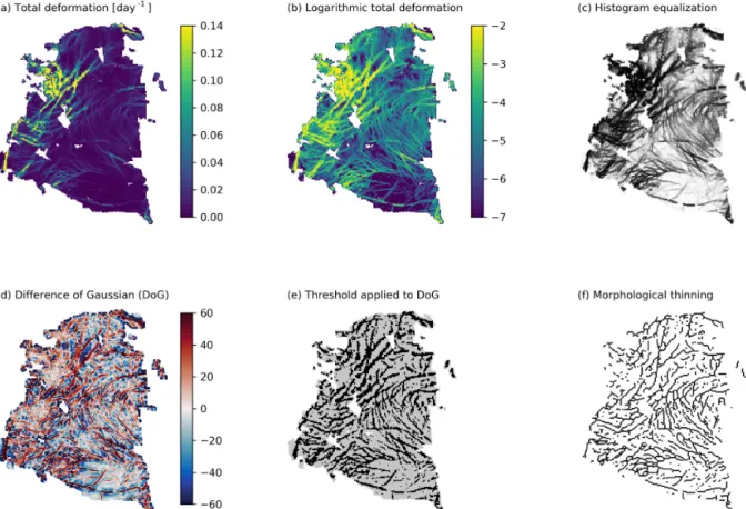
The standard input data of the LKF detection algorithm is the total deformation rate of sea ice˙_tot=

q

˙²_I+ ˙_II², where˙_Iis the divergence and˙IIthe shear that can be derived from both satellite data and model output (Fig. 1a). LKFs are defined by regions of high deformation rates because they are lo- cated along the boundaries of ice floes where most deformation takes place. The actual magnitude of deformation along an LKF, however, varies with the background deformation and the spatial scale because of its multi-fractal properties (Weiss, 2013). Thus a simple thresholding of deformation rates is not sufficient to filter LKFs. Instead, we are inter- ested in detecting deformation that is notably higher than the local environment. As LKFs are lines of high deformation, we need to detect edges in the deformation field.

Prior to the edge detection, we take the natural logarithm of the input field (Fig. 1b) and perform a histogram equal-

ization (Fig. 1c). Both highlight the local differences across different scales and enhance the contrast in regions of low deformation rates.

We use a difference of Gaussian (DoG) filter following Linow and Dierking (2017) for the edge detection (Fig. 1d).

The DoG filter subtracts two filtered versions of the same input data: the first is smoothed with a Gaussian kernel of radiusr₁=1 pixel corresponding to a half-width σ₁=0.5, and the second is smoothed with a Gaussian kernel of radiusr₂=5 pixels (half-widthσ₂=2.5), wherer₁< r₂. The smaller radius r₁ corresponds to the smallest scale of features that will be detected by the DoG and the second ra- diusr2provides the upper limit of the scales detected. Note that this scale limitation applies to the width of the LKFs as well as to their lengths. For edges of scaler1< L < r2, the DoG-filtered values are positive because the local deformation rate is higher than in the environment of radiusr2. Pixels are marked as LKFs when the DoG-filtered pixels are larger than a positive thresholdd_LKF. The result is a binary map in which pixels with a value of 1 belong to LKFs (see Fig. 1e for a threshold of 15). The thresholdd_LKF does not have a unit as it describes the difference of two histogram-equalized images, for which the highest deformation rate corresponds to a pixel value 255 and the lowest to a value of 0.

At this point, LKFs in the binary map are still represented in their original width. To detect which pixels belong to which LKF we add a further level of abstraction and reduce the width of all LKFs to 1 pixel (Fig. 1f). To this end, a morphological thinning algorithm reduces the binary map to its skeleton. We use theskeletonizefunction of the open-source Python packagescikit-image(van der Walt et al., 2014) based on Zhang and Suen (1984). Skele- tonization was used before to detect leads in original or clas- sified, that is, preprocessed and charted, SAR images (Ban- field, 1992; Van Dyne and Tsatsoulis, 1993; Van Dyne et al., 1998).

3.1.2 Segment detection

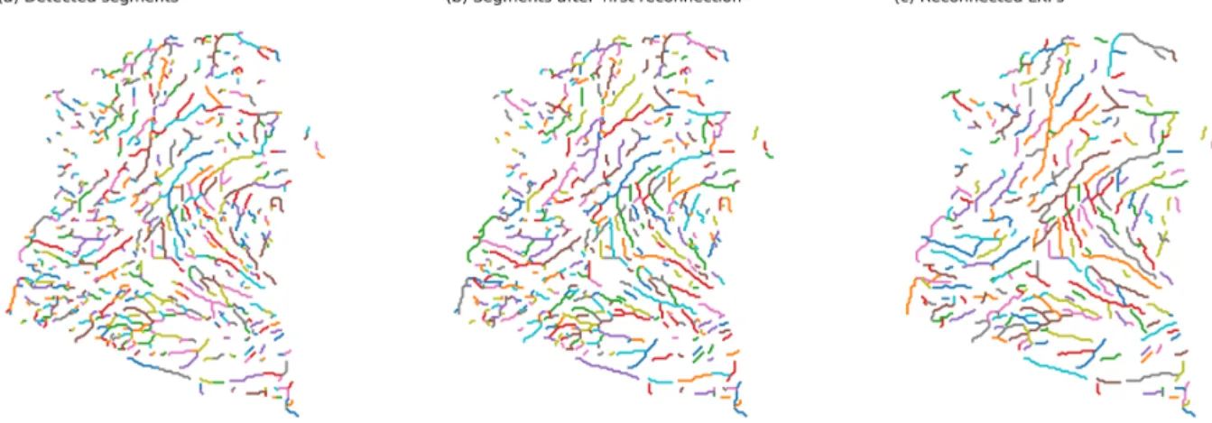
We detect small segments of pixels that contain parts of one LKF in the binary map. Based on the morphological thinned binary map, groups of pixels that form a line are detected. In this first detection step, we want to guarantee that all pixels of a detected segment belong to the same LKF. Therefore, we detect the smallest segments possible that are in the simplest case the points in between intersections of lines in the binary map (Fig. 1f).

As a starting point of the segment detection we use LKF pixels that have only one neighboring cell also marked as LKF. Within each iteration, the detection algorithm proceeds to the LKF neighbor and again checks the number of neighboring cells for LKFs. If the new cell also only has one neighboring LKF cell (neglecting the cell from the prior iteration) the search is continued. If the new cell has more than one neighboring LKF cell, that is, it is a junction, the detection

(4)

Figure 1.Filter sequence from(a)input field total deformation to(f)final output of the morphological thinned binary map of LKF pixels.

Intermediate steps are(b) logarithmic deformation,(c)histogram equalization,(d)difference of Gaussian filter, and(e)the thresholded output of the DoG filter. RGPS deformation data for 1 January 2006 are used for this example.

cycle is stopped and these neighboring points become the new starting points. In addition to the number of neighboring LKF cells, a change in direction compared to the orientation of the last 5 pixels can also terminate the detection cycle: if the angle between the line connecting the centers of the po- tential new cell and the current cell and the linear fit to the previous 5 pixels of the segment exceeds 45^◦, the detection cycle is interrupted and the new cell is marked as a new starting point. If the segment is still shorter than 5 pixels, all available pixels are taken into account. We use 5 pixels in contrast to 2 pixels used by Linow and Dierking (2017) to impose a stronger constraint on the curvature. As in the 2 pixel case, a 90^◦shift of direction is possible within two steps of the detection. Within each cycle of the detection algorithm, pixels that have been assigned to a segment are removed from the input binary map to prevent double assignments. This procedure is repeated until no new starting cells are found.

After removing all linear segments, the remaining binary map contains only non-LKF pixels or LKFs forming closed contours with no starting points. The closed contours are opened by arbitrarily marking pairs of two neighboring LKF pixels (every (i·100)th and (i·100+1)th LKF pixel for i=1,2,3, . . .) as starting points. Then the segment detection is repeated until no new starting points are found. The ini-

tialization step to open closed contours is then repeated until all LKF pixels in the binary map are assigned to a linear segment. All segments that were detected are shown in Fig. 2a for 1 January 2006.

3.1.3 Reconnection

The reconnection instance is designed to connect multiple detected segments that belong to the same LKF. Two segments belonging to the same LKF should have a similar orientation and deformation magnitude and they should be in close proximity to each other. Thus, we compute the probability for all possible pairs of segments to be part of the same LKF based on their distance, their orientation, and their deformation rates. The two segments of the pair with the highest probability are connected and the probabilities of pairs containing one of the two are updated. These steps are iterated until no new matches are found. This part of the algorithm represents a new feature compared to Linow and Dierk- ing (2017).

The central element of the reconnection step is the probability matrixP∈IR^N×N that stores the probabilities for all pairs of segments withN being the number of segments. The rows and columns correspond to single segments, for which

(5)

Figure 2. (a)Detected segments and the results of(b)the first reconnection step and(c)the second reconnection step for RGPS deformation data from 1 January 2006. Each color denotes a different segment or LKF. Due to a limited number of colors, different segments or LKFs can have the same color. The output of the second reconnection step is the final output of the LKF detection algorithm.

P(m, n)gives the probability of segmentmandnbeing part of the same LKF. The probability is given by

P(m, n)= s

1D (m, n) D0

2

+

1O (m, n) O0

2

+

1log₁₀ (m, n)˙ ˙₀

2

, (1)

with the elliptical distance1D between the two segments, the difference in orientation1O, and the difference of the logarithm of the total deformation rate1log₁₀. Here we use˙ the common logarithm, i.e., log base 10, in contrast to the natural logarithm used in Sect. 3.1.1 to directly describe the difference in the order of magnitude in the total deformation of two segments. The difference in orientation 1O is determined by the angle between the two segments, which are represented in this computation by a line connecting the start and the end point. The elliptical distance describes the distance between both segments, but also takes into account the alignment of the segments. In doing so, we decompose the vector connecting both ends of the segments v_a→b into an orthonormal basis with one vector parallel to the first seg- mentakand one vector perpendicular to ita⊥as shown in Fig. 3. In the same way,v_b→ais decomposed into a basis for the second segmentb_k,b_⊥,

v_a→b= a_k,a_⊥

·α =^! v_b→a= b_k,b_⊥

·β, (2) where α and β are the coefficients of the vector decom- position. In the computation of the length of the connecting vector v, the component perpendicular to the segment is weighted with an elliptical factor e >1 and the distance computed by both bases is averaged to obtain a symmetrical elliptical distance, that is,v=v_a→b=v_b→a:

kvk_e=1

2(kv_a→bk_e+ kv_b→ak_e)

=1 2

s α^T·

1 0 0 e

·α+ s

β^T · 1 0

0 e

·β

!

=1D. (3)

We consider only pairs of segments in which the starting point of one segment lies in the direction of the other segment, that is, α (0)≥0 or β (0)≤0. Thus points with the same elliptical distance lie on a half ellipse centered at the endpoint of the segment as denoted in Fig. 3. The computed probability for a generic pair of segmentsP(m, n)=P(n, m) is symmetric, because both the elliptical distance, the orientation difference and the deformation rate difference are symmetric. Thus, we only computeP(m, n)withm < n, where Pis simplified as an upper diagonal matrix.

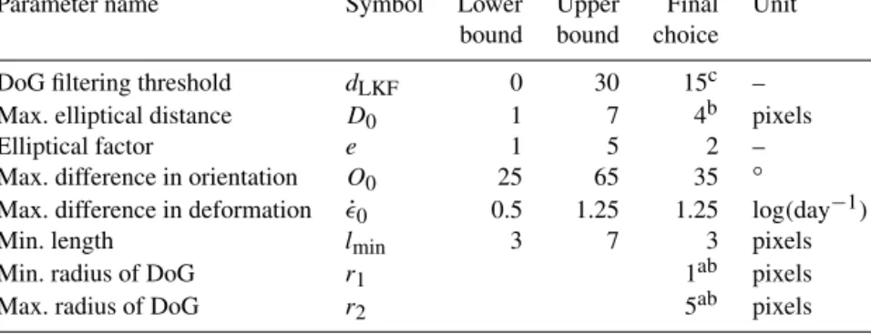
The parametersD₀,O₀, and˙₀not only normalize the individual components of Eq. (1) but also serve as an upper threshold for these components. If for one pair the elliptical distance1D, the difference in orientation1O, or the deformation rate1˙exceeds the thresholdD0,O0, and˙0, it is not considered for the reconnection. The threshold values will be determined in Sect. 3.1.4 and are given in Table 1.

After initializing the matrix P, the pair of segments with the highest probability P(m, n)is connected and the connected segment (m n) replaces the old segment m.

Thereby the number of segments is reduced by one and the nth row andnth column are removed from the probability matrixP. The elements of the probability matrix that correspond to the segmentsmneed to be updated and thus themth row andmth column ofPare reevaluated based on the new connected segment (m n). This process is iterated, and in each iteration the pair of segments with the highest probabil-

(6)

Table 1.List of parameters used in the LKF detection algorithm. For each parameter the lower and upper bounds of the optimization are given along with the final choice of the parameter value.

Parameter name Symbol Lower Upper Final Unit

bound bound choice

DoG filtering threshold dLKF 0 30 15^c –

Max. elliptical distance D₀ 1 7 4^b pixels

Elliptical factor e 1 5 2 –

Max. difference in orientation O₀ 25 65 35 ^◦

Max. difference in deformation ˙₀ 0.5 1.25 1.25 log(day⁻¹)

Min. length l_min 3 7 3 pixels

Min. radius of DoG r₁ 1^ab pixels

Max. radius of DoG r₂ 5^ab pixels

aParameters that have not been optimized but taken from Linow and Dierking (2017).^bParameters are related to length scales and need to be scaled with the spatial resolution of the input data.^cParameters are used to suppress noise in the input data and need to be adapted individually to input data.

Figure 3.Sketch of two segmentsAandBillustrating the principle behind the elliptical distance. In the distance computation the component pointing in the direction perpendicular to the segment is weighted by a factor ofe. Within the shaded area the elliptical distance is below a thresholdD₀. If the endpoints of both segments lie within the area where both shaded half ellipses overlap, they are considered for reconnection. The dotted lines indicate the orientation of lines connecting the start and end points of both segments and the angle 1O is the difference in orientation.vis the vector connecting the endpoints of both segments as defined in Eq. (2).

akanda⊥are basis vectors aligned in the direction of segmentA, respectivelyb_kandb_⊥forB.

ity is connected, until no pair is left that satisfies the threshold valuesD0,O0, and˙0.

In the final step of the LKF detection algorithm, features that fall below a minimum length lmin are removed because most small features are artifacts of the thinning algorithm and do not represent LKFs. With increasing minimum length, the number of detected LKFs decreases and the field of the detected LKFs shows a higher degree of abstraction. The minimum resolution of the detected LKFs, however, is determined by the minimum length used for the DoG filtering. The presented reconnection procedure shows better results for longer segments because the orientation and mean deformation is more sensitive for smaller segments.

In theory, the best input would be segments containing all the points in the binary map that lie in between “junctions”

of the lines, assuming that all those points belong to the same LKF. The segment detection instance, however, yields smaller segments due to the parallel detection that has been implemented to increase computational efficiency. Thus, we apply the reconnection algorithm twice: the first instance is meant to compensate for the tendency of the segment detection algorithm to divide segments into smaller pieces although they actually belong to the same inter-junction segment. Thus, we use very a restrictive set of threshold values (maximum distanceD₀=1.5 pixels, maximum difference in orientationO₀=50^◦, maximum difference in deformation rate˙₀=0.75 log (day⁻¹), elliptical factore=1, and minimum lengthl_min=2 pixels) to ensure that only segments are reconnected that are not separated by more than 1 pixel and no segments are removed because they are short (Fig. 2b).

The second reconnection instance with a different set of parameters is then used to reconnect segments across junctions and to generate the final LKFs shown in Fig. 2c. The choice of the set of parameters used in the second reconnection instance is discussed in Sect. 3.1.4.

3.1.4 Parameter selection

There are a number of parameters in the detection algorithm.

For some of them the range of possible choices can be nar- rowed down with information from field and satellite observations as well as theory of ice fracture, but none of them are strictly constrained. Therefore, we attempted an optimization of the set of parameters, mainly of the reconnection step, given in Table 1.

The main challenge of the optimization is the strong nonlinearity of the detection algorithm. The main source of nonlinearity is the fact that whether a feature is detected or not can depend sensitively on small changes of a parameter. An- other source of nonlinearity is the small number of reference data. The strong nonlinearity of the problem constrains both the definition of the cost function and the optimization

(7)

method to make sure that the optimized solution is the global minimum of the cost function.

We constructed different cost functions, ranging from simple counts of falsely undetected features by the algorithm to a cumulative modified Hausdorff distance (MHD) between all detected and handpicked features as a cost function, in an effort to smooth the strong nonlinearity. In addition, we used different nonlinear optimization routines including basin-hopping (Wales and Doye, 1997) and a nested brute- force implementation. No combination of cost function and optimization method leads to a satisfying result because in all cases the cost function was very sensitive to smaller variations in the parameters. We concluded that finding a global minimum of the cost function is impossible. Therefore, we use a set of parameters estimated with a simple brute-force algorithm that minimizes the number of not-detected features for the range of parameters given in Table 1, in which for each parameter five equally spaced values within its range are used. We do not regard this set of parameters as the global optimum but rather as a useful working basis given the strong nonlinearity of the problem and the limited number of reference data. The performance of the detection algorithm with this set of parameters is evaluated in detail in Sect. 3.2.

3.2 Evaluation

In the evaluation we use all data for January 2006 (11 snapshots) from the handpicked LKF data set, the LKFs detected by the algorithm presented in this study, and LKFs detected by the original version of this algorithm (Linow and Dierk- ing, 2017). The reference data of the original algorithm are generated with the parameters used in the evaluation section of Linow and Dierking (2017). In this way, we evaluate the overall ability of the method to properly detect LKFs but also check whether the modifications and new additions improve the performance of the algorithm. We determine to what degree the algorithms can detect the same features that were recognized by visual inspection and furthermore provide de- tailed information about the similarity and differences between automatically detected and handpicked features in an element-wise comparison.

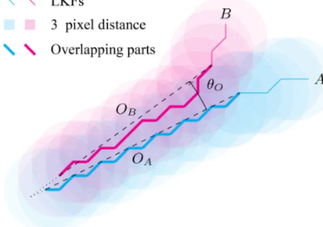
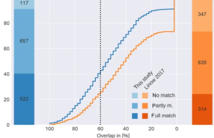
The principal idea behind this evaluation is that we compare the features pairwise: one LKF from the handpicked data with the best-matching automated detected LKF. We find the best matching automatically detected feature for each handpicked feature by minimizing the MHD (Dubuisson and Jain, 1994) between the handpicked features and all automatically detected features. Next, we categorize all pairs by the degree of overlap of the handpicked feature with its closest matching detected feature. The overlap between two features is illustrated in Fig. 4. The number of pixels for which the distance to the closest pixel in the matching feature is smaller thand_O=3 pixels is defined as overlap, labeled asO_Aand O_B in Fig. 4. To distinguish between the overlap of feature pairs that have a similar shape but are displaced and pairs that

Figure 4.Illustration of overlap between two LKFsAandB.

overlap only due to intersection of both features, we compute the angle between overlapping parts of the matching pairsθO. If this angle is smaller thanθ_O<25^◦, the overlap of a matching pair is defined by the minimum of overlapping pixels of both matching partners normalized by the maximum length of both matching partners:

O=min(len(O_A),len(O_B)) /max(len(A),len(B)) ,

for θO<25^◦. (4)

Given this definition of overlap, we distinguish among three different classes of pairs: (1)fully matching pairsthat have an overlap larger than 60 %, (2)partly matching pairs that have an overlap smaller than 60 % but larger than 0 %, and (3)not matching pairswith overlap equal to 0 %.

The overall performance of the algorithm with respect to the overlap of the detected features with the reference data set is given in Fig. 5 along with the number of pairs within each class. We find that the features detected with our new algorithm overlap significantly more with the handpicked reference data than the features detected with the original version of the algorithm (Fig. 5). The original version of the algorithm is run with the same parameters used in the evaluation section of Linow and Dierking (2017). Our modifications to the algorithm increase the number of fully matching LKFs by 66 % (from 314 to 522), along with a similar number of partly matching LKFs (from 635 to 657) and a clear decrease of 66 % for the not matching LKFs (from 347 to 117). This indicates a significant improvement of the original algorithm.

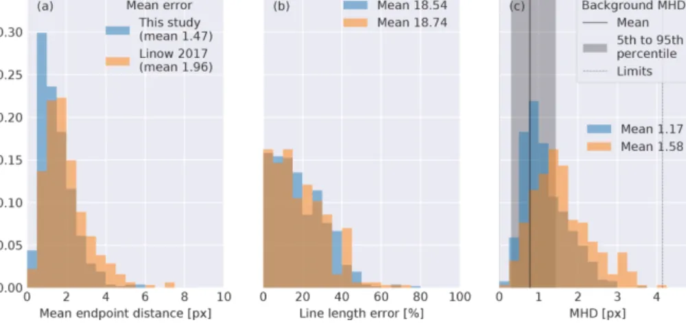
We analyze the similarity of features of all pairs within each class to test whether these improvements are made at the expense of the quality of the detected features. In doing so, we define three metrics to determine the similarity of the features: (1) the mean endpoint distance, (2) the line length error, and (3) the MHD as metrics, at which the first two were introduced by Linow and Dierking (2017). The MHD is a measure of the general agreement of two shapes. It takes into account changes in both orientation and length but also a complete change in shape. In the sea ice context, the MHD is

(8)

Figure 5.Evaluation of the detection algorithm presented in this study and the original algorithm (Linow and Dierking, 2017) against handpicked LKFs. The cumulative frequency of occurrence of the overlap is given in the center plot. The number of features is given in the bar plots for each class (fully matching, partly matching, and not matching).

applied, for example, to evaluate the ice edge position in sea ice forecasts (Dukhovskoy et al., 2015) or to assess the pre- dictability of LKFs (Mohammadi-Aragh et al., 2018). Here we only focus on the class of full matching pairs.

For the mean endpoint distance, we determine the distance between both endpoints of the detected and the handpicked features for each pair and average them. For all full matching pairs with features detected by our new algorithm the endpoint distance tends to be smaller compared to features detected by the original version of the algorithm, which is indicated by the shift in the distribution towards smaller errors (Fig. 6a). The improved match because of the modifications to the original algorithm is also reflected in the smaller mean error (1.47 pixels as opposed to 1.96 pixels of the original algorithm). For 75 % of the features detected with our algorithm, the mean endpoint distance is smaller than 2 pixels whereas this is only the case for 60 % of features detected by the original version.

The line length error is determined by the difference in length of the two features in a pair normalized by length of the smaller feature of the pair. For both algorithms, the distributions are similar with similar mean errors of∼18 % (Fig. 6b). For half of the pairs the line length error is also lower than 15 % in both cases.

We find that our modifications to the original algorithm also reduce the average MHD from 1.58 to 1.17 pixels (Fig. 6c). A total of 73 % of these pairs lie within the fifth to 95th percentiles of the background MHD defined as the MHD of the reference data and the morphological thinned binary LKF field (Fig. 1f). Since all LKFs consist of sets of pixels from this binary field, the background MHD is an upper limit of how accurate a reconnection algorithm can become using this binary field as an input value.

In conclusion our new version of the algorithm improves the original algorithm in that it detects more features and also increases their agreement with the handpicked reference data.

3.3 Discussion

Our adapted detection algorithm greatly improves the original version. The total number of handpicked features that is reproduced by the algorithm increased by 66 %. In addition, the quality of the detected features with respect to their mean endpoint distance, the error in line length, and the MHD is improved. We attribute these improvements to two changes that stand out in addition to smaller adjustments in the code: (1) the introduction of a probability-based reconnection and (2) the optimization of the DoG thresholddLKF, which showed the highest sensitivity in the optimization. We use this threshold to filter LKFs as regions that have high deformation rates compared to the local environment. The deformation rates in RGPS are known to be prone to grid- scale noise and uncertainties caused by tracking and geoloca- tion errors (Lindsay and Stern, 2003; Bouillon and Rampal, 2015), which can lead to a false classification of a pixel as LKF. Increasing the threshold slightly suppresses this noise, albeit at the expense of losing features with smaller deformation rate differences. Thus the threshold needs to be optimized to balance both effects; we founddLKF=15 to be the best parameter choice for the RGPS data set.

In our algorithm we reconnected segments to LKFs based on a probability computed from the characteristics of the segments. Thereby those segments that fit “the best” are reconnected, and in contrast to Linow and Dierking (2017) the reconnection does not depend on the order in which the reconnection algorithm runs over the list of segments. In doing so, we improve the quality of the detected features and obtain a unique and consistent solution. Both uniqueness and consistency are necessary ingredients for the ensuing application of a tracking algorithm.

In this context, we found the elliptical distance1D and the orientation1O to be the important contributors to the probability function. The optimized threshold 1˙0=1.25 for differences in deformation rates is very high (as it is applied to the difference of the common logarithm of the deformation rates, a difference between deformation rates of a factor 10^1.25=17.78 is possible), so that differences in deformation rates are normalized by a large value and do not contribute much to the probability function. Omitting the deformation-related part in Eq. (1) (equivalent to set- ting1˙₀= ∞) does not change the results of the evaluation of the optimized solution very much (not shown here). The small influence of the threshold for deformation rates1˙₀ on the performance of the algorithm may also be caused by the noise in the RGPS data along LKFs (Bouillon and Ram- pal, 2015). Smaller segments, especially, are affected by the

(9)

Figure 6.Statistics of all full matching pairs computed for the algorithm presented here and the original version (Linow and Dierking, 2017):

(a)the mean endpoint distance,(b)the line length error, and(c)the modified Hausdorff distance (MHD). The background MHD refers to MHD calculated for the handpicked features and the morphological thinned binary field (Fig. 1f).

noisy RGPS data so that segments that belong to the same LKF may have different deformation rates.

4 LKF tracking

The dynamic nature of the ice pack with spontaneous fracture, fast propagation of failure lines, and discontinuous drift fields makes tracking of deformation features in the ice a challenge. Because most of these processes occur on timescales from seconds to days, the temporal resolution of the RGPS data set of 3 days makes feature tracking even more challenging. In this section, we present an algorithm that automatically tracks features and we compare the tracked features to hand-tracked features.

4.1 Method description

The tracking of deformation features, in fact any feature, between two time records is always a two-step problem: first, the deformation features are detected for both records sepa- rately and, second, the features of both time records are connected in time by identifying features of the first record with those of the second record.

Between two RGPS time records (3 days) a deformation feature will be advected and can undergo the following changes: (1) it can become inactive, (2) it can shrink, or (3) it can undergo a combination of growing and shrinking.

Thus, on top of two time records, tracking requires drift information between these records. From the same drift fields that were used to derive the deformation data we estimate a first-guess position of each feature from the first record in the second record that neglects all effects but advection. We compute the drift first-guess position in pixel space (each feature in the first record is described by integer pixel indices) by normalizing the drift speed with the grid resolution. Thus,

the computed first-guess positions are given in floating point indices of the input field of the detection algorithm.

For the following description, a tracked feature is a feature from record two with an associated feature in record one; a matching pair is a pair of associated features from records one and two; and all matching pairs are called the tracks.

A tracked feature in the second record is required to overlap at least in part with the first-guess position after growing and shrinking in between the time records is taken into account. We define a search window around the first-guess position of the feature to test for an overlap of the features with the first-guess position. The search window consists primar- ily of pixels for which the floating point indices of the first- guess position are rounded up and down by the Python func- tionsceil andfloor. To take into account the position uncertainty caused by the morphological thinning algorithm, we also add all neighboring pixels of the pixels with rounded indices using the mean background MHD of the morphological thinned field (Fig. 6c) of 0.78 pixel as an estimate for this uncertainty. All features in the second record that include a minimum number of pixelsomin=4 of the search window are marked as potentially tracked features. If we consider a feature that changes shape only due to advection without any growing or shrinking, the tracked feature from the sub- sequent time record should lie completely within the search window.

During the course of 3 days, however, many features grow or an opening closes at one or both ends of the detected feature. Also, in rare cases, only parts of a feature close and a new branch is formed within the position of the old feature. This will be referred to as branching. Our algorithm is designed to take into account only growing and shrinking because in our experience there are rather few branching LKFs (10 %) and because branching is very complex to track. Thus, a feature that is considered as a tracked feature is allowed to grow at both ends compared to the first record or to shrink

(10)

to only a part of the original feature. To translate this into an algorithm, we define a search area that is the area enclosed by two lines through the endpoints of the first-guess position.

These lines are perpendicular to the orientation of the first- guess position (see grey shaded area Fig. 7). For a tracked feature, all points of this feature that lie within the search area need also to lie within the search window. Here, we im- plement a threshold valuep_w/a that defines the fraction of points within the search window and points within the search area for the feature to be considered as a tracked feature. Fea- tures, for which more pixels lie within the search area but not in the search window, have likely undergone branching or just intersect with the first-guess position but have a different orientation.

The last step of the tracking algorithm filters small features inside the search window that intersect with the first-guess position. Due to their short length all of their points in the search area also lie in the search window. To exclude those we compute the overlap as defined in Sect. 3.2 between the first-guess position and the potentially tracked feature. We use a maximum distance of pixels of d_O=1.5 and an angle threshold ofθ_O=25^◦for the computation of the overlap.

All potentially tracked features with a nonzero overlap are marked as tracked features.

For all features of the first record this procedure is repeated iteratively: (1) advect the feature using the drift information to obtain the first-guess position, (2) check for features that shareomin pixels with the search window, (3) compute the fraction of pixels in the search window and in the search area pw/a, and (4) test for nonzero overlap. The output of the tracking algorithm is a list of matching pairs of always one feature from the first record and a tracked feature from the second time record.

4.2 Parameter optimization

In the tracking algorithm the four parameterso_min,p_w/a,d_O, andθ_Oare not very well constrained, so we attempt to optimize them within plausible bounds. As we want to optimize the tracking algorithm independently of the detection algorithm, we use the handpicked features as input for the tracking algorithm and compare the output to the hand-tracked features. We perform the same very basic optimization as in Sect. 3.1.4 facing similar problems with a limited number of reference data and a nonlinear cost function. We choose equally spaced values in the range given in Table 2 for all four parameters and determine the number of correctly tracked features, the missed tracks, and false positives. We find that decreasingo_minand increasingp_w/a,d_O, andθ_Oleads to an increase in correctly tracked features along with a large increase in false positives. To balance both effects, we define the cost function as the number of correctly tracked features subtracted by the number of missed tracks and the number of false positives. The final parameter set that maximizes this difference is given in Table 2.

Figure 7.Principle of the tracking algorithm showing the search area and search window.Ais the original feature (dashed blue) and A_d(blue) the first-guess position considering only drift.B andC are two features in the second record, in whichB is marked as a successfully tracked feature.

4.3 Evaluation

To separate the two steps of feature tracking, and to enable an independent evaluation of the tracking algorithm, we apply the tracking algorithm to two different LKF data sets:

the handpicked features and the features extracted by the detection algorithm for the same time span. Then, we compare both results to the hand-tracked features described in Sect. 2.3.

We evaluate the tracking algorithm independently by applying it to the handpicked features and test whether the algorithm reproduces the hand-tracked features of the next time record, hereafter referred to as “only tracking”. The algorithm picks 336 (85.7 %) of the overall 392 handpicked tracked features correctly and only misses 56 (14.3 %). In addition to the missed tracks, the algorithm detects 89 false positives. We use the information describing the type in change of shape (no change, growing, shrinking, and branching) provided for the handpicked tracks to test the performance of the algorithm for those different types of change (Fig. 8a). The performance of the algorithm ranges from 85 % to 88 % for the different types with the branching type being an excep- tion for which only 56 % of the features are tracked correctly.

This is not surprising as the algorithm is not designed to track this type of change.

In the evaluation of both the detection and tracking algorithms, we distinguish between missed tracks that were not tracked by the tracking algorithm and tracks that were missed because the detection algorithm was not able to detect the corresponding features in both time records. First, we test whether the detection algorithm picks both features of a handpicked matching pair. In doing so, we separate both fea-

(11)

Table 2.List of parameters used in the LKF tracking algorithm. For each parameter the lower and upper bounds of the optimization are given along with the final choice of the parameter value.

Parameter name Symbol Lower Upper Final Unit

bound bound choice

Min. overlap in search window o_min 2 6 4 pixels

Fraction of pixels in search window and in search area p_w/a 0.5 1 0.75 –

Max. distance of pixels for overlap d_O 0.75 2.25 1.5 pixels

Max. angle for overlap θ_O 15 35 25 ^◦

Figure 8.Evaluation of(a)only the tracking algorithm for the handpicked features and(b)a combination of the detection and tracking algorithms. The colored segments of each bar show the different combinations of changes in shape (no change, growing, shrinking, and branching) that are labeled by the black lines next to the bar. The missed tracks in panel(b)are separated into not detected or not tracked features. Above the bars the percentage compared to all handpicked tracks is given for all types and for all types except branching, which is given in brackets.

tures into the parts that both features share and a nonoverlapping part to account for varying shapes in the nonoverlapping part of detected and handpicked features. Then, we check whether detected features correspond to the handpicked features using the overlap as in Sect. 3.2. If for one of the two handpicked features no corresponding detected feature is found, this handpicked tracked feature is marked as a missed tracked feature caused by the detection algorithm. Otherwise, we test whether the tracking algorithm tracks the detected features appropriately. In total, 54.1 % of the handpicked matching pairs are detected and tracked correctly, whereas 21.6 % are not captured by the tracking algorithm, and for 24.4 % of the tracked features the corresponding features are not detected. Interestingly, these fractions do not change significantly if subsampled to individual types of change. Only for the branching type of tracks, the rate of tracked features missed by the tracking algorithm exceeds the one for the detection algorithm, which is in line with the low number of matching pairs captured by the tracking algorithm for this type of change found in the evaluation of the tracking algorithm alone.

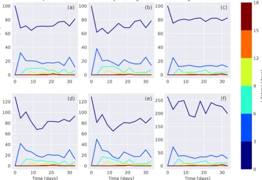
Since not all handpicked tracked features are tracked automatically by the presented algorithm, we need to make sure that this does not change the temporal characteristics of the automatically generated tracked features. In doing so, we compare the distributions of lifetimes (Fig. 9) and growth rates (Fig. 10) of the handpicked tracked features (handpicked), the automatically tracked features of the handpicked features (only tracking), and the automatically tracked features of the automatically detected features (tracking and detection). At the beginning of the evaluation period, all features are initialized with a lifetime in the class of 0 to 3 days, for which the range of the class is given by the temporal resolution of the input data. For the following time steps, all features that are marked as tracked features are assigned to the next lifetime class compared to the class of their tracking partner in the previous time record. All other features are initialized again in the lowest category of 0 to 3 days. For all three different data sets, more than 99 % of features have a lifetime smaller than 12 days, which can be thought of as the average spin-up time needed by the tracking algorithm. In the following, we consider only the period after those 12 days.

(12)

Figure 9.Distribution of lifetime of all features in the first 12 RGPS snapshots in 2006 in the handpicked reference data(a, d), the automatically tracked features of the handpicked features(b, e), and the automatically tracked features of the automatically detected features(c, f).

Panels(a–c)show the absolute number of features for a certain lifetime class, whereas panels(d–f)are normalized by the total number of features for this time record.

Figure 10.Probability distribution function for growth rates in(a)the handpicked reference data,(b)the automatically tracked features of the handpicked features, and(c)the automatically tracked features of the automatically detected features separated into growth for positive growth rates and shrink for negative values.

The distribution of lifetimes for the handpicked tracks and automatically generated tracks of handpicked features are very similar: (1) the number of features in the lowest lifetime category increases in absolute and relative numbers to the end of the evaluation period in an equal manner (70 % to 81 %, handpicked, and 67 % to 78 %, only tracking), (2) 17 % (handpicked) and 18 % (only tracking) of the features have a lifetime of 3 to 6 days, and (3) in both cases the remaining 9 % of the features have a lifetime of over 6 days. In a feature-by-feature comparison for both data sets, only 10 % of the features vary in their lifetime due to uncertainties in

the tracking algorithm. The root-mean-square error of the lifetime is estimated to be 1.55 days. For the automatically detected and tracked features the average lifetime reduces to 3.9 days compared to 4.2 days for the handpicked features, which is driven by an increase in the number of features in the lifetime class 0 to 3 days to 81 %. The fractions of the remaining classes are reduced accordingly but do not change significantly relative to each other.

In addition to the lifetime as the main temporal character- istic, we compute the growth rates of all tracked features to check whether the shape of the tracked features changes in a

(13)

similar manner. The growth rate is defined as the difference of the number of pixels of the feature in the second record compared to the feature of the previous record. In our analysis, we divide the growth rate into two regimes depending on its sign: growth of the feature for positive values and shrinking of the feature for negative values. The distributions of the growth rates for the handpicked, only tracking, and tracking and detection data sets all have an exponential distribution (Fig.10) with half of the features changing by less than 3 pixels per day. The high order of similarity of the distributions indicates that the usage of the detection and tracking algorithms does not distort the characteristics of tracked features, even though the total number of features detected and tracked increases by a factor of 2.3 for the detection and tracking data set.

4.4 Discussion

The large time difference of 3 days between records of the RGPS data set significantly complicates the tracking of deformation features because they change shape and positions on shorter timescales. With this background, the overall percentage of 85.7 % of handpicked tracked features that were correctly identified by the algorithm is more than satisfying.

The missed tracks and the false positives of the algorithm lead to a lifetime RMSE of 1.55 days, which is smaller than the uncertainty given by the 3-day temporal resolution of the input deformation data. The low percentage of correctly identified branching features is also acceptable because they only make up 10 % of all handpicked features. We hypothesize that relaxing the constraints in the algorithm to also track branching features will most likely lead to a strong increase in false positives.

Also, the combination of tracking and detection algorithm reproduces more than half of the handpicked tracks. This exceeds the 40 % of features that were fully detected by the detection algorithm and might hint at a better performance of the algorithm for long-lived features. The handpicking of features and tracks by only one individual also leads to a bias in the reference data. To accurately separate the uncertainty caused by the subjectiveness of the reference data from the uncertainty of the algorithm, more individuals would need to repeat the handpicking procedure, which would exceed the scope of this paper. Small LKFs and LKFs in regions of low deformation, in particular, are harder to catch by eye (Linow and Dierking, 2017), which explains that the automatic detection picks 2.3 times more features than in the reference and the number of tracked features increases by 65 %. We assume that this bias towards small and therefore most prob- ably short-lived features is responsible for the slightly higher percentage of features in the class with the lowest lifetime (0 to 3 days). In addition to this small increase, the distributions of lifetimes for the automatically detected and tracked features are very similar, which suggests that there is no significant cumulative bias caused by the application of both al-

gorithms. This is backed by the similar growth rates observed for both data sets.

5 LKF data set

5.1 Generation of LKF data set

In this section, we introduce a data set of LKFs generated by applying the detection and tracking algorithms to all available RGPS data (Hutter et al., 2019). The RGPS data cover the time from November 1996 to April 2008. Here, we use the available winter data from late freezing season (November–December) to the start of the melt onset (April–

May). The Lagrangian drift information that is also provided in the RGPS data set is interpolated to the regular grid used for the RGPS deformation data to be used as input in the LKF tracking.

First, we apply the detection algorithm with the optimized parameters given in Table 1 to all deformation data. The output of the detection algorithm is a list of LKFs for each time record that includes one array for each LKF. The array stores the position (as an index in the RGPS grid and in latitude and longitude coordinates) and deformation (divergence and shear rate) information of all points of the LKF. Next, we feed the interpolated drift information and the detected LKFs of each year to the tracking algorithm and determine the link- ages between LKFs for successive time records. The tracking algorithm with the optimized parameters given in Table 2 provides a list of tracked pairs. Each pair contains the indices of the LKFs in records one and two.

Overall 164 698 LKFs were detected and 35 855 tracked features were found. The yearly detection numbers range from 11 002 LKFs for winter 2006/07, the year of a sea ice minimum, to 16 774 LKFs in winter 2001/02. If the number of detected features is normalized by the number of observations of sea ice deformation, we find the maximum to be in winter 1996/97 and the minimum in 2002/03. The number of tracks varies from 2012 tracks in winter 2003/04 to 4127 tracks in winter 2001/02.

The deformation, more precisely the divergence rate, which is saved for each LKF, can be used to distinguish leads from pressure ridges in the generation of an LKF. In general, leads form in divergent ice motion and pressure ridges in convergent ice motion and the converse of this relation can be used to label newly formed LKFs. Persistent LKFs can also be labeled in this way, as long as the sign of divergence does not change during the lifetime of an LKF. Consider an LKF, initially labeled as a lead in divergence, that encounters convergent motion. Depending on the magnitude of conver- gence, the lead may either only partly close and continue to be an open lead, or it may close completely and even evolve into a pressure ridge, making differentiating between leads and ridges difficult. Thus, we refrain from labeling all LKFs in the data set into leads and pressure ridges but provide the

(14)

deformation rates for each LKF and leave this classification and its evaluation to the informed user. As an approximate first guess, we estimate that 46 % of the LKFs in the data set are leads, 41 % are pressure ridges, and 13 % are unclassified (because the associated mean divergence rate along the LKF changes sign over the lifetime of the LKF). For the classi- fied leads and pressure ridges the sign of divergence does not change over the lifetime. Please note that these estimates, especially for short LKFs, are likely contaminated with grid- scale noise in the divergence data of RGPS (Lindsay and Stern, 2003; Bouillon and Rampal, 2015). Combining the LKF data set with sea ice thickness and concentration data would allow us to clearly distinguish between leads and pressure ridges by using these additional constraints: (1) along a lead the sea ice concentration decreases within the time step, and (2) along pressure ridges the sea ice thickness increases.

5.2 Applications and discussion

In this section, we present a few illustrative statistics of the LKF data set. In doing so, we intend to demonstrate the use- fulness of the data set but also to check it for consistency with other studies on leads and sea ice deformation. The statistics (Fig. 11) range from spatial properties such as LKF length, LKF density, and intersection angles to temporal properties such as LKF lifetimes. In the case of the intersection angle, we give an example for a model–observation comparison with the presented algorithms by comparing the RGPS LKF data set to LKFs that were detected and tracked in a 2 km model simulation with a numerical sea ice ocean model.

In addition, we link the number of deformation features and their corresponding deformation rates to atmospheric drivers, in particular to Arctic cyclones.

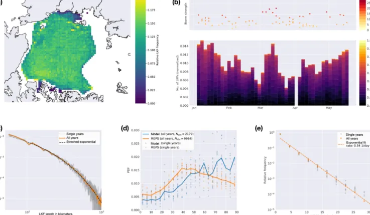
The density of LKFs is computed for the all years of the LKF data set as the incidences when a pixel is crossed by a LKF normalized by the overall number of RGPS observations for this pixel. In Fig. 11a only pixels that have more than 500 RGPS observations are shown. We observe a fairly homogeneous LKF density throughout the entire Amerasian Basin, with a slight increase in the Beaufort Sea. The fast ice regions in the East Siberian Sea have the lowest densities with the fast ice edge showing up as a sudden increase in LKF density. The highest LKF densities are found around the New Siberian Islands, Wrangel Island, and at the coastlines along the Beaufort Sea. This agrees very well with studies on lead densities derived from MODIS thermal-infrared imagery (Willmes and Heinemann, 2016) and CryoSat-2 data (Wernecke and Kaleschke, 2015) that show high densities in the Beaufort Sea and the highest values close to the coastline.

A direct comparison of density values is not possible as those studies are limited to leads that are identified as an opening in the ice cover, whereas our algorithm picks regions of high deformation rates that can also include pressure ridges.

The distributions of LKF length of all single years are very similar and range from∼50 to 1000 km (Fig. 11c). For

LKF lengths between 100 and 1000 km, a stretched exponential,p (x)=Cx^β⁻¹e^−λx^β withC=βλe^λx^min^β (Clauset et al., 2009), accurately describes the probability density function.

The parametersβ=0.719 and λ=0.0531 are determined by numerically finding the maximum likelihood estimate.

We perform a goodness-of-fit test for power-law-distributed data that is based on the Kolmogorov–Smirnov (KS) statis- tic, which is the maximum distance between the cumulative distribution functions (CDFs) of two different distributions (Clauset et al., 2009). We draw random samples from the fitted distribution and compute the KS of the random samples and the fitted distribution. This simulation is repeated 1000 times. We find that the KS of the observed length scales is smaller than the 95 % percentile of the random samples and thereby the observed LKF lengths are described by the fitted distribution. The stretched exponential distribution be- longs to the family of heavy-tailed distributions and is the transition of an exponential and a power-law distribution. It describes many natural phenomena that are dominated by ex- treme events but in contrast to a power-law distribution have a natural upper limit scale (Laherrère and Sornette, 1998).

We limit the range of the fit to 1000 km due to the varying coverage and especially smaller gaps in the RGPS data that might divide long features into multiple smaller segments. We set the lower bound to 100 km to account for the discrete character of the LKF length that disturbs the distribution at lower LKF lengths. As LKFs here are collec- tions of pixels, their length is set by a linear combination of

i+

√ 2j

·12.5 km withi, j∈N.

The intersection angle between two deformation features formed at a similar time is related to the rheology describing the deformation of sea ice. From satellite imagery in the visible range for 14 days in 1991, the intersection angle was found to range between 20 and 40^◦ (Walter and Overland, 1993), which can be linked to the angle of internal friction using a Mohr criterion for failure (Erlingsson, 1988). The distribution of intersection angles of two LKFs that formed in the same time record is given in Fig. 11d, in which only LKFs larger than 10 pixels=125 km are taken into account to reduce the effect of a preferred direction (45 and 90^◦) orig- inating from the rectangular grid. We perform this analysis on the RGPS LKF data set and LKFs that were detected in a 2 km Arctic numerical model simulation, whose details are given in Appendix A. For the RGPS data, we find that the distribution peaks at an angle of 40–50^◦. Angles larger than 50^◦occur more often than angles below 40^◦, and angles between 0 and 20^◦have the lowest occurrence. The broad distribution indicates that there is not only one specific fractur- ing angle but that heterogeneities in the ice cover and tem- perature variations (Schulson, 2004) as well as the dilatancy effect (Tremblay and Mysak, 1997) may influence the deformation on an Arctic-wide scale. The LKFs in the model simulation intersect at larger angles with local maxima in the range of 60 to 90^◦. The difference in the sample size might

(15)

Figure 11.Statistics on LKF data set:(a)LKF density computed for the all years of the data set.(b)Time series of the number of LKFs separated by their deformation rates for winter 2002/03. The number of LKFs is normalized by the number of available pixels for each RGPS time record. For early April no RGPS data are available. For each time record all cyclones (Serreze, 2009) over the Arctic ocean are each shown as a dot in the upper panel. Theyaxis and the color code of the dots in the upper panel provide the local Laplacian of each cyclone as a proxy for its strength.(c)PDF of LKF length along with stretched-exponential fit for LKFs larger than 100 km and smaller than 1000 km.

(d)Intersection angle of pairs of features that are newly formed (lifetime between 0 and 3 days) and have a size of at least 10 pixels for the RGPS and a 2 km Arctic numerical model simulation.(e)Distribution of LKF lifetimes for all years along with a fit to an exponential tail.

cause these strong variations for larger angles, as we find 5 times fewer features in the model simulation than for RGPS within the same period of time. In general, the model under- estimates the probability of intersection angles smaller than 55^◦ and overestimates those of angles larger than 55^◦. We attribute these differences to the usage of the elliptical yield curve with normal flow rule in the simulation because this yield curve does not have a “preferred” direction of fracture in contrast to yield curves with a Mohr–Coulomb criterion.

The intersection angle may be improved by an appropriate choice of model parameters (Ringeisen et al., 2018).

The distribution of lifetimes determined by the tracking algorithm shows an exponential tail with a rate parameter of 0.34 day⁻¹(Fig. 11e). Kwok (2001) described some LKF systems that were persistent in the Arctic over a period of a month for the winter of 1996/97. We also find lifetimes as high as this but show that the majority of LKFs are ac- tive in much shorter time intervals. We assume that the rapid changes in external forcing (mainly wind stress) are the rea- son for the high number of short-lived LKFs.

Last, we study the link between the detected features and the wind forcing being the main driver of ice fracture. To do so, we combine a data set of cyclones in the Northern Hemisphere (Serreze, 2009) with the distribution of LKFs in different deformation rate classes for, as an example, the winter of 2002/03 (Fig. 11b). In the freezing season, we find more deformation features (with generally higher deformation rates) caused by the thinner and therefore weaker ice during this period. With thicker ice the number of deformation features decreases followed by an increase from April onwards, which we attribute to the onset of melting and the resulting weakening of the ice. This overall seasonal cycle is interrupted by a set of four strong cyclones that pass through the Arctic Ocean in March and lead to a sudden increase in the number of deformation features. This confirms that weather systems with high wind speeds are a main driver of sea ice deformation in the Arctic Ocean. The deformation rates associated with the LKFs co-vary with the seasonal cycle of the number of LKFs, which is in agreement with the seasonal cycle of the mean deformation rate (Stern and Lind- say, 2009).