Impact of Poleward Moisture Transport from the North Pacific on the Acceleration of Sea Ice Loss in the Arctic since 2002
H. J. LEE,aM. O. KWON,aS.-W. YEH,bY.-O. KWON,cW. PARK,dJ.-H. PARK,e Y. H. KIM,fANDM. A. ALEXANDERg
aDepartment of Ocean Science, Korea Maritime and Ocean University, Busan, South Korea
bDepartment of Marine Sciences and Convergent Technology, Hanyang University, Ansan, South Korea
cWoods Hole Oceanographic Institution, Woods Hole, Massachusetts
dGEOMAR Helmholtz Centre for Ocean Research Kiel, Kiel, Germany
eDepartment of Ocean Science, Inha University, Incheon, South Korea
fKorea Institute of Ocean Science and Technology, Ansan, South Korea
gNOAA/Earth System Research Laboratory, Boulder, Colorado
(Manuscript received 20 June 2016, in final form 17 May 2017) ABSTRACT
Arctic sea ice area (SIA) during late summer and early fall decreased substantially over the last four de- cades, and its decline accelerated beginning in the early 2000s. Statistical analyses of observations show that enhanced poleward moisture transport from the North Pacific to the Arctic Ocean contributed to the accelerated SIA decrease during the most recent period. As a consequence, specific humidity in the Arctic Pacific sector significantly increased along with an increase of downward longwave radiation beginning in 2002, which led to a significant acceleration in the decline of SIA in the Arctic Pacific sector. The resulting sea ice loss led to increased evaporation in the Arctic Ocean, resulting in a further increase of the specific hu- midity in mid-to-late fall, thus acting as a positive feedback to the sea ice loss. The overall set of processes is also found in a long control simulation of a coupled climate model.
1. Introduction
One of the striking features of recent climate change is a loss of multiyear sea ice in the Arctic, which has been associated with global warming (e.g.,Serreze et al. 2007;
Comiso et al. 2008;Stroeve et al. 2012). Warmer air temperatures caused by increasing greenhouse gas concentrations can accelerate the summer sea ice loss through an ice-albedo feedback as the sea ice gets thinner (Stroeve et al. 2012;Vihma 2014). It has been hypothesized that the sea ice decline caused a significant change in the weather and climate variability in the midlatitudes through a complex set of physical processes (Francis and Vavrus 2012;Hopsch et al. 2012). For in- stance, the sea ice loss can drive local warming in the Arctic atmosphere, which subsequently modulates Rossby wave propagation from the polar region to midlatitudes (Honda et al. 2009; Overland and Wang 2010;Jaiser et al. 2012;Kim et al. 2014;Kug et al. 2015), including planetary waves emanating from the Barents
and Kara Seas to Eurasia (Strong et al. 2009;Deser et al.
2010). Furthermore, Arctic sea ice loss has the potential to enhance the occurrence of the negative phase of the Arctic Oscillation (AO) and even impact the tropics and Southern Hemisphere (Deser et al. 2015).
In addition to ice-albedo feedback, both local and remote factors may contribute to ‘‘Arctic amplification’’—
stronger warming over the Arctic relative to the rest of the globe (Graversen et al. 2008;Screen and Simmonds 2010; Screen et al. 2012). For example, poleward- propagating Rossby waves excited by tropical con- vection lead to Arctic warming through enhanced downward infrared radiation and inducing sinking motion (adiabatic warming) over the Arctic, resulting in the sea ice loss (Lee et al. 2011a,b).Screen and Francis (2016)further found that the contribution of sea ice loss to wintertime Arctic amplification is enhanced during the negative phase of the Pacific decadal oscillation (PDO) relative to the positive phase.
Since satellite-based sea ice observations began in the late 1970s, the Arctic experienced record- breaking minimum sea ice area (SIA) in 2007 and 2012
Corresponding author: Dr. Ho Jin Lee, hjlee@kmou.ac.kr DOI: 10.1175/JCLI-D-16-0461.1
Ó2017 American Meteorological Society. For information regarding reuse of this content and general copyright information, consult theAMS Copyright Policy(www.ametsoc.org/PUBSReuseLicenses).
(Zhang et al. 2008,2013). Several different processes may contribute to these years with below normal sea ice extent.
Graversen et al. (2011)suggested enhanced convergence of warm and humid air into the Arctic was responsible for the extreme loss of sea ice during the summer of 2007.
Increased ocean heat transport through the Bering Strait may also play a role in the dramatic sea ice melting (Wang et al. 2009;Woodgate et al. 2010). In addition, a change in the local Arctic atmospheric circulation (e.g., the Arctic dipole anomaly in recent years) may enhance the sea ice export through the Fram Strait (Overland and Wang 2010;
Tsukernik et al. 2010;Proshutinsky et al. 2015).
The Arctic Pacific sector (APS;Fig. 1a) showed a re- markable decline of SIA in the last decade during August–October (ASO), the end of sea ice melting
season (Figs. 1a,b; see alsoFig. 2a). The rate of decline during 2002–12 is20.0433106km2yr21, roughly dou- ble the rate of 20.023 3 106km2yr21 in 1979–2001 (Fig. 2a). The decline of multiyear ice coverage has also accelerated in the APS over the same period (Maslanik et al. 2011). In addition, the average amplitude of sea ice inertial oscillations increased markedly for 2002–08 compared to the former period 1979–2001, indicating that sea ice became thinner and less cohesive in summer since 2002 (Gimbert et al. 2012). The decline of SIA in the Arctic Atlantic sector (AAS) is smaller than in the APS with a constant negative trend in all four seasons, without changing after 2002 (Fig. 2b). While previous studies advanced our understanding of the processes associated with the overall decline of Arctic SIA and the extreme event in 2007, relatively little attention has been paid to the causes of the accelerating decline of SIA in the APS starting in the early 2000s. The processes responsible for the overall decline of Arctic SIA or the minimum SIA in 2007 and 2012 may not necessarily explain the acceleration of SIA decline since 2002.
Therefore, in the present study, we examine the cause of a rapid reduction of SIA in the APS since 2002 based on observational and reanalysis data as well as an ex- tended climate model simulation.
The remainder of the paper is organized as follows. In section 2, we describe the data, climate model simula- tion, and analysis methods. The results are presented in section 3. Summary of the findings and discussion are provided insection 4.
FIG. 1. (a) APS (708–858N, 1108E–1108W) and AAS (708–858N, 108–1108E) as defined in the present study. Red (blue) contours show the 15% SIC averaged for 2002–14 (1979–2001). (b) SIA anomaly in the APS during ASO and (c) its estimated regime shift index.
FIG. 2. The variation of average SIA for FMA, MJJ, ASO, and NDJ in the (a) APS and (b) AAS.
2. Data and methodology a. Observational data
We used monthly sea ice concentration (SIC) and sea surface temperature (SST) with a 18 318resolution from the monthly Met Office Hadley Centre Sea Ice and Sea Surface Temperature dataset, version 1 (HadISST1;
Rayner et al. 2003). The SIA is estimated by integrating sea ice concentration multiplied by the area in each grid square. For the atmospheric variables (i.e., zonal wind, meridional wind, specific humidity, cloud water content, latent heat flux, evaporation, and downward longwave ra- diation), 6-hourly or 12-hourly ERA-Interim data from 1979 to 2014 (Dee et al. 2011) were used. We also use the 6-hourly specific humidity and wind vector of the ECMWF twentieth century reanalysis (ERA-20C; from 1900 to 2010). Note that the daily dataset for the atmo- spheric variables is obtained from the daily average of corresponding 6-hourly or 12-hourly datasets. Both ERA- Interim and ERA-20C have a horizontal resolution of 0.758 30.758.Kapsch et al. (2013)found ERA-Interim to be the most credible reanalysis for Arctic climate.
Zonally averaged meridional moisture flux is estimated based on time-mean moisture fluxes (MF) for two periods, 1979–2001 and 2002–14, respectively. Time-mean mois- ture fluxes in zonal (MFx) and meridional (MFy) directions are calculated from daily wind and specific humidity by integrating from 1000 to 500 hPa as follows:
MFx51 T
ðT 0
ð500hPa 1000hPa
UQ dp ð500hPa
1000hPa
dp
dt and
MFy51 T
ðT 0
ð500hPa
1000hPa
VQ dp ð500hPa
1000hPa
dp dt,
whereUandVare zonal and meridional components of daily wind (m s21), respectively,Qis daily specific hu- midity (kg kg21),tis time,pis pressure, andTis the time mean for a certain period. In addition, moisture flux crossing 708N (MF70) is estimated as follows:
MF705 ðt2
t1
ð1108W
1108E
0 BB B@
ð500hPa 1000hPa
VQ dp ð500hPa
1000hPa
dp 1 CC CA
y5708N
dxdt ð858N
708N
ð1108W
1108Edx dy,
wheret1andt2represent start and end of the integration period, which is taken here to be a month. Note that
MF70 is divided by the area of APS so that the units are identical to that of the specific humidity, to more directly compare MF70 and Q. The zonal integration is calcu- lated over the longitude range of the APS.
b. Climate model simulation
We use a preindustrial control simulation with a ver- sion of the Kiel climate model (KCM;Park et al. 2009).
The KCM consists of the ECHAM5 atmosphere general circulation model (Roeckner et al. 2003) and NEMO (Madec 2008), which are coupled via the Ocean Atmo- sphere Sea Ice Soil, version 3 (OASIS3), coupler (Valcke 2013). The resolution of the version of the KCM used in this study differs from that described in Park et al. (2009). Here we use higher resolutions both in atmosphere and ocean. The atmosphere model runs at T63 (1.8758 3 1.8758) resolution horizontally with 47 vertical levels with a top level at 0.01 hPa. The resolution of the ocean and sea ice model is 0.58horizontally on a tripolar grid, with two poles over the Northern Hemi- sphere continents and one over Antarctica. It has 46 vertical levels. A control run has been integrated for 1000 years starting from an initial condition taken from Levitus temperature and salinity climatology. Green- house gas content has been held constant during the en- tire run with values of preindustrial levels (e.g., 286 ppmv of CO2). No change of external forcing has been imposed.
We analyze the last 500 years of the simulation for the analysis after skipping initial spinup phase.
c. Statistical methods
We estimate linear trends based on a least squares linear regression (Strang 1986). The Monte Carlo bootstrap method is used to estimate the statistical sig- nificance of the linear regression (Von Storch and Zwiers 1999). The bootstrap method is also used to test the statistical significance of the mean difference before and after 2002. The climate regime shift is calculated with an algorithm (Rodionov 2004) based on a sequen- tial Student’st-test analysis that can signal the possibility of a regime shift. The algorithm allows one to estimate the regime shift index (RSI), which represents the magnitude of the shift and is a cumulative sum of nor- malized anomalies:
RSIi,j5j1m
å
i5j
x0i
lsl, m50, 1, 2,. . .,l21.
Herex0iis the anomaly,lis the cutoff length (10 years in this study), andsl is the standard deviation forlyears (fromj2l21 year toj21 year).
The outline of calculating the RSI is as follows. First, the algorithm checks if the data atjyearxjis significantly
greater or less than the mean values for the nextlyears xl, whose difference should be statistically significant based on the Student’sttest. That is, ifxjis greater (shift up) than xR(5xl1t ffiffiffiffiffiffiffiffiffiffiffi
2s2l/l
p ) or less (shift down) than xR(5xl2t ffiffiffiffiffiffiffiffiffiffiffi
2s2l/l
p ) the algorithm starts to calculate the RSI forlyears. The positive value of RSI means that the regime shift at yearjis significant at the probability level p. If there is a negative value of RSI forlyears, it means that there is no regime shift at year j. The algorithm moves to j 1 1 year and continues to test with same procedure. Therefore, the RSI increases according to the magnitude of the difference between mean values of two subsequent regimes forlyears. The cutoff length of the regimes and probability level in this study are set to be 10 years and 0.05, respectively. The parameter l is similar to the cutoff point in low-pass filtering.
3. Results
a. Arctic sea ice variation and SST change in the Pacific
Given potential differences in where changes in the Arctic occur, we examine SIA and moisture transport in the Pacific and Atlantic sectors separately. Figure 1a displays domains of the APS (708–858N, 1108E–1108W) and AAS (708–858N, 108–1108E) and contours of aver- age sea ice concentration of 15% for 2002–14 (red) and 1979–2001 (blue) during ASO, respectively. The retreat of sea ice since 2002 is mostly concentrated within the APS. Time series of the SIA anomaly in the APS also indicates that there is a significant regime shift around 2001–02 (Fig. 1b), which is confirmed by an objective regime shift analysis (Fig. 1c). The linear trend changed from 20.0233 106km2yr21 before 2001 during ASO to 20.043 3 106km2yr21 thereafter, which is about double in the latter period. Accordingly, SIA averages for 1979–2001 and 2002–14 declined from about 3.493 106to 2.453106km2.
As the sea ice extent is constrained by land, the change of SIA can be minimal in winter and spring.
Therefore, the sea ice volume could be a better indicator for examination of regime shift of sea ice in the Arctic than the sea ice area, but it is very difficult to estimate the sea ice volume since 1979 because of limited data availability. However, there is a suggestion that sea ice has become thinner and less cohesive in summer since 2002, especially in the APS including the Beaufort Sea (Gimbert et al. 2012).
The time series of SIA in the APS and AAS for the four seasons [February–April (FMA), May–July (MJJ), ASO, and November–January (NDJ)] over 1979–2014 are shown inFig. 2. The SIA in the APS exhibits little
variation in seasons other than ASO (Fig. 2a). The av- erage SIA difference in the APS before and after 2002 during ASO is about21.043106km2, which accounts for 80% of change in the entire Arctic Ocean defined as the area north of 558N (21.303106km2). Therefore, the dramatic change in SIA primarily occurred in the APS spatially during late summer/early fall. Unlike the APS, SIA in the AAS shows a steady declining trend for all seasons (Fig. 2b). The decline rate in the AAS since 1979 is20.013106km2yr21, which is much smaller than that in the APS. Therefore, we mainly focus on the sea ice loss during ASO in APS hereafter.
To investigate the cause of the rapid reduction in sea ice beginning in 2002, we first look into the spatial re- gression pattern of SST on the inverted APS SIA time series (Fig. 3a). Monthly mean SST anomalies are ob- tained by subtracting the climatological monthly mean SST for 1979–2014 from the total SST at each grid point.
The SST regression pattern is characterized by anoma- lously cool temperatures to the northeast and southeast of an elliptically shaped region of warm temperatures in the western and central North Pacific. The difference in the mean SST after and before the rapid declining of SIA (i.e., 2002–14 minus 1979–2001; Fig. 3b) is also similar to the regressed SST anomalies against the in- verted APS SIA time series (Fig. 3a). This indicates that a decrease of SIA in the APS might be associated with the warming of the western and central North Pa- cific and its associated atmospheric circulation.
FIG. 3. (a) Regression (10268C km22) of ASO SST on ASO in- verted SIA in the APS (seeFig. 1a) for 1979–2014. Black dots denote regions where the regression coefficients are statistically significant at the 90% confidence level. (b) The difference of mean ASO SST (8C) before and after 2002 (2002–14 minus 1979–2001).
Black dots denote regions where the mean differences are statis- tically significant at the 90% confidence level.
b. Analysis of heat and moisture flux
In this subsection, we analyze heat and moisture fluxes to examine physical processes leading to the rapid re- duction of SIA in the APS. We first display the differ- ence of latent heat flux at the sea surface (Fig. 4) during July–September (JAS) before and after 2002 (2002–14 minus 1979–2001). It is evident that the latent heat re- lease significantly increases in the western and central North Pacific. Note that the spatial pattern of latent heat flux difference between the two periods reflects the SST anomaly patterns in the North Pacific except for a lim- ited region to the northeast of Japan. This suggests the SST change brings an increase of specific humidity in the atmosphere over the western and central North Pacific, most likely due to the warming of the North Pacific Ocean and a resulting increase in the surface evapora- tion. The difference in the latent heat averaged over 208– 608N, 1108E–1108W before and after 2002 (2002–14 minus 1979–2001) is about21.2 W m22. The difference is about21.14 W m22even if the domain is confined to the western Pacific (1108E–1808). The increased latent heat flux over the western North Pacific is equivalent to the increase of the JAS mean specific humidity by
;0.2331023kg kg21after 2002 within the lower half of the troposphere (500–1000 hPa). If we assume a sub- stantial portion of this excess moisture in the western North Pacific is continuously transported to the APS during the three months, it is sufficient to be the source for the increased specific humidity in the APS in ASO after 2002 (0.1531023kg kg21).
The zonally averaged daily meridional moisture flux before and after 2002 and their differences for three different zonal ranges in JAS are shown inFig. 5. Note that the moisture flux into the APS leads the specific humidity increase in the APS, which will be shown later
(Fig. 8); therefore, we calculate the flux difference a month earlier. Moisture flux into the APS (1108E–
1108W) increases north of 708N after 2002 (Fig. 5b), while no significant difference exists between two pe- riods globally (Fig. 5a). Such an increase of moisture flux into the APS is more prominent in the western and central North Pacific (1308E–1808) (Fig. 5c), where it is significantly enhanced north of;558N after 2002.
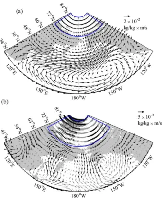
To examine the atmospheric circulation associated with an increase of moisture flux, we estimated the mean horizontal moisture fluxes in JAS for 1979–2014 and their difference before and after 2002 (2002–14 minus 1979–2001), respectively (Fig. 6). It is notable that the anomalous circulation pattern transports the enhanced moisture from the North Pacific over Russia and into the APS, west of;1608E. The northward moisture flux to the east of the date line over Alaska is reduced for the same period. It seems that the increased moisture flux into the APS is not only due to the increased specific humidity from the North Pacific Ocean but also due to the increased poleward velocity in this sector.
FIG. 4. Difference of mean latent heat flux during JAS before and after 2002 (2002–14 minus 1979–2001). Negative means enhanced heat release from ocean. Black dots denote regions where the dif- ference is statistically significant at the 90% confidence level.
FIG. 5. (a) Zonally averaged (1808–1808) meridional moisture fluxes for 1979–2001 (blue) and 2002–14 (red) and their difference (green; 2002–14 minus 1979–2001) during JAS. Gray shadings in- dicate the mean differences are statistically significant different at the 90% confidence level. (b) As in (a), but for the zonal range (110E8–1108W). (c) As in (a), but for the zonal range (1308E–1808).
Next, we investigate how the increased moisture flux from the North Pacific affects the SIA in the APS.
Figure 7a displays the time series of the anomalous JAS-averaged moisture flux into the APS crossing the southern boundary at 708N. A significant difference before and after 2002 is noticeable; the daily mois- ture flux increases 38% from 2.49 3 1023kg kg21 in 1979–2001 to 3.43 31023kg kg21in 2002–14, which is statistically significant at the 90% confidence level.
Concurrently, the increase in specific humidity in the APS is evident from 2002 onward (Fig. 7b). The differ- ence of MF70 before and after 2002 is quantitatively consistent with the increase of the specific humidity in ASO after 2002 (0.1531023kg kg21). Note that MF70 is divided by the area of APS so that its units are iden- tical to that of the specific humidity.
How did the increased lower-tropospheric humidity from 2002 onward result in acceleration of sea ice melting and thus reduction of SIA in the APS? We consider the air–sea energy flux components that could have caused the reduction of SIA in the APS. Among them, downward longwave radiation increased signifi- cantly at the 99% confidence level since 2002 (Fig. 7c).
Concurrently, the cloud liquid water content in the APS also increased rapidly after 2002 and remained at a higher value compared to that before 2002 (Fig. 7d). The correlation coefficients between the MF70 (Fig. 7a) and the specific humidity in the APS (Fig. 7b), cloud water content (Fig. 7d), and the downward longwave radiation are 0.38, 0.43, and 0.22, respectively, with statistical significance at the 95% confidence level except for the downward longwave radiation. The correlations are substantially decreased and insignificant after removing the linear trends, which implies the correlations are primarily due to long-term changes and the contribution from the interannual variability is insignificant. The correlation between MF70 (Fig. 7a) and downward longwave radiation in the APS (Fig. 7c) increases up to 0.34 (96% confidence level) if the width of MF70 is confined to the west of the date line. This coincides with the result that moisture flux anomalies are more prom- inent in the western and central Pacific as we can see in Fig. 5candFig. 6b.
The downward longwave radiation is highly corre- lated with the specific humidity (r5 0.92 at zero lag) because higher humidity increases the greenhouse ef- fect and therefore there is more downward longwave radiation. The mean APS specific humidity increased by 10% from 1.48 3 1023kg kg21 in 1979–2001 to 1.6331023kg kg21in 2002–14. The average difference in downward longwave radiation between the two pe- riods is about 10 W m22, which can melt 0.453106km2 of sea ice with 1-m thickness in a month considering the total area of APS (5.231012m2) and latent heat of ice melting (302 3 106J m23). The mean cloud water content for 2002–14 (0.8531025kg kg21) is about 22%
higher than that for 1979–2001 (0.7031025kg kg21).
These results indicate that moisture originating from the North Pacific affects the cloud water content as well as the specific humidity in the APS and thereby the downward longwave radiation.
It is also found that the upward longwave radiation was enhanced since 2002 and is highly correlated with the downward longwave radiation (r 5 20.96; 99%
confidence level). This indicates that the increase of downward longwave radiation due to the increased specific humidity could also be partially explained as a positive feedback to SIA loss, which would lead to en- hanced upward longwave radiation and increased spe- cific humidity due to surface warming. Therefore, the net longwave radiation (downward minus upward) in- cludes positive anomalies after 2001 (Fig. 7f).
Downward longwave radiation has often been con- sidered as the main factor controlling recent sea ice melting (Francis and Hunter 2006;Kapsch et al. 2013).
Our results suggest that the increased moisture transport
FIG. 6. (a) Mean horizontal moisture flux in the atmosphere during JAS for 1979–2001. (b) The difference before and after 2002 (2002–14 minus 1979–2001). The blue shapes denote the domain of the APS. Black arrows indicate the mean differences are statisti- cally significantly different at the 90% confidence level. Note that the domain and plotting intervals are different for each panel.
from the North Pacific since 2002 primarily drove the increase of downward longwave radiation, which then caused the significant decline of SIA in the APS during that time. It should be noted that downward shortwave radiation is not a main factor accelerating the sea ice melting after 2002 because it is positively correlated
with the SIA variation instead, as the downward short- wave radiation shows a tendency to decrease after 2000 (Fig. 7g). The slight decline in shortwave radiation, on the other hand, appears to be caused by the increase of low-level cloud water content. The other air–sea energy flux components (i.e., latent and sensible heat fluxes) did
FIG. 7. Time series of (a) anomalies of moisture flux into the APS crossing the southern boundary at 708N, (b) APS specific humidity, (c) APS downward longwave radiation, (d) APS cloud liquid water content, (e) APS upward longwave radiation, (f) APS net longwave radiation, (g) APS downward shortwave radiation, (h) APS latent heat flux, and (i) APS sensible heat flux for 1979–2014. All variables are spatially averaged over the APS (708– 858N, 1108E–1108W) and temporally averaged for ASO except (a), which is for JAS. The MF70, specific humidity, and cloud water content are vertically averaged from 1000 to 500 hPa. Red lines in each panel denote the average anomalies for the two periods, before and after 2002. The number indicates the mean value for 1979–2014. Asterisks indicate statistical significance of mean differences between two periods, 1979–2001 and 2002–14. Note that positive values of all the radiative and turbulent heat fluxes represent downward fluxes into the ocean.
not experience a similar rapid change around 2002 (Figs. 7h,i). Note that positive values of all the radiative and turbulent heat fluxes represent downward fluxes into the ocean.
It is noteworthy that the latent heat flux from the ocean to the atmosphere in the APS steadily decreased from the early 1990s to the mid-2000s (i.e., the positive trend inFig. 7has the mean latent heat flux is negative), followed by an increase until 2002. The increased latent heat flux from the ocean to the atmosphere after 2009 may be due to the enhanced local air–sea exchange after the sea ice cover dramatically decreased. This indicates that the increase of specific humidity in the APS around 2002 is largely due to the enhanced lateral moisture transport from the North Pacific rather than the mois- ture flux from the ocean into the atmosphere in the APS, which is increased from the mid-2000s (Fig. 7h).
Figure 8displays the relationship between the changes in the sea ice melting and the associated atmospheric variables in the APS before and after 2002 for each month from April to November. According to previous studies (Kapsch et al. 2013,2014), positive downward longwave radiation anomalies in March and April can control the summer/autumn sea ice by affecting the timing of the onset of the melting season. We also find that the moisture flux convergence and downward long- wave radiation are increased after 2002 in April and May in addition to summer, which is an additional contributor to reduced summer SIA after 2002 by affecting the onset of sea ice melting. The increase of the moisture flux conver- gence into the APS peaks in July–August. This is followed
by the peak increase of the specific humidity in August along with the enhanced downward longwave radiation, which continues to increase during ASO, and leads to a large reduction of sea ice with a delay. Note that the in- crease of the lateral moisture flux convergence in July is 3.1931024kg kg21, which is comparable to the increase of the specific humidity of 2.4331024kg kg21averaged over the APS in August.
The increased total precipitation and evaporation in October (Fig. 8) likely results from a large reduction of sea ice, which subsequently causes a further increase of downward longwave radiation through November. That is, the increased evaporation in the Arctic Ocean due to the sea ice loss results in a further increase of specific humidity in mid-to-late fall, thus acting as a positive feedback to the accelerated sea ice melting initiated by the increased moisture flux from the North Pacific in July–August. Reduction of sea ice cover in fall is shown to result in increased low-level clouds (e.g., Kay and Gettelman 2009;Wu and Lee 2012). Because clouds and air temperature increased by sea ice melting may also influence the downward longwave radiation, the peak of downward longwave radiation exists after the maximum sea ice loss. The low-level clouds could also be the cause of the reduction in shortwave radiation in recent years (Fig. 7g). However, the importance of ice-albedo feed- back cannot be neglected, which is able to increase the net shortwave radiation when the sea ice extent de- creases. In spite of a reduction of incoming downward shortwave radiation, the net shortwave radiation is in- creased since 2007 (not shown), and, concurrently, the net longwave radiation is decreased (Fig. 7f), which is indicative of the importance of ice-albedo feedback following a significant sea ice loss in the early 2000s.
Numerical experiments and satellite observation have also shown similar lagged atmospheric responses to sea ice loss (Kay and Gettelman 2009;Deser et al. 2010).
c. Evidence in a long-term simulation of KCM and reanalysis dataset
Given the short data record, we further investigate the relationship between Arctic SIA and the moisture flux from the North Pacific using a multicentury climate simulation of KCM as well as ERA-20C.Figure 9shows the time series of observed (1979–2014) and modeled SIA (Fig. 9a) and their anomalies (Fig. 9b) in the APS.
The modeled SIA is similar to observations near the start of the data record prior to the recent decline in sea ice (Fig. 9a), supporting a reasonable representation of the sea ice climate by the model. Note that the model does not reproduce the declining trend of SIA by cli- mate warming, as the model is forced with preindustrial greenhouse gas concentrations.
FIG. 8. Mean differences (2002–14 minus 1979–2001) for each month of APS SIA and the associated atmospheric variables for the APS including specific humidity, lateral moisture flux convergence for 1000–500 hPa, downward longwave radiation (DL), total pre- cipitation at the sea surface (TP), and evaporation (EV) at the sea surface. The MF is the integrated moisture flux crossing all boundaries of the APS domain. All values except the SIA are normalized by their max values (Q: 2.43431024kg kg21; MF:
3.19331024kg kg21; DL: 16.188 W m22; TP: 5.60331023mm h21; and EV: 6.45731023mm h21). Filled and unfilled circles indicate that the increase or decrease is statistically significant above the 90%
and 75% confidence level, respectively.
To make a fair comparison between the KCM and observations, we removed the linear trend from the latter to remove the global warming signal (Fig. 9b). The amplitude of the SIA variations in the model is;0.43 106km2, about half of that in observations. The spec- trum of modeled SIA shows significant peaks on various time scales, ranging from interannual to multidecadal (Fig. 9c). A strong peak exists at periods of about 20–
30 years, indicating a strong multidecadal variation in the SIA.Swart et al. (2015)found decadal and multidecadal internal variability in September Arctic sea ice extent by examining trends in observations, 102 realizations from 31 models in phase 5 of the Coupled Model In- tercomparison Project (CMIP5), and 30 realizations from the Community Earth System Model, version 1, Large Ensemble. They showed that 7- and 14-yr trends of sea ice extent were primarily driven by interrealization spread (i.e., internal variability).Kay et al. (2011)argued that the internal variability explained approximately half of the observed 1979–2005 Arctic sea ice extent loss in September. Therefore, the reproduced decadal internal variability of the SIA in the APS is in accordance with that in other climate models.
Next, we analyze the relationship between the mois- ture flux and SIA in the KCM to support the findings based on observations. The time series and lead–lag correlations of the SIA, MF70, and specific humidity in the APS in June–August (JJA) are shown inFig. 10. All
time series are low-pass filtered with a cutoff period of 10 yr to coincide with the cutoff length in the regime shift test of the observed SIA. And as a statistically significant spectral peak exists around the 20–30-yr pe- riod in the modeled SIA (Fig. 9c), we choose the cutoff period of 10 years to focus on an interdecadal variation (;20-yr period) of the moisture flux from the Pacific. A negative correlation between MF70 and SIA indicates the sea ice melting in the APS is correlated with the increase of moisture flux from the North Pacific (Fig. 10a). The maximum correlation is about 20.4, which is statistically significant at the 95% confidence level. The specific humidity in the APS shows a positive correlation with MF70, which supports the findings that the moisture flux from the North Pacific is responsible for the increased specific humidity in the APS (Fig. 10b).
We note that the lead–lag correlation suggests the in- creased MF70 slightly leads the increase of specific hu- midity in the APS.
While the climate model results are consistent with the satellite-era observational analysis record that star- ted in 1979, the latter only contained one regime shift in 2002. To further verify whether the KCM results for the relation between the MF70 and the SIA are consistent with the available longer observations, we analyze long- term reanalysis data that extend from 1900 to 2010. The MF70 is calculated following the methodology used in the present study. Linear trends of the MF70 and the
FIG. 9. Time series of (a) total SIA in the APS and (b) anomalies after removing a linear trend from the ob- servations (HadISST1; blue) and a control simulation with the KCM (black). (c) Power spectrum of the SIA in the APS from the KCM control simulation.
SIA are also removed. Note that all the time series are low-pass filtered with a cutoff period of 10 years to co- incide with the cutoff length in the regime shift test of the observed SIA.
Figure 11shows the time series and lead–lag correla- tions of SIA and MF70 in ASO when the correlations are maximum and statistically significant. The lines are low-pass-filtered time series with a cutoff period of 10 years. The MF70 has a negative correlation with SIA in the APS, which is consistent with our results from the climate model. The correlation is about20.5, which is statistically significant at the 95% confidence level. We
note that the modeled MF70 is calculated with monthly mean values of specific humidity and meridional veloc- ity components, while MF70 in observations is estimated with 6-hourly data of the same components.
To examine if the variation of lateral moisture flux is related to the warming of the North Pacific, we regress the North Pacific SST on the low-pass-filtered MF70 for 1900–2010 (Fig. 12). The regressed SST field exhibits a negative PDO-like pattern, which is similar to the pat- terns in Fig. 3. The MF70 is statistically significantly correlated with the warming of the western and central North Pacific at the 90% confidence level. The
FIG. 10. (a) Time series and lead–lag correlation of MF70 and SIA in the APS during JJA from the KCM simulation. (b) As in (a), but for the MF70 and the domain-averaged specific humidity in the APS. Blue and red symbols indicate statically significant correlation at the 90% and 95% confidence level, respectively. The statistical significance was estimated by a block bootstrap method dividing the filtered data into 50 blocks of 10-yr length.
FIG. 11. Time series and lead–lag correlation of the SIA (black bars with the 10-yr low-pass-filtered curve shown as blue line) and the MF70 (orange line) during ASO. Blue and red symbols indicate statically significant corre- lation at the 90% and 95% confidence level, respectively. The statistical significance was estimated by a block bootstrap method dividing the filtered data into 11 blocks of 10-yr length.
regression pattern suggests that the SST variation of the western and central North Pacific can affect the SIA in the APS through increased lateral transport of the spe- cific humidity to the Arctic.
4. Summary and discussion
A statistically significant regime shift in sea ice area (SIA) occurred in the Arctic Pacific sector (APS) around 2002; the SIA during ASO has decreased substantially in the last few decades and its declining trend became steeper since the early 2000s. Based on the results from the satellite-era observations and reanalysis in addition to a climate model simulation, we suggested that the warming of the western and central North Pacific con- tributed to the accelerated SIA decrease since the early 2000s. A key mechanism appears to be the enhanced poleward moisture transport from the North Pacific to the Arctic Ocean. Subsequently, specific humidity in the APS significantly increased along with an increase of downward longwave radiation beginning in 2002, which accelerated the decline of SIA of this sector. A multi- centennial climate simulation also showed a negative (positive) correlation between the moisture transport from the Pacific and the SIA (specific humidity) in APS, supporting the observational finding that the enhanced moisture transport from the Pacific led to the increased humidity and then sea ice melting in the APS.
In addition to moisture transport, other factors may also influence Arctic sea ice. First, the low-frequency variability in ocean heat transport from the North Pacific to the Arctic can also be considered to explain the cor- relation of the Pacific SST and the APS SIA (Shimada et al. 2006;Zhang 2015). In particular, there is a trend toward increasing heat transport through the Bering Strait (Woodgate et al. 2012). However, it is unclear whether ocean heat transport dramatically changed
around 2002 mainly owing to a lack of long-term data.
Mizobata et al. (2010)showed that the maximum ocean heat flux occurred in 2004 over the period of 1999–2008, and the same magnitude of heat flux was estimated from 2005 to 2007. The heat transport through the Bering Strait appears to be more strongly correlated with the local Arctic atmospheric circulation, including the summer Arctic dipole that has high interannual variability (Wang et al. 2009). Nevertheless, the effect of heat transport by ocean currents could precondition the acceleration of sea ice melting in the 2000s through gradually thinning the sea ice over a longer period of time.
Second, a change in the local Arctic atmospheric cir- culation, which is not explicitly considered in this study, can also reduce sea ice area in the APS. For example, the negative Arctic dipole, which corresponds to a positive mean sea level pressure (MSLP) anomaly in the Beaufort Sea region and a negative MSLP anomaly on the Siberian side of the Arctic, can enhance the sea ice export through the Fram Strait (Tsukernik et al. 2010;Overland et al.
2012). However, the Arctic dipole primarily shows large interannual variability without a persistent negative phase except during 2007–12 (Overland et al. 2012).
Lindsay and Zhang (2005)suggest a negative PDO re- duces the strength of the anticyclonic Beaufort Gyre and increases the rate of advection of thick ice out of the east Siberian Sea. However, the Arctic Ocean Oscillation Index, which is a measure of the intensity and sense of the wind-driven upper-oceanic circulation in the Arctic Ocean, has stayed in the strong anticyclonic circulation regime since 1997, which does not favor sea ice export through the Fram Strait (Proshutinsky et al. 2015).
It is interesting that the regressed North Pacific SST anomalies are similar to the negative phase of PDO, which may imply a link between the Pacific and the Arctic Ocean (Screen and Francis 2016). The PDO ap- pears to be influenced by several processes including those driven by the atmosphere (Newman et al. 2016).
Regardless of the origin of PDO, the warmer North Pacific Ocean may provide additional moisture into the atmosphere, which then can be transported into the Arctic. The present work suggests a possibility that the change in the North Pacific Ocean toward a negative phase of PDO, which is a warming in the western and central North Pacific, might be associated with the sea ice melting in the APS from 2002. The relationships between the PDO and sea ice reduction should be ex- plored in greater detail in process-based studies.
Acknowledgments. This work was supported by the National Research Foundation of Korea Grant NRF-2009- C1AAA001-0093, funded by the Korean government (MEST), to HJL, YHK, and MOK. S-WY is supported by
FIG. 12. Regression (1038C kg21kg21) of ASO SST on the ASO MF70 for 1900–2010s. Both the MF70 and SST fields are low-pass filtered with a cutoff period of 10 yr. Black dots denote regions where the regression coefficients are statistically significant at the 90% confidence level. The statistical significance was estimated by a block bootstrap method dividing the filtered data into 11 blocks of 10-yr length.
the Korea Meteorological Administration Research and Development Program under Grant KMIPA2015- 1042. Y-OK is supported by the U.S. Department of Energy (DE-SC0014433) and National Science Foun- dation (OCE-1242989). WP acknowledges support from the BMBF project CLIMPRE InterDec (FKZ:
01LP1609B).
REFERENCES
Comiso, J. C., C. L. Parkinson, R. Gersten, and L. Stock, 2008:
Accelerated decline in the Arctic sea ice cover.Geophys. Res.
Lett.,35, L01703, doi:10.1029/2007GL031972.
Dee, D. P., and Coauthors, 2011: The ERA-Interim reanalysis:
Configuration and performance of the data assimilation system.
Quart. J. Roy. Meteor. Soc.,137, 553–597, doi:10.1002/qj.828.
Deser, C., R. Tomas, M. Alexander, and D. Lawrence, 2010: The seasonal atmosphere response to projected Arctic sea ice loss in the late twenty-first century. J. Climate, 23, 333–351, doi:10.1175/2009JCLI3053.1.
——, ——, and L. Sun, 2015: The role of ocean–atmosphere coupling in the zonal-mean atmospheric response to Arctic sea ice loss.
J. Climate,28, 2168–2186, doi:10.1175/JCLI-D-14-00325.1.
Francis, J. A., and E. Hunter, 2006: New insight into the dis- appearing Arctic sea ice.Eos, Trans. Amer. Geophys. Union, 87, 509–511, doi:10.1029/2006EO460001.
——, and S. J. Vavrus, 2012: Evidence linking Arctic amplification to extreme weather in mid-latitudes.Geophys. Res. Lett.,39, L06801, doi:10.1029/2012GL051000.
Gimbert, F., D. Marsan, J. Weiss, N. C. Jourdain, and B. Barnier, 2012: Sea ice inertial oscillations in the Arctic Basin.Cryo- sphere,6, 1187–1201, doi:10.5194/tc-6-1187-2012.
Graversen, R. G., T. Mauritsen, M. Tjernström, E. Källén, and G. Svensson, 2008: Vertical structure of recent Arctic warm- ing.Nature,451, 53–56, doi:10.1038/nature06502.
——, ——, S. Drijfhout, M. Tjernström, and S. Mårtensson, 2011:
Warm winds from the Pacific caused extensive Arctic sea-ice melt in summer 2007. Climate Dyn., 36, 2103–2112, doi:10.1007/
s00382-010-0809-z.
Honda, M., J. Inoue, and S. Yamane, 2009: Influence of low Arctic sea-ice minima on anomalously cold Eurasian winters.Geo- phys. Res. Lett.,36, L08707, doi:10.1029/2008GL037079.
Hopsch, S., J. Cohen, and K. Dethloff, 2012: Analysis of a link between fall Arctic sea ice concentration and atmospheric patterns in the following winter.Tellus,64A, 18624, doi:10.3402/
tellusa.v64i0.18624.
Jaiser, R., K. Dethloff, D. Handorf, A. Rinke, and J. Cohen, 2012:
Impact of sea ice cover changes on the Northern Hemisphere atmospheric winter circulation.Tellus,64A, 11595, doi:10.3402/
tellusa.v64i0.11595.
Kapsch, M. L., R. G. Graversen, and M. Tjernström, 2013:
Springtime atmospheric energy transport and the control of Arctic summer sea-ice extent.Nat. Climate Change,3, 744–
748, doi:10.1038/nclimate1884.
——, ——, T. Economou, and M. Tjernstrom, 2014: The impor- tance of spring atmospheric conditions for prediction of the Arctic summer sea ice extent.Geophys. Res. Lett.,41, 5288–
5296, doi:10.1002/2014GL060826.
Kay, J. E., and A. Gettelman, 2009: Cloud influence on and re- sponse to seasonal Arctic sea ice loss.J. Geophys. Res.,114, D18204, doi:10.1029/2009JD011773.
——, M. M. Holland, and A. Jahn, 2011: Inter-annual to multi- decadal Arctic sea ice extent trends in a warming world.
Geophys. Res. Lett.,38, L15708, doi:10.1029/2011GL048008.
Kim, B.-M., S.-W. Son, S.-K. Min, J.-H. Jeong, S.-J. Kim, X. Zhang, T. Shim, and J.-H. Yoon, 2014: Weakening of the stratospheric polar vortex by Arctic sea-ice loss.Nat. Commun.,5, 4646, doi:10.1038/NCOMMS5646.
Kug, J.-S., J.-H. Jeong, Y.-S. Jang, B.-M. Kim, C. K. Folland, S.-K.
Min, and S.-W. Son, 2015: Two distinct influences of Arctic warming on cold winters over North America and East Asia.
Nat. Geosci.,8, 759–762, doi:10.1038/ngeo2517.
Lee, S., S. B. Feldstein, D. Pollard, and T. S. White, 2011a: Do planetary wave dynamics explain equable climates?J. Climate, 24, 2391–2404, doi:10.1175/2011JCLI3825.1.
——, T. Gong, N. Johnson, S. B. Feldstein, and D. Pollard, 2011b:
On the possible link between tropical convection and the Northern Hemisphere Arctic surface air temperature change between 1958 and 2001.J. Climate,24, 4350–4367, doi:10.1175/
2011JCLI4003.1.
Lindsay, R. W., and J. Zhang, 2005: The thinning of Arctic sea ice, 1988–2003: Have we passed a tipping point?J. Climate,18, 4879–4894, doi:10.1175/JCLI3587.1.
Madec, G., 2008: NEMO ocean engine. L’Institut Pierre-Simon Laplace Note du Pole de Mod^ élisation 27, 193 pp.
Maslanik, J., J. Stroeve, C. Fowler, and W. Emery, 2011: Distri- bution and trends in Arctic sea ice age through spring 2011.
Geophys. Res. Lett.,38, L13502, doi:10.1029/2011GL047735.
Mizobata, K., K. Shimada, R. Woodgate, S.-I. Saitoh, and J. Wang, 2010: Estimation of heat flux through the eastern Bering Strait.
J. Oceanogr.,66, 405–424, doi:10.1007/s10872-010-0035-7.
Newman, M., and Coauthors, 2016: The Pacific decadal oscil- lation, revisited. J. Climate, 29, 4399–4427, doi:10.1175/
JCLI-D-15-0508.1.
Overland, J. E., and M. Wang, 2010: Large-scale atmospheric cir- culation changes are associated with the recent loss of Arctic sea ice.Tellus,62A, 1–9, doi:10.1111/j.1600-0870.2009.00421.x.
——, J. A. Francis, E. Hanna, and M. Wang, 2012: The recent shift in early summer Arctic atmospheric circulation.Geophys. Res.
Lett.,39, L19804, doi:10.1029/2012GL053268.
Park, W., N. Keenlyside, M. Latif, A. Ströh, R. Redler, E. Roeckner, and G. Madec, 2009: Tropical Pacific climate and its response to global warming in the Kiel climate model.J. Climate,22, 71–92, doi:10.1175/2008JCLI2261.1.
Proshutinsky, A., D. Dukhovskoy, M.-L. Timmermans, R. Krishfield, and J. L. Bamber, 2015: Arctic circulation regimes.Philos. Trans.
Roy. Soc. London,373A, 20140160, doi:10.1098/rsta.2014.0160.
Rayner, N. A., D. E. Parker, E. B. Horton, C. K. Folland, L. V.
Alexander, D. P. Rowell, E. C. Kent, and A. Kaplan, 2003:
Global analyses of sea surface temperature, sea ice, and night marine air temperature since the late nineteenth century.
J. Geophys. Res.,108, 4407–4435, doi:10.1029/2002JD002670.
Rodionov, S. N., 2004: A sequential algorithm for testing climate regime shifts. Geophys. Res. Lett., 31, L09204, doi:10.1029/
2004GL019448.
Roeckner, E., and Coauthors, 2003: The atmospheric general cir- culation model ECHAM5. Part I: Model description. Max Planck Institute for Meteorology Rep. 349, 127 pp.
Screen, J. A., and I. Simmonds, 2010: The central role of dimin- ishing sea ice in recent Arctic temperature amplification.
Nature,464, 1334–1337, doi:10.1038/nature09051.
——, and J. A. Francis, 2016: Contribution of sea-ice loss to Arctic amplification is regulated by Pacific Ocean decadal variability.
Nat. Climate Change,6, 856–860, doi:101038/nclimate3011.
——, C. Deser, and I. Simmonds, 2012: Local remote controls on observed Arctic warming.Geophys. Res. Lett., 39, L10709, doi:10.1029/2012GL051598.
Serreze, M. C., M. M. Holland, and J. Stroeve, 2007: Perspectives on the Arctic’s shrinking sea-ice cover.Science,315, 1533–
1536, doi:10.1126/science.1139426.
Shimada, K., T. Kamoshida, M. Itoh, S. Nishino, E. Carmack, F. McLaughlin, S. Zimmermann, and A. Proshutinsky, 2006:
Pacific Ocean inflow: Influence on catastrophic reduction of sea ice cover in the Arctic Ocean.Geophys. Res. Lett.,33, L08605, doi:10.1029/2005GL025624.
Strang, G., 1986:Introduction to Applied Mathematics. Wellesley- Cambridge Press, 758 pp.
Stroeve, J. C., M. C. Serreze, M. M. Holland, J. E. Kay, J. Malanik, and A. P. Barrett, 2012: The Arctic’s rapidly shrinking sea ice cover: A research synthesis.Climatic Change,110, 1005–1027, doi:10.1007/s10584-011-0101-1.
Strong, C., G. G. Magnusdottir, and H. Stern, 2009: Observed feedback between winter sea ice and the North Atlantic Oscil- lation.J. Climate,22, 6021–6032, doi:10.1175/2009JCLI3100.1.
Swart, N. C., J. C. Fyfe, E. Hawkins, J. E. Kay, and A. Jahn, 2015:
Influence of internal variability on Arctic sea-ice trends.Nat.
Climate Change,5, 86–89, doi:10.1038/nclimate2483.
Tsukernik, M., C. Deser, M. Alexander, and R. Tomas, 2010:
Atmospheric forcing of Fram Strait sea ice export: A closer look. Climate Dyn., 35, 1349–1360, doi:10.1007/
s00382-009-0647-z.
Valcke, S., 2013: The OASIS3 coupler: A European climate modelling community software.Geosci. Model Dev.,6, 373–
388, doi:10.5194/gmd-6-373-2013.
Vihma, T., 2014: Effects of Arctic sea ice decline on weather and climate: A review.Surv. Geophys.,35, 1175–1214, doi:10.1007/
s10712-014-9284-0.
Von Storch, H., and F. W. Zwiers, 1999: Statistical Analysis in Climate Research. Cambridge University Press, 494 pp.
Wang, J., J. Zhang, E. Watanabe, M. Ikeda, K. Mizobata, J. E.
Walsh, X. Bai, and B. Wu, 2009: Is the dipole anomaly a major driver to record lows in Arctic summer sea ice extent?Geo- phys. Res. Lett.,36, L05706, doi:10.1029/2008GL036706.
Woodgate, R. A., T. J. Weingartner, and R. Lindsay, 2010: The 2007 Bering Strait oceanic heat flux and anomalous Arctic sea-ice re- treat.Geophys. Res. Lett.,37, L01602, doi:10.1029/2009GL041621.
——, ——, and ——, 2012: Observed increases in Bering Strait oceanic fluxes from the Pacific to the Arctic from 2001 to 2011 and their impacts on the Arctic Ocean water column.Geo- phys. Res. Lett.,39, L24603, doi:10.1029/2012GL054092.
Wu, D. L., and N. J. Lee, 2012: Arctic low cloud changes as ob- served by MISR and CALIOP: Implication for the enhanced autumnal warming and sea ice loss. J. Geophys. Res.,117, D07107, doi:10.1029/2011JD017050.
Zhang, J., R. Lindsay, M. Steele, and A. Schweiger, 2008:
What drove the dramatic retreat of Arctic sea ice during summer 2007?Geophys. Res. Lett.,35, L11505, doi:10.1029/
2008GL034005.
——, ——, A. Schweiger, and M. Steele, 2013: The impact of an intense summer cyclone on 2012 Arctic sea ice retreat.Geo- phys. Res. Lett.,40, 720–726, doi:10.1002/grl.50190.
Zhang, R., 2015: Mechanisms for low-frequency variability of summer Arctic sea ice extent.Proc. Natl. Acad. Sci. USA,112, 4570–4575, doi:10.1073/pnas.1422296112.