Anomalous Heat Transport in Low-Dimensional Quantum Spin Systems

(1)

Anomalous Heat Transport in

Low-Dimensional Quantum Spin Systems

Inaugural-Dissertation

zur

Erlangung des Doktorgrades

der Mathematisch-Naturwissenschaftlichen Fakult¨ at der Universit¨ at zu K¨ oln

vorgelegt von

Michael Hofmann

aus Bretten (Baden)

K¨oln 2002

(2)

Berichterstatter: Prof. Dr. A. Freimuth Priv.-Doz. Dr. G.S. Uhrig

Vorsitzender der Pr¨ ufungskommission: Prof. Dr. L. Bohat´ y

Tag der m¨ undlichen Pr¨ ufung: 07. Januar 2002

(3)

Introduction

Low-dimensional systems show unusual, rich, and fascinating physical properties. A well- known example for the peculiar physics in one dimension, predicted by Peierls already in 1955, is the Peierls instability of one-dimensional metals. This instability leads to a metal- insulator transition with an insulating so-called charge density wave (CDW) groundstate, consisting of a periodic charge density modulation accompanied by a periodic lattice distor- tion. Another possible groundstate is the spin density wave (SDW) state. In one-dimensional antiferromagnets an analogous instability, the so-called spin-Peierls transition, may occur with a non-magnetic groundstate of singlet pairs and an energy gap for spin excitations.

An important aspect of the physics in low dimensions is the presence of quantum-ﬂuctuations.

For example, a one-dimensional Heisenberg antiferromagnet does not show magnetic ordering even at zero temperature; both, the groundstate and the excitation spectrum are determined by strong quantum fluctuations. Another example is the physics of one-dimensional metals with electron-electron interactions. It is believed that these systems cannot be described by the usual Fermi liquid picture involving well defined quasiparticle excitations, common to the description of conventional metals and semiconductors. Instead, more exotic scenarios like the Tomonaga-Luttinger liquid are believed to be appropriate with fascinating properties, as for example, spin/charge separation, where independent spin and charge excitations with dif- ferent velocities are formed. In two dimensions the influence of strong quantum fluctuations is also of much current interest and strongly debated, since it is directly related to the physics of the high-temperature superconductors, which are obtained by doping a two-dimensional Heisenberg antiferromagnet with mobile charge carriers.

A fresh impetus to the field of low-dimensional systems has been given by the discovery of a variety of materials in the last few years, in which such low-dimensional structures are real- ized. For example, a number of cuprates and vanadates with low-dimensional spin structures – spin chains, spin-ladders, as well as various planar spin arrangements – are now available as good single crystals. Also, various one-dimensional conductors are known, most notably the organic conductors and among those the so-called Bechgaard salts. These systems are, to some researchers, the most interesting and fascinating materials ever discovered. Their physics displays the complete set of unusual phenomena typical for low-dimensional materi- als, including unconventional superconductivity, spin/charge separation, spin-Peierls, CDW-, and SDW-transitions as well as a plethora of effects driven by magnetic fields like a field

1

(6)

2

CHAPTER 1. INTRODUCTION

induced spin density wave state with quantized Hall-resistance.

The groundstate, the excitation spectrum as well as various thermodynamic properties, such as the speciﬁc heat and the magnetic susceptibility of many low-dimensional spin systems have been studied quite intensively in the last few years. In contrast, much less is known about the dynamics of magnetic excitations, e.g., the microscopic understanding of how they transport energy, and their coupling to the lattice degrees of freedom. Nevertheless, such studies appear to be quite promising, as, for example, magnetic excitations are expected to move without dissipation in a spin 1/2 Heisenberg chain with nearest neighbor coupling.

A valuable tool for the study of the dynamics of magnetic excitations and of their cou- pling to the lattice is provided by measurements of the thermal conductivity as a function of temperature, magnetic field and doping. The challenge of this thesis was therefore a sys- tematic experimental study of the thermal conductivity of low-dimensional spin systems in a wide range of temperature, magnetic field and in various materials with different magnetic properties. Our results are indeed very remarkable and promising: First, a sizeable magnetic contribution to the heat current may occur in systems with large magnetic coupling and it may even dominate the total thermal conductivity at rather high temperatures of a few hundred Kelvin. To our knowledge these cases provide the first class of insulators, in which the domi- nant mechanism of heat transport at high temperatures is non-phononic. Second, the phonon heat current is strongly influenced by the presence of magnetic excitations, as signaled, e.g., by a strong damping and by a magnetic field dependence of the phononic thermal conductivity.

The course of this thesis is the following: In chapter 2 an introduction to low-dimensional systems is given. The basic ideas of heat transport in solids are sketched out in chapter 3. A detailed description of the experimental setup and of the calibration procedure, necessary to conduct high resolution heat transport measurements is given in chapter 4.

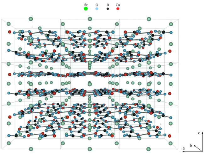
Chapter 5 deals with the thermal conductivity of the 2-d spin liquid system SrCu

₂

(BO

₃

)

₂

. Among the 2-d spin 1/2 systems SrCu

₂

(BO

₃

)

₂

is an intriguing compound with fascinating physical properties. The spin structure realizes the Shastry-Sutherland model which was studied theoretically 20 years ago. One ﬁnds a spin dimer ground state with extremely local- ized magnetic excitations. Furthermore, quantized magnetization plateaus can be observed in striking contrast to classical spin systems where the magnetization increases monotonically.

The heat transport parallel and perpendicular to the 2-d spin system is studied and compared to analytical results. It turns out that the interplay between phonons and magnetic excita- tions plays a central role for the heat transport. We will suggest a consistent interpretation of the thermal conductivity data in terms of resonant scattering of phonons by magnetic ex- citations, worked out with the collaboration of G.S. Uhrig.

Chapter 6 is devoted to the quasi 1-d spin-Peierls system CuGeO

₃

. Before the discovery

of CuGeO

₃

all known systems exhibiting a spin-Peierls transition were organic compounds,

e.g., (TMTTF)

₂

PF

₆

. The discovery of CuGeO

₃

, the ﬁrst inorganic spin-Peierls compound,

has renewed the interest in studying this phenomenon as large crystals of high quality have

been synthesized allowing, e.g., precise neutron scattering experiments. A systematic study

of the thermal conductivity as a function of temperature and as a function of the magnetic

ﬁeld along all three crystallographic directions is presented for pure CuGeO

₃

. Anomalous

(7)

3 temperature dependence of the thermal conductivity along two crystallographic directions is found. In addition, κ depends strongly on the applied magnetic ﬁeld. A discussion of the ex- perimental results, including numerical calculations of possible magnetic contributions to the heat current and anisotropy considerations, is presented subsequently. Thermal conductiv- ity data of Zn and Mg doped CuGeO

₃

accomplish the experimental investigations on CuGeO

₃

. In chapter 7 a systematic study of the heat transport as a function of temperature and of the magnetic field in the Bechgaard salts is presented. To our knowledge, these measure- ments provide the first systematic study of heat transport in these materials at high and low temperatures. We find an anomalous magnetic field and temperature dependence of κ, irrespective of whether the systems are metallic or insulating. We will see that the Luttinger liquid picture and in particular the scenario of spin/charge separation, discussed for these materials, may be an appropriate picture for an understanding of the findings. A detailed discussion and model calculations for the heat transport complete this chapter.

Chapter 8 deals brieﬂy with the heat transport in Sr

₂

CuO

₂

Cl

₂

. This compound is isostructural

to La

₂

CuO

₄

, the parent compound of the high-temperature superconductors. The thermal

conductivity of La

₂

CuO

₄

is known to be anomalous, but its interpretation is still under de-

bate [1]. This stems from lattice instabilities making diﬀerent thermal conductivity scenarios

possible. Sr

₂

CuO

₂

Cl

₂

is free from these complications which facilitates the interpretation of

the thermal conductivity results. A discussion of our ﬁndings and a comparision to the previ-

ously obtained thermal conductivity data of La

₂

CuO

₄

and of YBa

₂

Cu

₃

O

₆

are presented [1,2].

(8)

4

CHAPTER 1. INTRODUCTION

(9)

Chapter 2

The Physics of Low-Dimensional Systems

Over several decades low-dimensional systems have attracted considerable interest since they are well-suited to investigate the properties of strongly interacting electron systems with a variety of possible groundstates. Besides charge density wave (CDW) or spin density wave (SDW) groundstates, superconductivity can also be observed. Thus it is argued that low- dimensional model systems help towards a better understanding of the superconducting state.

As the ﬁeld is relatively large, I will focus my attention on the instabilities and particular- ities in quasi-one-dimensional systems. I start from low-dimensional conductors discussing the Peierls-transition, the CDW groundstate and SDW transition. Finally, the spin-Peierls transition will be presented.

2.1 Quasi-One-Dimensional Conductors

Loosely speaking, low-dimensional conductors are materials with strongly anisotropic electri- cal conductivity. Hence, for a perfectly one-dimensional conductor we would expect a ﬁnite electrical conductivity along one direction and no electronic transport along the other two directions. The highly anisotropic electronic transport is closely related to the anisotropic nature of the crystal structure. Atoms form linear chains where the orbitals strongly overlap.

This is for example seen in the so-called perylene radical cation salts (e.g. (PE)

₂

PF

₆

× 2/3 THF), where the building blocks are planar molecules arranged in such a way that a strong overlap of the orbitals occurs only perpendicular to these planes [3, 4]. In the molecule planes the overlap between the orbitals are much weaker or possibly zero. Hence, for certain electron conﬁgurations a one-dimensional conduction band along the chain direction is formed where the delocalization of the electrons results in a relatively large electrical conductivity along the chains. Perpendicular to the chains the electrons are localized and little or none electrical conductivity is expected.

However, in nature there are no perfect one-dimensional conductors. The conducting chains are embedded in a three-dimensional lattice and very often the interchain overlap cannot be completely neglected. Thus we speak of quasi-one-dimensional conductors.

5

(10)

6

CHAPTER 2. THE PHYSICS OF LOW-DIMENSIONAL SYSTEMS

0 1

q

Two dimensions One dimension

q = 2k_F q = 2k

F

kF

-k_F

0 k

0

k_y

kx

T = 0K

3d 2d 1d

χ(q)/χ(0)

2k_F

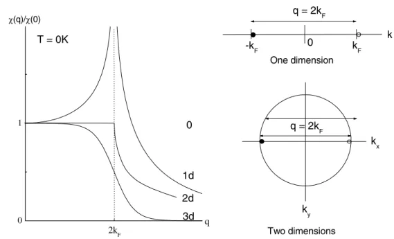
Figure 2.1: Left: Polarisation function χ(q) for the one-, two- and three-dimensional case at T = 0. Right: Fermi surface in one (1-d) and two dimensions. According to Kagoshima et al. [5].

2.1.1 Peierls Instability and the CDW Groundstate

A salient feature of quasi-one-dimensional metals is the Peierls transition in conjunction with an insulating ground state [5]. This so called charge density wave (CDW) ground state is a consequence of the properties of the density response function χ(q) of a one-dimensional electron gas

χ(q) ∝ 1 q ln

q + 2k

_F

q − 2k

F

. (2.1)

Fig. 2.2 shows χ(q) for a one-, two- and three-dimensional free electron gas [5]. In one dimen- sion a logarithmic divergency occurs, while for the other two dimensions χ(q) remains ﬁnite.

The diﬀerent response functions arise from the diﬀerent dimensionality of the Fermi surfaces.

The right panel of Fig. 2.2 shows the Fermi surfaces of an ideal one- and two-dimensional Fermi surface. In one dimension the Fermi surface consists of two points at ± k

_F

. In the two dimensional case the surface is a circle.

Let us now discuss what this means for the electron system. The Pauli exclusion principle

states that electrons can be scattered into empty states only. As the energies of the phonons

are very small ( k

B

T ) compared to the energies of the electrons, only electrons in the

vicinity of the Fermi surface can participate in scattering processes. For a one-dimensional

Fermi surface there are thus two processes to consider. First, the scattering of electrons by

phonons with wave vectors q ≈ 0, i.e., energy and momentum of the electrons are approxi-

mately conserved. Second, processes where phonons with wave vectors q ≈ 2k

_F

are absorbed

or emitted, changing the wavevector of the electrons from k ≈ ± k

_F

to k ≈ ∓ k

_F

, i.e., the

electrons are scattered from one side of the Fermi surface to the other (see Fig. 2.1). Thus if

a phonon wants to change the electron momentum it must have the wavevector 2k

_F

. In other

words, one phonon mode (2k

_F

) interacts virtually with all electrons for which the scattering

is allowed. In the one-dimensional case χ(q) diverges at q = 2k

F

. This is sometimes called

(11)

2.1. QUASI-ONE-DIMENSIONAL CONDUCTORS

7

x a

a)

ρ(x)

k

-π/a -k_F k_F _π/a

E_F

0 E_k

2a x

b)

k

-π/a -k_F k_F π/a

E_F

0 E_k

2∆

ρ(x)

Figure 2.2: Peierls transition illustrated on the basis of a one-dimensional model. The half-ﬁlled conduction band and the electron density ρ(x) are outlined for the undistorted chain (a). The electron density smoothly varies with the lattice periodicity. Insulating CDW ground state (b) with a static lattice distortion. The electron density is modulated with a periodicity of 2k_F. The lattice constant is denoted by a.

“perfect nesting”. The pairs of states, one full and one empty, diﬀering by 2k

F

and having the same energy, give a divergent contribution to χ(q). In higher dimensions the number of such states is strongly reduced, indicated by the upper 2k

_F

wavevector of the 2-d case in Fig. 2.1(left). This leads to the reduction of the singularity of χ(q) at 2k

_F

.

However, Peierls instabilities are not restricted to one-dimensional systems only. If the energy spectrum meets certain conditions the transition occurs also in higher dimensions, e.g., in the layered transition metal oxides NbSe

₂

and TaS

₂

[6].

To illustrate the Peierls transition we start with the simple situation of a one-dimensional metal (Fig. 2.2 a) with equidistant atoms. First, the situation of a half-ﬁlled conduction band is considered. In the nearly free electron approximation, the electron wave functions are the well known Bloch states where the electron density ρ(x) smoothly varies with the lattice periodicity [7]. Let us now shift the atoms from the equilibrium positions according to u = u

₀

· cos(2k

F

x), as illustrated in Fig. 2.2 b). This leads to a doubling of the unit cell. Hence, the reciprocal lattice vector changes from 2π/a to π/a. The border of the ﬁrst Brillouin zone is now at the Fermi wavevector k

_F

. Consequently, an energy gap opens at the Fermi level where all states below the gap are ﬁlled and the states above are empty. The former metal has transformed into a semiconductor with a gap. The electron density ρ(x) is now modulated with a periodicity of 2k

_F

.

Is the CDW state energetically favourable? To answer this, we must consider the balance between the gain of electronic energy δE

_el

(due to the lowering of the occupied states) and the loss of elastic energy δE

dis

, resulting from the distortion of the lattice.

The change of the total energy was calculated by Kagoshima [5]

δE = δE

_el

+ δE

_dis

≈ − ∆

²

χ(q, T ) − κ 2g

²

, (2.2)

(12)

8 where g denotes the electron-phonon coupling constant and κ denotes the elastic constant.

The polarisation function χ(q, T ) diverges with T → 0 and q = 2k

_F

, while the elastic constant is finite. Hence, for finite g the Peierls transition takes place at finite temperature

¹

. The transition temperature follows from δE(T = T

P

) = 0 and is given by

k

_B

T

_P^{M F}

= 1.1E

_F

exp ( − 1/λ

₀

) with λ

₀

= | g

²

D(E

_F

) |

¯

hω

₂_k_F

(2.3)

where λ

₀

the dimensionless electron-phonon coupling constant, ω

₂k_F

the high-temperature phonon frequency leading to the Peierls instability and D(E

_F

) is the density of states at the Fermi level.

Some Theoretical Results

The formation of the CDW and the Peierls transition are two sides of the same coin. To elucidate this one has to take a closer look at the Fr¨ ohlich Hamiltonian in momentum space describing a one-dimensional system consisting of electrons and phonons [8].

H =

k,σ

(k)ˆ c

^†_k,σ

ˆ c

_k,σ

+

q

ω

_q

ˆ b

^†_q

ˆ b

_q

+ 1 2

+

k,σ

q

g(q)ˆ c

^†_k₊_q,σ

ˆ c

_k,σ

ˆ b

^†₋_q

+ ˆ b

_q

(2.4) The ﬁrst term describes the electron system with Bloch eigenstates. The corresponding elec- tron energies are measured with respect to the chemical potential. The second term represents the phonon energy, where the simplest case with only one acoustical phonon branch is con- sidered. Finally, the electron-phonon interaction is given by the last term with the coupling constant g(q) [8]. This expression can be interpreted in terms of scattering electrons from a state | k > to a state | k ± q > by absorbing/emitting a phonon with wavevector q (-q).

I want to consider the mean field results now [9]. One should keep in mind that fluc- tuation effects which are neglected by the mean field theory are particularly important in one-dimensional systems. Here, they are so strong that no long range order occurs at finite temperatures. However, the always present three-dimensional coupling between the chains in real systems allows the formation of a Peierls phase for temperatures above T = 0. For further reading about fluctuation effects at the Peierls transition, please refer to the following references [10–14].

Subsequently, I will show on a basic level how the CDW state follows from the Fr¨ ohlich Hamiltonian. The transition to the CDW state is related to the “vanishing” of the 2k

_F

phonon mode, i.e., a static lattice distortion occurs for T ≤ T

P

. Thus, the associated mean values < b

_±2_k_F

> are diﬀerent from zero.

In the ﬁrst step one keeps in the interaction term only the terms with q = ± 2k

_F

. Next, the operators ˆ b

_±2k_F

are replaced by their mean values < b

_±2k_F

>:= b. Retaining only these terms we ﬁnd

H =

k,σ

(k)ˆ c

^†_k,σ

ˆ c

k,σ

+

k,σ

g(2k

F

)ˆ c

_k_±2_k† F

ˆ

c

k

· 2b + ω(2k

F

)b

²

. (2.5)

1Note, that according to the Mermin-Wagner theorem, ordering in strictly one-dimensional systems does not take place even for T→0.

(13)

9 From Eq. 2.5 the average energy E =< H > can be obtained and reads

E = E

₀

+ g(2k

_F

)

k,σ

ˆ c

^†_k_±2_k

F,σ

c ˆ

_k

· 2b + ω(2k

_F

)b

²

, (2.6) where E

₀

is the expectation value of the ﬁrst term in Eq. 2.5. A minimization of E with respect to b yields

b = − g ω <

k,σ

ˆ c

_k_±2_k†

F

ˆ

c

_k

> . (2.7)

The righthand side of Eq. 2.7 is not zero as b = 0. Eq. 2.7 can now be related to the average electron density which is given by

ˆ

ρ(x) =

q

ρ

_q

e

^iqx

(2.8)

and its q-th component by the Fourier transform ˆ

ρ

_q

=

k,σ

ˆ

c

^†_k_±_q,σ

ˆ c

_k,σ

. (2.9)

the average number density is therefore equal to the righthand side of Eq. 2.7. In the metallic state only < c ˆ

^†_k

c ˆ

_k

> = 0 ⇒ < ˆ c

^†_k₋_q

c ˆ

_k

>= ρ

₀

δ(q). Thus, together with Eq. 2.8 one gets

< ρ(x) >= ρ

₀

= constant. In the CDW ground state, however, one has in addition <

ˆ c

^†_k₋₂_k

F

c ˆ

_k

>= ρ

₁

δ(q − 2k

_F

). Thus the average density is given by

< ρ(x) >= ρ

₀

+ ρ

₁

e

ⁱ²^k^F^x

(2.10) which implies a modulation of the CDW with a period of 2k

_F

. Eqs. 2.7-2.10 show the close relationship between the distortion of the lattice and the CDW groundstate. The CDW and the lattice distortion with wavevector 2k

F

are proportional to each other and have the same periodicity. It should be noted here that this is also the case for a conventional metal, where the Bloch waves are modulated with the periodicity of the lattice. The crucial diﬀerence is the collective formation of the CDW ground state, where the 2k

F

component of ρ(x) dominates all others.

The results obtained by a much more rigorous treatment on the mean ﬁeld level are summa- rized below [8, 9].

The modulation of the charge density wave reads

ρ(x) = ρ

₀

+ ρ

₁

cos(2k

_F

x + φ) ρ

₁

= ρ

₀

∆

λ

₀

¯ hv

_F

k

_F

, (2.11) where λ

₀

is the dimensionless electron phonon coupling constant, v

_F

the Fermi velocity, k

_F

the Fermi wave vector and φ the phase. The corresponding displacement at site n is given by

u

n

=

2 ω

₂_k_F

∆

g cos(2k

F

na + φ) . (2.12)

Both ρ(x) and u

n

are related to a complex order parameter

∆ = ∆e ˆ

⁽^iφ⁾

(2.13)

(14)

10 describing the phase transition. The energy gap is given by

1 = λ

₀

E_F

0

1

²

+ (∆(T ))

²

tanh

²

+ (∆(T))

²

2k

_B

T

d (2.14)

and

∆(0) = 1.76k

B

T

M F

(2.15)

which is formally equivalent to the temperature dependence of the gap of BCS-superconductors.

For a priori soft phonons a strong renormalisation of the phonon spectrum occurs in the vicinity of 2k

_F

(Kohn anomaly). The new phonon frequencies are

Ω

²_q

= ω

²_q

1 − 2g

²

¯ hω

q

χ(q, T )

≤ ω

_q²

(2.16)

with the unrenormalised phonon frequency ω

_q

[9]. The temperature dependency of the 2k

_F

mode reads

Ω

²₂_k

F

= λ

₀

ω

₂²_k

F

ln(T /T

_P^{M F}

) (2.17)

where λ

₀

and T

_{M F}

denote the electron-phonon coupling constant and the transition temper- ature in mean ﬁeld theory respectively. That is the formation of a static lattice deformation arises with T → T

M F

. Below the transition temperature, the phonon dispersion relation also changes substantially due to the change in the size of the Brillouin zone [5]. This implies that the degenerate phonon branch splits into an optical and an acoustical phonon branch.

It can be shown that these branches correspond to the elementary excitations of the CDW, the so-called A

₋

and A

₊

modes [5]. The A

₊

mode corresponds to a modulation of the am- plitude (amplitudons) of the CDW and the A

₋

to a phase modulation (phasons). While the amplitudons are gapped, the phason modes are gapless excitations which may be regarded as a sliding of the CDW along the chain, requiring no energy for q → 0.

The sliding without resistance is only possible if the CDW is incommensurate to the lattice, i.e., the ratio of the wavelength of the CDW and the periodicity of the lattice is irrational

²

. However, the translation invariance of the Fr¨ ohlich Hamiltonian is broken when the ratio of the wavelength of the CDW and the periodicity of the lattice is rational (commensurable), when impurities in the lattice interact with the CDW or when the CDWs on the 1-d chains interact with each other. In these cases the sliding motion of the CDW is suppressed. One often speaks of this as the “pinning of the CDW”. The sliding charge density waves can con- tribute to the electrical conductivity in a large frequency range [15]. Moreover, the sliding of the CDW is related to extraordinary transport phenomena, e.g., nonlinear conduction, current oscillations and interference eﬀects [16–19].

Experimental Indication of the CDW

The Peierls transition can be identiﬁed by dc-conductivity or X-ray measurements. The CDW can be observed by measuring, e.g., the microwave conductivity. In Fig. 2.3 a measurement

2Actually, the irrationality requirement is too strong, because commensurability eﬀects are only important for ratios of, e.g., 1/2 or 2/3. For “higher” ratios, e.g. 1/4, 1/8, etc., commensurability eﬀects become weaker [5].

(15)

11 0 50 100 150 200 250 300

10

^-5

10

^-4

10

^-3

10

^-2

10

^-1

10

⁰

10

¹

10

²

σ

_||

σ

σ (S/ cm )

Temperature (K)

Figure 2.3: Longitudinal (•) and transversal (◦) microwave conductivity of the perylene radical cation salt (PE)₂PF₆ ×2/3 THF.

along and perpendicular to the highly conducting chains of the quasi-one-dimensional con- ductor (PE)

₂

PF

₆

× 2/3 THF is shown

³

. The system belongs to the so-called perylene radical cation salts. Compared to a conventional metal, the absolute value of σ

_||

is rather low. As the transverse conductivity is three orders of magnitude smaller than σ

_||

, the system is proved to be a quasi-one-dimensional conductor. The low absolute value of σ is attributed to domain walls hampering the electrical conductivity.

The Peierls transition takes place at around 118 K resulting in an activated behavior of the conductivity. Note that the conductivity drops by about four orders of magnitude in a rela- tively narrow temperature range.

Due to impurities in the lattice the CDW is pinned and no additional contribution to the dc-conductivity is expected. However, the CDW contribution to σ is frequency dependent (σ(ω) ∝ ne

²

δ(ω − ω

₀

)), where ω

₀

≈ 10 GHz is the resonance frequency of the CDW. This results in an enhancement of σ(ω) [4]. The local maximum in σ at 30 K is an indication of charge density waves as a similar eﬀect is not detected in the dc-conductivity [4].

The temperature dependence of σ

_||

above the transition reﬂects the strong inﬂuence of struc- tural phase transitions on the electrical conductivity. At 151 K the stack molecules rotate and the anions are shifted out of their original positions, indicated by a step in σ

_||

. It is believed that the system becomes higher dimensional which partly suppresses the lattice ﬂuctuations.

This results in a reduction of the electron scattering and therefore in an increase of σ

_||

below 151 K.

3The measurements were conducted in a 10.2 GHz resonant cavity during my diploma thesis at II. Physikalis- ches Institut of the University of Karlsruhe [3].

(16)

12 At 213 K a splitting in two kinds of domains, where the stack molecules are turned into diﬀerent directions, takes place. This leads to additional electron scattering and therefore to a decrease of σ

_||

towards lower temperatures. The transverse electrical conductivity strongly resembles σ

_||

. However, the step in σ

_⊥

at 151 K is smaller that that found in σ

_||

and the splitting of the crystal into two domains at 213 K is almost not visible.

2.1.2 The SDW Transition

The electron-electron interaction can have drastic consequences on the ground state of a one- dimensional metal. The simplest possible Hamiltonian describing such an interaction is given by

H = t

<i,j>,σ

ˆ

c

^†_i,σ

c ˆ

_j,σ

+ U

i

ˆ

n

_i,_↑

n ˆ

_i,_↓

(2.18)

where ˆ n

_i,σ

= ˆ c

^†_i,σ

c ˆ

_j,σ

[19]. This is the so-called Hubbard model, given here in coordinate space. The ﬁrst term describes the kinetic energy of the electrons and the second stands for on-site Coulomb interaction. No electron-phonon interaction is taken into account. The radical limitation to short range interaction is rather severe but the model has proven to be a powerful tool in understanding magnetism and metal-insulator transitions [20].

The spin density wave ground state is thought to arise from electron-electron interaction.

This was shown by Overhauser through a mean ﬁeld approach [21]. As in the case of the CDW state, a gap opens up at the Fermi level and a metal-insulator transition occurs. But in contrast to the CDW state, no lattice distortion takes place. This can be clariﬁed by viewing the SDW as a superposition of two charge density waves – one for the “spin up” and one for the “spin down” subbands which are shifted against each other by φ = π resulting in a cancellation of the charge density modulations, as sketched in Fig. 2.4. The spatial spin modulation is given by

< S >= 2S cos(2k

F

x + φ) (2.19) where S is the amplitude and φ is the phase of the spin density modulation. Spin rotational and translation symmetries are broken in the SDW state. The reason why the symmetry breaks is the gain in energy by pushing the occupied states down while raising the empty states.

λ=π/k_F ρ(x)

ρ(x)

Figure 2.4: Charge and spin density modulation for the two spin subbands in the spin density ground state

As a lattice distortion is absent, the SDW state cannot be observed by structural experiments

(e.g., X-ray ). However, the transition can be observed by, e.g., measuring the electrical con-

ductivity (see chapter 7) or by applying nuclear magnetic resonance and muon spin rotation

techniques [22].

(17)

2.2. ONE-DIMENSIONAL ANTIFERROMAGNETS

13 2.2 One-Dimensional Antiferromagnets

The insulating compound CuGeO

₃

, intensively studied in this thesis, belongs to the class of so-called quasi-one-dimensional antiferromagnets where the magnetic coupling is strongly direction dependent. For quasi-one-dimensional spin-1/2 systems with Heisenberg or XY- magnetic exchange, which also exhibit a large magneto-elastic coupling, the spin-Peierls tran- sition is proposed. This transition is driven by the spin system. A spontaneous breaking of the translation symmetry of the spin system leading to a dimerized ground state causes a gain in magnetic energy. While the spin chains are coupled to the lattice, the singlet formation is tied to a lattice distortion, leading to a loss in elastic energy that has to be overcompensated by the magnetic energy gain to force the transition.

In order to see how the spin-phonon coupling comes into play one may consider the following Hamiltonian

H =

i

J(i, i + 1)ˆ s

i

s ˆ

i+1

+

q,j

¯

hω

₀

(q, j)

ˆ b

^†_q_,j

ˆ b

_q_,j

+ 1 2

. (2.20)

The phonons described by noninteracting bosons are given by the second term where q and j denote the wavenumber and the phonon branch, respectively. A detailed discussion about the spin-Peierls active phonon modes is given by Braden et al. [23]. The interaction between the phonons and the spin system stems from the inﬂuence of a local lattice displacement on the electronic transition matrix elements and hence on the magnetic exchange. To introduce the spin-phonon coupling, J is expanded into a power series of the lattice displacement u(i).

One obtains

J (i, i + 1) = J +

i

(u(i) − u(i + 1)) · ∇

i

J (i, i + 1) + . . . . (2.21) For small phonon displacements it is suﬃcient to retain the linear term of the expansion only.

The spin-Peierls transition is closely related to the Peierls transition of quasi-one-dimensional metals. As discussed in section 2.1.1, metals with half ﬁlling are featured by an instability tending towards dimerisation. It can be shown that for the XY-model the spin operators can be mapped via a Jordan-Wigner-Transformation onto the model of noninteracting spin- less fermions (pseudo fermion representation), i.e., one obtains for the pseudo fermions the bandstructure of a Peierls metal [24]. Thus the spin-Peierls transition can be discussed in the same framework as the Peierls transition. The ground state of the spin-Peierls system is a nonmagnetic singlet state separated by an energy gap ∆ from the excited triplet states.

A brief overview of the theoretical results will be given now. I want to point out that approx- imations concerning, e.g., the phonon system and the so-called four-fermion-terms resulting from the Jordan-Wigner-Transformation are necessary in order to obtain the following rela- tions. For further reading on this subject, there are numerous references [24–31].

The transition temperature in the weak coupling regime (T J) is given by T

_SP

= 0.83pJ exp

− 1 pλ

with λ = 4˜ g

²

ω

²₀

πJ , (2.22)

where ˜ g = ˜ g(2k

_F

) is the linearized spin-phonon coupling constant and ω

₀

= ω

₀

(2k

_F

) the

unrenormalized frequency of the spin-Peierls active phonon mode. The renormalisation con-

stant p resulting from a Hartree-Fock approximation of the four-fermion-terms is within the

(18)

14 E

k

-

_π

/2c

0 _π

/2c

k

-

_π

/c

0 _π

/c

E

J

₁

J

₁

J

₂

J

₂

J

₁

J J

J J J

Figure 2.5: Schematic representation of the excitation spectra for the uniform (left) and dimerized (right) antiferromagnetic Heisenberg chain. The long-dashed curve represents the magnon dispersion. The continuum is found between the two solid lines.

weak coupling limit 1.64. As for Peierls systems, a BCS-like energy gap is predicted with

∆(T = 0) = 1.765 k

_B

T

_SP

. The dimerisation δ in the D-phase leads to a magnetic energy gain of E

_m

∝ δ

²

ln δ [29] and is related to the energy gap via

J

₁_,₂

= J (1 ± δ(T )) and δ(T ) = ∆(T )

pJ . (2.23)

Cross and Fisher succeeded in calculating the transition temperature without the Hartree- Fock approximation of the four-fermion-terms. They obtained

T

_SP

J = 0.8 4˜ g

²

ω

²₀

πJ or T

_SP

= 1.02 g ˜

²

ω

₀²

(2.24)

and in addition, the energy gap ∆ and the magnetic energy gain E

_m

at T = 0 K

∆ ∝ δ

²^/³

and E

_m

∝ δ

⁴^/³

. (2.25)

From Eq. 2.24 it is evident that T

_SP

does not explicitly depend on the coupling constant J , but is merely given by the ratio of the spin-phonon coupling constant ˜ g and the unrenormalized phonon frequency ω

₀

. According to this result the spin-Peierls transition is governed by the lattice properties. A soft lattice and/or a strong spin-phonon coupling favor the spin-Peierls transition.

The schematic representation of the energy spectrum of a one-dimensional antiferromagnetic Heisenberg chain is given in Fig. 2.5. The left panel represents the characteristic features of the uniform chain. For T > T

_SP

one ﬁnds a so-called spinon continuum bound by the upper and lower curves. This continuum results from two S=1/2 excitations, referred to as spinons.

Each spinon is described by the dispersion relation E(k) = π/2J sin(kc), (0 ≤ k ≤ π/c).

(19)

15 Energy and momentum of the two-spinon continuum are given by E(q) = E(k

₁

) + E(k

₂

) and q = k

₁

+ k

₂

, respectively. The lower boundary is found for k

₁

= 0 and k

₂

= q (or vice versa) and the upper boundary for k

₁

= k

₂

= q/2. The peculiar spectrum is related to the degener- acy of the ground state at k = 0, ± π/c where quantum ﬂuctuations lead to an occupation of the states at ± π/c. Because of the gapless excitations the susceptibility remains ﬁnite.

The right panel of Fig. 2.5 shows the main features of the excitation spectrum of the Peierls- distorted one-dimensional spin chain. The non-degenerate singlet groundstate is separated by an energy gap from the triplet (magnon) states for T < T

_SP

, illustrated by the dashed line. The two solid lines enclose the 2-triplet continuum with minimum energy

⁴

of 2∆. The dashed line corresponds to bound states of two spinons.

2.2.1 The Spin-Peierls Systems in Magnetic Fields

The inﬂuence of the magnetic ﬁeld on spin-Peierls systems is taken into account by adding a Zeeman term to Eq. 2.20 which reads:

H

m

= − gµ

B

H

i

s

^z_i

(g 2) . (2.26)

While the non-degenerate singlet groundstate in the D-phase remains unchanged, the ﬁrst excited triplet state splits up resulting in a smaller energy gap ∆ between the singlet ground- state and the ﬁrst excited triplet state.

The singlet groundstate is energetically favorable until the applied magnetic ﬁeld H exceeds a critical value H

crit

. Interestingly, H

crit

is smaller than H = k

B

∆/gµ

B

at T = 0, something one would actually expect. This can be understood by adopting the pseudo fermion picture.

The magnetic field can be seen as a measure of the band filling; or in other words, the Fermi wave vector depends on the magnetic field [32]. In the U-phase the band is half-filled for a zero magnetic field (2k

F

(H = 0) = π/c). A finite magnetic field corresponds to a more than half-filled band. Hence, in finite magnetic fields the realisation of a filled and empty band can only be achieved for an incommensurate (I) lattice distortion. This means that the ratio between the wavevector 2k

F

(H) and π/c is an irrational number. However, for small ﬁelds the transition to the D-phase is stabilized by Umklapp scattering processes while in higher ﬁelds the I-phase is energetically favored.

In the language of the pseudo fermion picture, the deviation from half ﬁlling in the U-phase is given by

₂^∆_π/c^k

which can be calculated via

∆k(H)

2π/c = k

_F

(H) π/c − 1

2 = M gµ

B

= χH gµ

B

, (2.27)

where M is the magnetization of the spin chain given by M = gµ

_B

N

l=1

s

^z_l

. (2.28)

χ denotes the susceptibility, g and µ

_B

are the g-value and the Bohr magneton, respectively.

4Binding eﬀects are neglected here.

(20)

16

0 1 2 3

0.00 0.01 0.02 0.03

0.0 0.5 1.0

0 1 2 3

∆

q

∆

k

g_µ

BH / k

BT

SP(0)

Wavevector ∆q and ∆k (2π/a)

D I

U

gµBH / kBTSP(0)

T_SP(H) / T_SP(0)

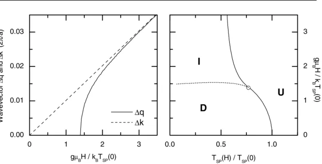
Figure 2.6: Left: Deviation ∆q = q(H)−π/c of the wavevector of the I-phase from that of the D-phase. The diﬀerence between the wavevector favored by the magnetic ﬁeld from π/c is denoted by ∆k = 2k_F(H)−π/c [32]. Right: Universal phase diagram of a spin-Peierls system.

The solid line denotes the calculated phase boundary [32]. The D-I phase boundary is indicated by the dashed line.

The competition between the wavevector q = 2k

F

(H) favored by the magnetic ﬁeld and the wavevector q = 2k

_F

(0) = π/c described by the dimerisation is visualized in Fig. 2.6. Here

∆k(H) = 2k

_F

(H) − π/c and ∆q(H) = q(H) − π/c are plotted. The former describes the deviation from half filling and the latter shows the difference between the wavevector of the distorted lattice of the I-phase and that of the D-phase. In the D-phase substantial differences between 2k

_F

(H) and q = 2k

_F

(0) = π/c are present. Exceeding a critical magnetic ﬁeld, the transition to the I-phase takes place and 2k

F

(H) and q(H) rapidly approach each other with further increasing the ﬁeld.

The right panel of Fig. 2.6 visualizes the universal phase diagram of a spin-Peierls system.

The I-U phase boundary was calculated by Cross [32]. The open circle denotes the so-called Lifschitz-point where the three phase boundaries meet. The numerical result for (T

_L

, H

_L

) reads:

T

_L

0.77 T

_SP⁰

and gµ

B

H

_L

1.38 k

B

T

_SP⁰

. (2.29) Clearly, the transition temperature is reduced by a magnetic ﬁeld. The reduction of T

_SP

for small magnetic ﬁelds is quadratic. The D/U-phase boundary is described approximately by

T

_SP

(H) − T

_SP⁰

T

_SP⁰

− 0.09

gµ

_B

H k

_B

T

_SP⁰

₂

for H → 0 . (2.30)

For higher magnetic ﬁelds the I/U-phase-transition temperature is expected to saturate at

T

_I/U

= 0.5T

_SP⁰

because Umklapp scattering processes stabilizing the D-phase, but there is no

contribution of Umklapp processes in the I-phase anymore. In the dimerized phase, Umklapp

processes cause an eﬀective doubling of the spin phonon coupling constant in Eq. 2.24 leading

(21)

17 to a doubling of the transition temperature compared to the saturation temperature in the I-phase.

As mentioned above, the lattice distortions in the I-phase are characterized by a wave vec- tor q = ∆q(H) + π/c where (2π/c)/q(H) denotes the periodicity of the distortion pattern in units of the lattice constant c. In the framework of the Ginzburg-Landau formalism the structural distortion is described by an order parameter Q. While in the dimerized phase the order parameter is given by an alternating structural distortion with a constant dimerization amplitude ( − 1)

ⁿ

Q the incommensurate phase is featured by a modulation of Q with the wave vector ∆q(H). In the simplest case a sinusoidal modulation of the order parameter is considered and reads:

Q

_n

= ( − 1)

ⁿ

Q

₀

· cos(∆qnc

₀

) , (2.31) where c

₀

describes the original lattice constant along the spin chains [24].

One can also imagine the I-phase made of domains which are still dimerized. In this so-called soliton-lattice model the phase of the dimerization amplitude Q

n

alters by π over a correlation length ξ. The modulation is then given by

Q

n

= ( − 1)

ⁿ

Q

₀

k · sn( nc

₀

kξ , k) , (2.32)

where sn(x, k) stands for the elliptical Jacobi-function with modulus k ∈ [0, 1] given by the distance of the domain walls L = πc

₀

/∆q [33, 34]. We see two interesting cases: for k → 1 Eq. 2.32 transforms to tanh(x) describing a single soliton. For k → 0, accounting for the decreasing soliton distance, sn(x, k) goes over to a sinusoidal modulation. Similar to ∆k(H) (see Eq. 2.27) in the uniform phase, ∆q(H) is related to the magnetization M via

∆q

2π/c = M gµ

B

, (2.33)

where 2π/c describes the reciprocal lattice vector of the undistorted spin chain.

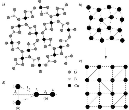
2.2.2 Magnetic Frustration

So far only an antiferromagnetic exchange between the nearest neighbors has been considered.

Taking antiferromagnetic next nearest neighbor interaction into account, frustration comes into play. The one-dimensional spin chain governed by frustration and dimerisation can be described by the Hamilton operator

H =

l

J

1 − ( − 1)

^l

δ

ˆ

s

_l

· s ˆ

_l₊₁

+ J

ˆ s

_l

· s ˆ

_l₊₂

(2.34) where δ accounts for the dimerisation and J

₁_,₂

= J (1 ± δ) stands for the alternating coupling between the nearest neighbors.

In Fig. 2.7 the general phase diagram of dimerized and frustrated spin chains is depicted as

T = 0 [35]. Let us discuss the most important regions. For δ = 0 and J

= 0 one has a

uniform Heisenberg chain that exhibits no gap in the excitation spectrum. For δ = 0 the

groundstate remains gapless as long as the frustration ratio J

/J does not exceed the critical

value α

_c

= 0.2411, obtained by a numerical scaling analysis [36–38]. For J

/J > α

_c

and δ = 0

the groundstate is also dimerized due to spontaneous symmetry breaking, i.e., through the

(22)

18

0.0 0.5

0 1

∆E =0

∆E >0

0.2411 Frustration J'/J

Dimerisation δ Figure 2.7:

Phase diagram of an AFM Heisenberg chain with |S| = 1/2 as function of frustration J/J and dimerisation δ = (J₁ − J₂)/2J at T = 0 [35].

formation of singlet pairs.

Exact results for the groundstate are obtained for the so-called Majumdar-Gosh-point (J

/J =

0.5 and δ = 0) where the groundstate is made up of spin dimers with a ﬁnite energy gap and

for the groundstate on the line 2J

/J + δ = 1, which is a product wavefunction of independent

singlet dimers [39–41]. The system is always gapped as soon as the dimerisation (δ > 0) is

switched on. No analytical results for the groundstate can be obtained in this region.

(23)

Chapter 3

Thermal Transport in Solids

In this chapter a brief and fundamental introduction to the heat transport in solids will be given. This chapter is not intended to be a complete summary of all heat transport mech- anisms known, but is rather concerned with a speciﬁc selection of the basic transport prop- erties of phonons, electrons and magnetic excitations and the interplay between them in an experimentalist’s point of view. Detailed calculations that blur the physics are omitted here.

References will be given concerning the transport properties of “magnons” and the inﬂuence of phonon scattering on magnetic excitations giving an overview of previous experimental and theoretical treatments on magnetic materials.

3.1 Heat Transport by Phonons

A general expression for the thermal conductivity κ on the basis of a kinetic theory has been given by Debye [42]. In the simplest form κ reads

κ = 1

3 cvl , (3.1)

where in the modern language c is the speciﬁc heat of the quasiparticle excitations, v the mean velocity of these particles, and l = vτ the mean free path (τ is the relaxation time).

The theoretical problem of heat transport through an insulating solid has been treated by various research groups [43–47]. The heat transport of phonons is essentially governed by the scattering of phonons on the sample boundary, on lattice imperfections or on defects and phonon-phonon scattering processes. The latter process can be distinguished in normal or so-called N processes which conserve phonon quasi momentum and resistive or so called Umklapp processes. Although N processes do not give rise to thermal resistance they may have a strong impact on other resistive scattering processes as they may alter the occupation of possible phonon states [45, 48, 49].

For a quantitative description of our data, presented in chapters 5 to 8, we will use a Debye model for the phononic thermal conductivity [45–47, 50]. Therefore I want to introduce this central equation here:

κ

^ph

= k

_B

2π

²

v

k

_B

¯ h

₃

T

³

_Θ_D_/T

0

x

⁴

e

^x

τ (ω, T )

(e

^x

− 1)

²

Anomalous Heat Transport in Low-Dimensional Quantum Spin Systems